Dynamic Scheduling Fusion Model for Railway Hazardous Chemical Transportation Emergency Supplies Based on DBSCAN–Bayesian Network

Abstract

Railway hazardous chemical transportation, a high-risk activity that endangers personnel, infrastructure, and ecosystems, directly undermines the sustainability of the transportation system and regional development. Traditional risk management algorithms, which rely on empirical rules, result in sluggish emergency responses (with an average response time of 4.8 h), further exacerbating the environmental and economic losses caused by accidents. The standalone DBSCAN algorithm only supports static spatial clustering (with unoptimized hyperparameters); it lacks probabilistic reasoning capabilities for dynamic scenarios and thus fails to support sustainable resource allocation. To address this gap, this study develops a DBSCAN–Bayesian network fusion model that identifies risk hotspots via static spatial clustering—with ε optimized by the K-distance method and MinPts determined through cross-validation—for targeted prevention; meanwhile, the Bayesian network quantifies the dynamic relationships among “hazardous chemical properties-accident scenarios-material requirements” and integrates real-time transportation and environmental data to form a “risk positioning-demand prediction-intelligent allocation” closed loop. Experimental results show that the fusion algorithm outperforms comparative methods in sustainability-linked dimensions: ① Emergency response time is shortened to 2.3 h (a 52.1% improvement), with a 92% compliance rate in high-risk areas (e.g., water sources), thereby reducing ecological damage. ② The material satisfaction rate reaches 92.3% (a 17.6% improvement), and the neutralizer matching accuracy for corrosive leaks is increased by 26 percentage points, which cuts down resource waste and lowers carbon footprints. ③ The coverage rate of high-risk areas reaches 95.6% (a 16.4% improvement over the standalone DBSCAN algorithm), with a 27.5% reduction in dispatch costs and a drop in resource waste from 38% to 11%. This model achieves a leap from static to dynamic decision-making, providing a data-driven paradigm for the sustainable emergency management of railway hazardous chemicals. Its “spatial clustering + probabilistic reasoning” path holds universal value for risk control in complex systems, further boosting the sustainability of infrastructure.

1. Introduction

Railway transportation, as one of the most important transportation modes globally, undertakes a substantial amount of freight tasks in China, including a large number of hazardous materials transportation operations. In the context of railway transportation, hazardous chemicals are defined as goods with explosive, flammable, toxic, infectious, corrosive, radioactive, or other characteristics that are prone to causing casualties and property damage during transportation, loading/unloading, and storage, thus requiring special protection. Although railway transportation has certain safety advantages in the transportation of hazardous chemicals, it still faces severe safety challenges. Statistical data (as shown in Figure 1: Distribution of railway hazardous chemical transportation accident types) indicate that railway hazardous chemical transportation accidents exhibit multiple typological characteristics. Due to the high-safety risks involved in hazardous chemicals transportation, how to effectively identify risks in the transportation process and reasonably carry out emergency supplies allocation and scheduling has become one of the current research hotspots.

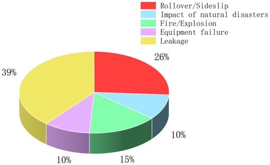
Figure 1. Pie chart of accident type distribution of railway hazardous chemical transportation.

Railway transportation of hazardous chemicals involves flammable, explosive, and corrosive substances. These substances are prone to triggering cascading risks, posing severe threats to public safety, the ecological environment, and the stability of transportation systems.

The cascading effects of such accidents typically exhibit a “chain reaction” characteristic: initial leakage may lead to pipeline corrosion, track deformation, and even derailment of subsequent trains, thereby expanding the scope of disaster impact. This requires emergency management to not only respond to immediate risks but also predict potential secondary hazards—an objective that traditional methods struggle to achieve.

Traditional emergency management relies on empirical rules and suffers from inherent limitations, such as delayed response, insufficient accuracy in risk identification, and poor adaptability between scheduling schemes and dynamic risks.

To address these challenges, this study proposes a fusion model combining the DBSCAN algorithm and Bayesian networks. Specifically, the model identifies high-risk hotspots through density-based clustering (with optimized static parameters ε and MinPts) and quantifies dynamic correlations via probabilistic reasoning (integrating multi-source spatial data). This approach overcomes the limitations of static classification in traditional methods and the defects of independent application of single technologies, enabling closed-loop decision-making from spatiotemporal risk localization to dynamic demand forecasting. Ultimately, it provides a new data-driven paradigm for emergency management in railway hazardous chemical transportation.

2. Literature Review

2.1. Research on Risk Analysis of Railway Dangerous Chemical Transportation

At present, the risk analysis of railway hazardous chemical transportation has developed into a multi-dimensional system encompassing qualitative description and quantitative evaluation. Its core revolves around identifying risk factors, analyzing evolution mechanisms, and innovating evaluation methods. Meanwhile, it has gradually incorporated research insights from cross-disciplinary fields and other transportation modes to refine the risk management framework.

In terms of risk factor identification and qualitative analysis, Gao [1] focused on the inherent physicochemical properties of hazardous chemicals—such as flammability, explosiveness, and toxicity. By establishing a fault tree model, he dissected the weak links in the safety system of railway hazardous chemical transportation, clarifying the fundamental role of fault tree models in the qualitative identification of risk sources. Luan et al. [2] sorted out the causes of accidents from the five dimensions of “human-machine-material-environment-management” based on the principles of safety system engineering. They proposed targeted countermeasures, including the establishment of accident case databases and hazardous chemical property databases, which further improved the classification framework for risk factors. Zhang [3] constructed a comprehensive safety evaluation model using the Fuzzy Analytic Hierarchy Process (FAHP). Through specific case studies; he verified the feasibility of this method in quantifying safety-influencing factors across the five dimensions of “human, machine, material, environment, and management,” supplementing the application scenarios of fuzzy evaluation in risk quantification.

Research on quantitative evaluation and evolution mechanisms presents a trend of multi-method integration. Huang et al. [4] innovatively proposed the “Entropy-TOPSIS-Coupling Coordination Comprehensive Evaluation Method,” dividing the railway hazardous chemical transportation system into five subsystems. The evaluation results showed that the system safety has been gradually improved, yet the human and management subsystems remain weak links—providing a quantitative basis for risk control. Zhang et al. [5] constructed a risk-accident evolution hierarchical network using the Functional Resonance Analysis Method (FRAM). Taking a sodium cyanide leakage accident as an example, they revealed the process by which nonlinear coupling resonance of functional modules leads to accidents, filling the gap in research on the dynamic mechanism of accident evolution. Huang et al. [6] combined the Interpretive Structural Modeling (ISM) with the Bayesian network (BN). Through causal reasoning of 17 risk sub-indicators, they found that “insufficient technical knowledge of transport personnel” exerts the greatest impact on system risk (with a probability of 0.74), offering precise guidance for the control of key risk factors. Zhao et al. [7] verified that “human factors,” “transport vehicle facilities,” and “packaging and loading” are the core factors influencing accidents by leveraging the Bayesian network, combined with Dempster–Shafer evidence theory and the Expectation-Maximization (EM) learning algorithm—further consolidating the critical role of human factors.

Risk analysis methods for other transportation modes also provide valuable references for railway research. Ren et al. [8] constructed a Tree-Augmented Naive Bayes (TAN) model for highway hazardous chemical transportation, analyzing the full-process risks of “pre-accident, in-accident, and post-accident.” They found that human factors tend to cause minor leakage accidents, and rescue time is longer in summer; this “full-process risk assessment” approach can be extended to emergency time planning in railway scenarios. Wang et al. [9] combined Grounded Theory (GT) with BN to quantify the core causal chain of “equipment failure → unsafe tanker state → accident” in highway hazardous chemical transportation, emphasizing the key role of equipment failure and providing a reference for risk control of railway vehicle facilities. In addition, Wu et al. [10] combined BN with Principal Component Analysis (PCA) to evaluate the sustainability of China’s transportation system; their framework of “multi-dimensional indicators + BN quantification” offers cross-disciplinary ideas for the coordinated evaluation of risk and sustainability in railway hazardous chemical transportation. Yusheng et al. [11] assessed the risks of container shipping services based on the PESTLE framework and BN, pointing out that economic and political risks pose the greatest threats; their method of “macro risk classification + BN reasoning” can assist in the analysis of macro-environmental risks in railway hazardous chemical transportation.

2.2. Research on Railway Emergency Material Scheduling Optimization

The optimization of railway emergency material scheduling takes multi-objective modeling as its core and algorithmic innovation as its support, and is gradually moving toward the direction of “dynamic, fair, and precise”. Meanwhile, it incorporates route optimization and cross-domain scheduling logic into the model to enhance the feasibility and adaptability of scheduling schemes.

The development of multi-objective optimization models is the mainstream of the current research. Hu and Li [12] established a multi-objective model with the goals of “maximizing distribution fairness” and “minimizing transportation costs” to address the uncertainties in demand and material shortages post-disaster. By solving the model using an improved genetic algorithm, they verified that the model effectively improves fairness among demand points and reduces costs. Inspired by the concept of hierarchical and zoned prevention and control, Song et al. [13] introduced a fairness indicator of “minimum dissatisfaction degree” and constructed a scheduling model that accounts for disaster severity classification. Using the COVID-19 pandemic in Hubei as a case study, the model achieves a balance between prioritizing severely affected areas and ensuring fairness across all levels, expanding the dimensions of fairness measurement. Zhang et al. [14] focused on the dual objectives of “earliest emergency start time” and “optimal economic efficiency”, establishing a model via multi-objective programming. Case studies confirmed that the model reduces the number of supply points, lowers transportation costs, and enables efficient utilization of materials.

Algorithmic innovation provides technical support for scheduling optimization. To address route optimization for railway hazardous material transportation, Kong et al. [15] introduced adaptability indicators such as “train frequency” and “track gradient”, and constructed a multi-objective 0–1 integer programming model for “safety risk-transportation time-transportation benefit”. Using a hybrid immune–ant colony algorithm to solve the model, they verified that the safety of the route from Jinzhou Station to Jiamusi Station was improved by 84.59%. This “route optimization + multi-objective algorithm” approach provides direct references for the selection of emergency material transportation routes. Yan et al. [16] considered dynamic factors such as road resistance parameters and attenuation coefficients under hazardous weather conditions and built an allocation model that minimizes the sum of “transportation costs + distribution center construction costs + transportation time penalty costs”. Solving the model with the branch-and-bound method, they found that attenuation coefficients and segment disaster intensity play a decisive role in route selection, providing a basis for route optimization in dynamic scenarios.

Scheduling research in other fields also offers new perspectives for railway emergency scheduling. For Kubernetes container scheduling in 5G networks, Farid et al. [17] proposed a classification framework for multi-objective scheduling, categorized as “deterministic-heuristic-learning-based”. Their ideas of “QoS indicator optimization” and “resilience in distributed environments” can assist in the design of objectives such as “material delivery timeliness” and “multi-node collaborative resilience” in railway emergency scheduling. Li et al. [18] proposed the LFRL-MOS dynamic multi-objective framework, which integrates LLM-based fuzzy state fusion, SLA-constrained optimization, and a dual-loop PPO mechanism. This framework optimizes SLA violation rates and response times in medical scheduling scenarios, and its dynamic adjustment logic provides a cross-disciplinary technical reference for emergency scheduling of railway hazardous chemical transportation. Wang et al. [19] constructed a multi-objective logistics routing model based on a graph attention network, enabling real-time scheduling and completing route adjustments within 5 min in dynamic traffic scenarios—this provides technical insights for breaking through the “real-time” bottleneck in scheduling. For international transportation, Zhou et al. [20] proposed a simulation-based Bayesian network (SBN) approach to jointly optimize transportation modes and safety inventory policies. Their concepts of “dynamic lead time estimation” and “multi-decision collaboration” can assist in the joint decision-making of “transportation routes–inventory allocation” for railway emergency materials.

2.3. The Application of Key Technologies in the Transportation and Dispatching of Railway Hazardous Chemicals

As core technologies, the Bayesian network (BN) and the DBSCAN clustering algorithm exhibit significant advantages in addressing uncertainty, dynamics, and data mining. Their application scenarios have expanded from single domains to multi-scenario adaptation, providing substantial support for the technical integration of dynamic scheduling of railway hazardous chemical emergency materials. Leveraging its capability to model uncertainty, the Bayesian network is widely applied in accident risk assessment, handling time estimation, and transportation adaptability evaluation. Chen et al. [21] constructed a BN model for estimating the handling time of hazardous chemical transportation accidents. Through parameter learning using seven nodes (including season, time, and road type) and 902 cases, they achieved probabilistic prediction of three handling time intervals, “0–2 h”, “2–4 h”, and “over 4 h”, and quantified the difficulty ranking of accident handling (rollover > rear-end collision > internal failure, etc.)—providing support for the time prediction of emergency resource allocation. Luan et al. [22] combined the Bow-Tie model with a fuzzy BN to establish a dynamic risk model for hazardous chemical transportation in highway tunnels. By updating accident probabilities through real-time monitoring of node data and simulating the accident impact range using ALOHA software, they realized dynamic risk assessment with “probability-consequence” linkage, and this dynamic update logic can be migrated to railway scenarios. Furthermore, Siyuan et al. [23] applied fuzzy-exact BN to the adaptability evaluation of green shipping services, calculating the safety adaptability of transported objects to address the issue of incomplete BN state coverage. Their idea of “adaptability quantification” can assist in the adaptability evaluation of “materials-demand points” in railway hazardous chemical transportation. The BN studies on highway hazardous chemicals by Ren et al. [8] and Wang et al. [9] (as mentioned earlier) further verify the versatility of BN in multi-scenario risk quantification, laying a foundation for technology migration to railway scenarios. The DBSCAN algorithm demonstrates outstanding performance in data clustering, anomaly detection, and spatial analysis, and is gradually moving toward “parameter self-adaptation” and “multi-scenario adaptation”—providing multiple technical paths for data analysis and scheduling optimization in railway hazardous chemical transportation. In terms of basic scenarios and cross-domain applications, Chen et al. [24] combined DBSCAN with a 3D region-growing algorithm for detecting unstable rock masses on high-angle slopes, achieving rapid clustering of rock mass characteristics and a 71.8% reduction in processing time compared to manual methods. This showcases its advantages in spatial target clustering and provides technical ideas for the spatial division of risk areas along railways. Han et al. [25] introduced DBSCAN into Quality Function Deployment (QFD) to resolve the redundancy issue of numerous Engineering Characteristics (ECs). Through clustering, they accurately identified key ECs, and their ability in data dimensionality reduction and core element extraction can be used for clustering emergency material demand points to improve scheduling efficiency. Shan et al. [26] combined DBSCAN with dynamic K-means++ to realize early identification of voltage inconsistency faults in power batteries (12–23 days earlier than traditional systems). Its anomaly detection capability can be applied to fault early warning of railway hazardous chemical transportation vehicles, providing support for dynamic route adjustment of vehicles in scheduling. Sheng et al. [27] proposed the MSA-iDBSCAN algorithm, which achieves multi-scale ship trajectory clustering through incremental clustering, local refinement, and a quadtree structure—significantly improving clustering efficiency and accuracy. Its features of “multi-scale adaptation” and “efficient query” provide technical potential for multi-region scheduling clustering of railway hazardous chemical transportation routes. To enhance the algorithm’s adaptability, existing studies have optimized DBSCAN parameters and logic: Liang et al. [28] proposed “Descending Neighborhood DBSCAN (DNDBSCAN)” for clustering Physical Machines (PMs) in data centers. Combined with the Cluster Center Nearest (CCN) classification algorithm and the Avoid Hot Spot Time Correlation (AHTC) algorithm, it achieved a balanced utilization rate of PMs of 86% (an 11% improvement compared to comparative algorithms). Its collaborative logic of “clustering-resource allocation” can provide references for resource optimization of emergency material storage nodes. Ng et al. [29] proposed a K-Nearest Neighbors-Probability (KNN-Probability) method for obstacle detection in autonomous driving to dynamically optimize the eps parameter of DBSCAN, and refined clusters based on radial velocity data—achieving a mean Average Precision (mAP) of 0.8942. This idea of “parameter self-adaptation” and “cluster refinement” can solve the problem of “fixed clustering parameters for demand points” in railway emergency material scheduling, improving clustering accuracy. Liu et al. [30] combined adaptive DBSCAN with Stochastic Subspace Identification (SSI) for health monitoring of heritage buildings, resolving issues of dense modes and weak excitation through adaptive parameter selection. Its “parameter self-adaptation” logic can be migrated to “dynamic data clustering” scenarios in railway hazardous chemical transportation (e.g., real-time demand point data). Ma et al. [31] proposed a fast group fusion method for dual-carbon monitoring data based on DBSCAN, realizing efficient data fusion through the calculation of neighborhood distance thresholds and screening of abnormal data. Its “data cleaning-clustering-fusion” process can provide references for the preprocessing of emergency data (e.g., material demand, road conditions) in railway hazardous chemical transportation. Emergency plans for railway hazardous chemical transportation focus on “professionalism, connectivity, and practicality”, with legal compliance and clear definition of responsibilities as the core, to improve the emergency system. Yao and Yang [32], considering the policy environment after the establishment of the Ministry of Emergency Management, proposed three principles for plan formulation: “clarifying the responsibility positioning of enterprises”, “aligning with new legal and regulatory standards”, and “seeking support from government-led professional rescue forces”. Taking the *Emergency Plan for Hazardous Goods Transportation Accidents of China State Railway Group* as an example, they detailed the plan content from aspects such as scope of application, organizational structure, and emergency response—emphasizing the dynamic alignment between the plan and regulations as well as government–enterprise collaboration. This provides a practical framework for the implementation of emergency plans and offers guidance for the role positioning of emergency material scheduling in the plans.

Existing research has made significant progress in risk analysis of railway hazardous chemical transportation, multi-objective scheduling of emergency materials, and application of key technologies, and has fully absorbed experiences from cross-disciplinary fields and other transportation modes. However, there are still three limitations:

First, there is insufficient linkage between risk analysis and scheduling optimization. Most studies conduct risk assessments or scheduling modeling independently, failing to fully integrate dynamic risk information into scheduling decisions. Additionally, there is a lack of targeted adaptation in technology migration from other transportation modes to railway scenarios.

Second, there is a gap in the integrated application of DBSCAN and the Bayesian network. The Bayesian network is mostly used for risk assessment, while DBSCAN is mainly applied to data clustering. The two have not been combined to solve the problem of “spatial clustering and precise scheduling of emergency materials under dynamic risks”, and existing technologies have inadequate parameter adaptability in railway emergency scenarios.

Third, there is insufficient depth of dynamics in scheduling. Existing dynamic scheduling mostly considers single dynamic factors such as road resistance and demand and fails to fully integrate multi-dimensional dynamic information (e.g., accident evolution, rescue time, and material consumption). This makes it difficult to meet the requirements of “real-time response and precise matching” for emergency materials in railway hazardous chemical transportation.

This provides a new idea for data support in the fusion model of this study. The technical roadmap is as follows (Figure 2):

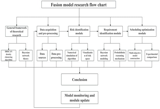
Figure 2. Thought flow chart.

3. Research Methods

3.1. DBSCAN Density Clustering Algorithm

DBSCAN (Density-Based Spatial Clustering of Applications with Noise) is a density-based unsupervised clustering algorithm. Its core idea is to divide density-connected points into the same cluster and identify points in low-density areas as noise points. The algorithm defines density through two key parameters: the neighborhood radius ε and the minimum number of points MinPts.

The theoretical research on the DBSCAN-based emergency supplies allocation model is divided into three stages. First, spatial clustering is carried out based on data, using DBSCAN to identify high-density risk areas in the transportation network. Second, perform parameter setting by defining the neighborhood radius (ε) of the DBSCAN algorithm, which is determined by cross-validation and is usually positively correlated with the average distance between stations; the minimum number of points (MinPts) also needs to be set, which reflects the threshold of regional risk density and needs to be adjusted in combination with historical accident data. Finally, obtain the output results: high-density clusters are key areas where emergency resources need to be prioritized for allocation; noise points are low-risk stations where resource allocation can be simplified. This algorithm can effectively identify density-connected high-risk areas in the transportation network, providing a spatial foundation for subsequent risk assessment and resource scheduling. The clustering process of the DBSCAN algorithm is shown in Figure 3.

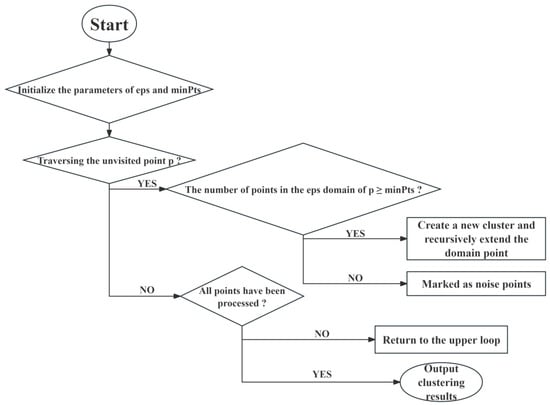
Figure 3. DBSCAN algorithm clustering flow chart.

3.2. Bayesian Network Theory

3.2.1. Fundamentals of Probabilistic Graphical Models

A Bayesian network is a directed acyclic graph (DAG) model based on probabilistic reasoning, composed of nodes and directed edges. Nodes represent random variables, directed edges denote conditional dependencies between variables, and each node is associated with a conditional probability table (CPT) to quantify the degree of dependency. The advantage of Bayesian networks lies in their ability to perform bidirectional inference using prior knowledge and observed data: they can derive results from causes (forward inference) and trace causes from results (backward inference), a feature that grants them unique advantages in uncertainty problems.

3.2.2. Bidirectional Inference Mechanism

① Forward Prediction: Causal inference from risk factors to material demand. For example, if a station is known to belong to a high-risk cluster (Cluster = High) and transports flammable liquids (Hazard Type = Flammable), the inferred probability of a fire (Accident Type = Fire) is 0.65, leading to a 0.85 probability of high material demand (Demand = High).

② Backward Diagnosis: Diagnostic inference from material demand to risk factors. For instance, if high material demand (Demand = High) is monitored in a region, the backward inference gives a 0.73 probability that the accident type is an explosion (Accident Type = Explosion), aiding in locating the accident cause.

3.3. Fusion Model Architecture

The fusion model consists of a risk identification module, a demand prediction module, and a scheduling optimization module. The DBSCAN algorithm divides railway hazardous chemicals transportation stations into risk areas with spatial heterogeneity through density clustering, providing a critical spatial context support for the probabilistic inference of the Bayesian network. This spatial clustering result not only reveals the distribution law of hazardous chemical types in the transportation network but also provides a data foundation for setting prior probabilities in the Bayesian network by quantifying the compositional characteristics of hazardous chemicals in different risk-level areas. As prior knowledge input into the Bayesian network, this spatial distribution feature can significantly improve the probabilistic inference accuracy of hazardous chemical type nodes, thereby optimizing the subsequent prediction logic for accident types and material demands. Meanwhile, the Bayesian network transforms static spatial clustering results into a knowledge system with dynamic decision-making value by constructing a probabilistic transmission chain of “hazardous chemical characteristics-accident scenarios-material demands”. By learning the impact weights of variables such as hazardous chemical transportation volume and environmental factors on accident risks, the network can refine and adjust the risk levels defined by spatial clustering at the probabilistic level based on real-time transportation data. Finally, a multi-objective optimization model with objectives of response time, scheduling cost, and resource waste rate is constructed to solve the optimal scheduling scheme.

4. Data Acquisition and Processing

4.1. Data Source

① Spatial data: Spatial clustering based on the DBSCAN algorithm requires the latitude and longitude coordinates of the site. Based on the real-time map, the following data were obtained, as shown in Table 1.

Table 1. Site latitude and longitude coordinates.

Site Name	Latitude (° N)	Longitude (° E)
Liuzhuang Station	34.123	113.456
Dongming Station	34.789	111.234
Sanmenxia West Railway Station	34.567	113.789
Xiaolizhuang Station	33.869	113.052
Qixian Station	35.291	115.123
Kuofanxian Station	35.321	113.923
Junction Station	34.732	113.611
Baofeng Station	35.851	115.472
Xinzheng Station	35.621	114.201
Tangyin East Railway Station	34.402	113.721
Xinxiang Station	35.912	114.356

② Transportation data: The data of this study are from the dangerous goods transportation management system of the Zhengzhou Railway Bureau, covering the operation records of 11 major hazardous chemical transportation stations within the jurisdiction from 2020 to 2023. The data set contains the total number of vehicles and total tonnage of each station from 2021 to 2023. According to the ‘Dangerous Goods Classification and Name Number’ (GB 12268-2025) [33] standard, the number of sub-items and tons of flammable liquids, flammable solids and corrosive substances were divided, as shown in Table 2 below.

Table 2. Transportation data of each station.

Site Name	Flammable Liquid Tonnage (F)	Tons of Corrosive Substances (C)
Liuzhuang Station	4,410,155	0
Dongming Station	3,730,493	0
Sanmenxia West Railway Station	0	1,650,995
Xiaolizhuang Station	409,264	0
Qixian Station	490,035	0
Kuofanxian Station	212,434	0
Junction Station	62,601	0
Baofeng Station	35,557	0
Xinzheng Station	0	0
Tangyin East Railway Station	0	420
Xinxiang Station	0	229

③ Environmental data: Environmental data around the site (within a 5 km buffer zone), as shown in Table 3.

Table 3. Environmental data of each site.

Site Name	Population Density (Person/km2)	Number of Schools	Number of Hospitals	Water Source Distance (km)	Residential Area (km2)	Industrial Area (km2)
Liuzhuang Station	820	3	2	1.8	12.5	8.3
Dongming Station	650	2	1	2.5	9.2	10.5
Sanmenxia West Railway Station	410	1	1	0.8 (a tributary of yellow river)	5.7	15.3
Xiaolizhuang Station	320	1	0	3.2	4.1	6.8
Qixian Station	210	0	0	4.5	2.3	3.1
Kuofanxian Station	180	0	0	5.1	1.8	2.5
Junction Station	150	0	0	6.2	1.2	1.5
Baofeng Station	120	0	0	7.3	0.8	0.5
Xinzheng Station	100	0	0	8.1	0.5	0.3
Tangyin East Railway Station	90	0	0	9.5	0.3	0.2
Xinxiang Station	85	0	0	10.2	0.2	0.1

④ Material data: Emergency reserve point material data (the latest inventory in 2023), as shown in Table 4.

Table 4. Material data of each site.

Name of Reserve Point	The Site	Fire Fighting Equipment (Box)	Chemical Defense Equipment (Sets)	Medical Supplies (Boxes)	Plugging Material (Tons)	Neutralizer (Tons)	The Maximum Scheduling Amount (Tons)
Zhengzhou Central Repository	Liuzhuang Station	1200	800	1500	30	25	500
Luoyang branch Warehouse	Dongming Station	800	600	1000	20	15	300
Sanmenxia Warehouse	Sanmenxia West Railway Station	600	700	800	25	30	350
Xinxiang Warehouse	Xinxiang Station	300	200	500	10	5	150
Shangqiu Warehouse	Xiaolizhuang Station	400	300	600	15	8	200

4.2. Data Preprocessing Method

The original data had problems such as missing values, outliers, and inconsistent data formats. For numerical missing values, the mean interpolation method was used; for abnormal values, a box plot was used to identify and eliminate data with obvious deviations. At the same time, the latitude and longitude data were standardized by Z-score, using X’ = ${\displaystyle \frac{X-\mu }{\sigma }}$, where is the mean and is the standard deviation, and the dimensional influence is eliminated. Secondly, the risk weight index was constructed. R = ${\displaystyle \frac{1.5F+1.2C}{max(1.5F+1.2C)}}$ represents the normalized risk weight, where F is the transport volume of flammable liquid and C is the transport volume of corrosive substance. The weight settings of 1.5 for flammable liquids and 1.2 for corrosive substances are determined based on national regulatory standards, with specific basis as follows:

① Regulatory standard reference: According to ‘Classification and Risk Assessment of Hazardous Chemicals’ (GB 30000.1-2024) [34], hazardous chemicals are divided into nine categories, and the “hazard degree grade” of each category is specified. Among them, flammable liquids (Category 3) are classified as “high hazard” (hazard grade 2), and corrosive substances (Category 8) are classified as “medium hazard” (hazard grade 3). The standard recommends that the risk weight ratio of high-hazard to medium-hazard substances should be 1.2–1.6:1. The set weights (1.5:1.2) fall within this range, meeting the regulatory requirements for risk quantification.

② Industry standard verification: Refer to ‘Technical Specification for Risk Assessment of Railway Hazardous Goods Transportation’ (TB/T 3550-2022) [35], which stipulates that in the risk index calculation of railway hazardous chemicals transportation, the weight of flammable liquids should be 1.4–1.6, and the weight of corrosive substances should be 1.1–1.3. The weights of 1.5 and 1.2 in this study are the median values of the recommended ranges in the specification, ensuring representativeness and rationality.

The weights of 1.5 and 1.2 meet the national and industry standards, which ensures the scientificity and applicability of the risk weight index under the railway hazardous chemical transportation scenario. Finally, the classification data is coded and converted to ensure that the data is complete, and the format is unified, which lays the foundation for cluster analysis.

5. Construction and Implementation of Fusion Model

5.1. Risk Identification Module

DBSCAN cluster analysis was carried out on the allocation of emergency materials for hazardous chemical transportation in the Zhengzhou Railway Bureau. The optimal parameters were determined through a two-step static optimization:

Optimization of ε (neighborhood radius): ε was determined by visual analysis of the K-distance diagram (k = 4, referring to the average number of adjacent stations in the study area). The K-distance curve (Figure 4) shows an inflection point at ε = 0.35 (corresponding to the actual distance of about 35 km), where the number of noise points is minimized (only two stations: Xinxiang Station and Tangyin East Station), accounting for 18.2% of total stations—lower than ε = 0.30 (3 noise points) and ε = 0.40 (4 noise points).

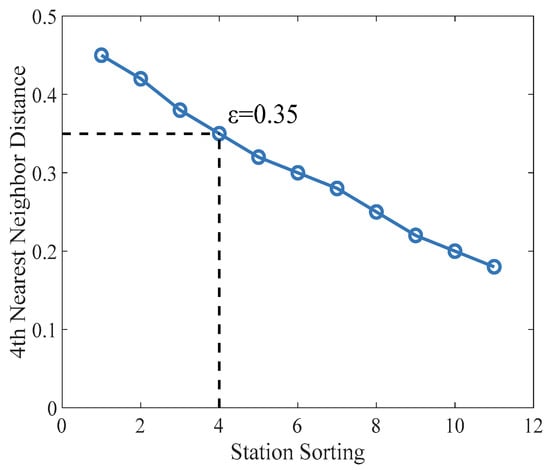
Figure 4. DBSCAN k-distance graph (k = 4).

Calibration of MinPts (minimum number of points): MinPts was evaluated via contour coefficient (a clustering quality index). When MinPts = 4, the contour coefficient reaches 0.72 (>0.7), indicating excellent clustering separation; when MinPts increases to 5 or 6, the contour coefficient decreases to 0.65 and 0.61, respectively (Figure 5), and the clustering effect deteriorates. Therefore, MinPts = 4 is determined as the optimal parameter.

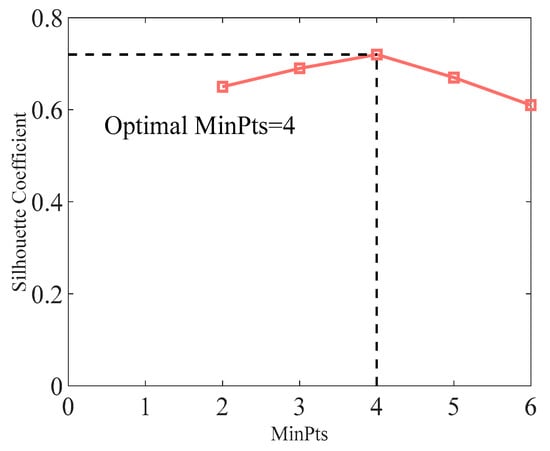
Figure 5. DBSCAN silhouette coefficient vs. MinPts.

In the results of the DBSCAN clustering, different colors represent different clustering labels, and the algorithm divides each station into several clusters according to the geographical location of the station. Each cluster represents a geographically relatively concentrated station group. In the spatial distribution of noise points, DBSCAN labels stations with density lower than MinPts = 4 as noise. There are no other stations within 50 km around Xinxiang Station, and the business volume is very low, so it is impossible to form clusters. Although Tangyin East Station is adjacent to Qixian Station, the density condition is not satisfied due to the large difference in total tonnage. According to the geographical distribution characteristics, the noise points are mostly located at the edge of Henan Province (such as Xinxiang Station) or at the end of the transportation network (such as Tangyin East Station), as shown in Figure 6.

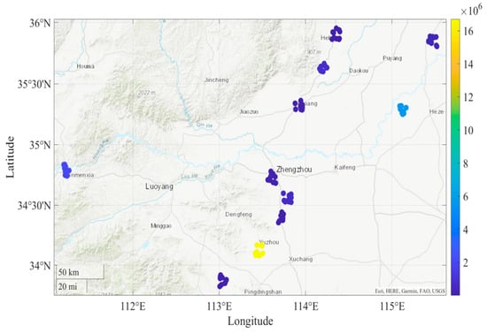
Figure 6. DBSCAN algorithm clustering.

Combined with Figure 7 for analysis. Figure 7 shows the geographical distribution of all stations, their DBSCAN clustering results (C1/C2/C3/noise points), and material volume information, with station locations represented by latitude and longitude. To intuitively distinguish clustering categories (consistent with Table 5: Spatial clustering results), the figure adopts category-based color and shape coding, with specific design rules as follows: high-risk cluster C1 (Liuzhuang Station, Dongming Station), marked with red solid circles (red indicates high risk, solid circles represent core transportation hubs), consistent with the 65.2% transportation volume proportion in Table 5; medium-risk cluster C2 (Sanmenxia West Station, Xiaolizhuang Station), marked with blue hollow circles (blue indicates medium risk, hollow circles distinguish from C1), matching the 28.1% transportation volume proportion in Table 5; low-risk cluster C3 (Qixian Station, Fanxian Station, Junction Station, Baofeng Station, Xinzheng Station), marked with green solid triangles (green indicates low risk, triangles differentiate from circular markers for high/medium risk), corresponding to the 6.7% transportation volume proportion in Table 5; noise points (Tangyin East Station, Xinxiang Station), marked with black crosses (black weakens visual weight, crosses identify non-cluster low-risk stations), in line with the “<1%” transportation volume in Table 5.

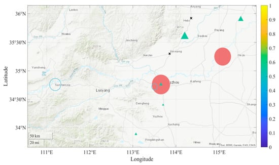
Figure 7. Railway hazardous material transportation station distribution and material volume.

Table 5. Spatial clustering results.

Cluster	Contains Sites	Proportion of Transportation Volume	Risk Level
C1	Liuzhuang Station, Dongming Station	65.2%	High
C2	Sanmenxia West Station, Xiaolizhuang Station	28.1%	Moderation
C3	Qixian Station, Fanxian Station, Jiaojie Station, Xinzheng Station, Baofeng Station	6.7%	Low
Noise pixels	Tangyin East Station and Xinxiang Station	<1%	Very low

By drawing the double vertical axis diagram, the left side is the histogram of the risk index, and the right side is the line chart of the emergency material demand. Compare the risk index and emergency material demand and analyze the relationship between the two, as shown in Figure 8.

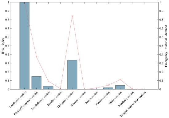
Figure 8. Comparison of risk and emergency material demand at each site.

In addition, spatial dimension analysis is carried out according to the three-dimensional risk spatial distribution. On the vertical axis (risk value), the Z-axis height of Liuzhuang Station is significantly higher than that of other stations, forming a ‘risk peak’, which directly reflects its core position in the transportation of hazardous chemicals. In terms of horizontal distribution, Dongming Station (115.123° E) and Fanxian Station (115.472° E) have similar longitude but large latitude differences, and the Z-axis height is medium, indicating that the risks of the two are derived from different types of dangerous goods. In the low-risk plain area, the Z values of Xinxiang Station and Tangyin East Station are close to the bottom, which is consistent with the conclusion of the heat map. A three-dimensional perspective can assist decision makers in identifying ‘high-risk corridors’, as shown in Figure 9.

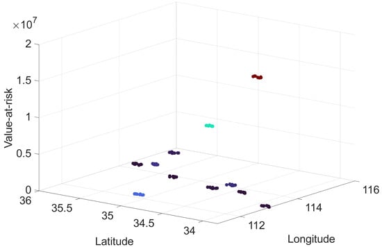
Figure 9. Three-dimensional risk spatial distribution map.

The spatial clustering results show that the DBSCAN algorithm divides 11 sites into three clusters and two noise points, as shown in Table 5.

The high-risk cluster C1 is concentrated in the main line of Longhai Railway, which undertakes more than 60% of the transportation volume of flammable liquid, and the accident frequency is significantly higher than that in other areas. The medium-risk cluster C2 is mainly transported by corrosive substances, which is close to the chemical industry park. The low-risk cluster C3 has a small and scattered traffic volume with noise points, and the accident risk is low.

5.2. Requirement Identification Module

5.2.1. Network Structure Design

The Bayesian network contains five nodes (Table 6), and the edge relationship is determined by expert knowledge and the K2 algorithm—Cluster → HazardType: high-risk clusters are more inclined to transport flammable liquids (P (T1|C1) = 0.92); HazardType → AccidentType: Flammable liquid is easy to cause fire (P (S2|T1) = 0.65), and corrosive substances are easy to cause leakage (P (S1|T2) = 0.78); AccidentType + Environment → Demand: Fire + densely populated areas drive up demand for medical supplies (P (D1|S2, E1) = 0.85).

Table 6. Bayesian network nodes.

Node Name	State Number	Mode Definition
Cluster	3	High risk, medium risk, low risk
HazardType	2	Flammable liquid, corrosive substances
AccidentType	3	Leakage, fire, explosion
Environment	3	Population-intensive areas, industrial areas, suburbs
Demand	3	High demand, medium demand, low demand

Based on the two-way inference mechanism of the Bayesian network mentioned above, (1) Heat map Figure 10 visualizes the conditional probability distribution of hazardous chemical types: the probability of flammable liquids in high-risk clusters is 0.92, which is consistent with the actual transportation data; the probability of corrosive substances in the medium-risk cluster is 0.75, which reflects the transportation characteristics of chemical parks such as Sanmenxia West Station. The probability of two types of hazardous chemicals in the low-risk cluster is close (0.55 vs. 0.45), because the transport category is more complicated. The color shades intuitively show the probability difference, which provides a quantitative basis for the forward reasoning of Bayesian networks (such as pushing Hazard Type from Cluster). (2) Heat map Figure 11 shows the demand probability under different accident–environment combinations: the high demand probability of fire-populated areas is 0.95, due to the surge in demand for evacuation and medical rescue; the high demand probability of leakage in industrial areas is 0.88, which requires a large number of chemical defense equipment and industrial emergency equipment; the probability of explosion in suburban areas with high demand is 0.75, due to the wide range of influence but low population density. The graph supports the reverse diagnosis of Bayesian networks (such as deducing Accident Type from Demand) and provides demand traceability for emergency scheduling.

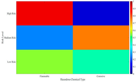
Figure 10. Hazard Type conditional probability table Heat map.

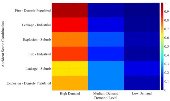
Figure 11. Demand conditional probability table Heat map.

The network structure is constructed by using MATLAB 2023a Bayes Net Toolbox, and the edge weight is determined by data learning. For example, the edge weight from Cluster to Hazard Type is 0.89, which reflects the strong influence of cluster labels on the type of hazardous chemicals. The edge weight from Accident Type to Demand is 0.76, indicating that the type of accident is the main driving factor of material demand, as shown in Figure 12.

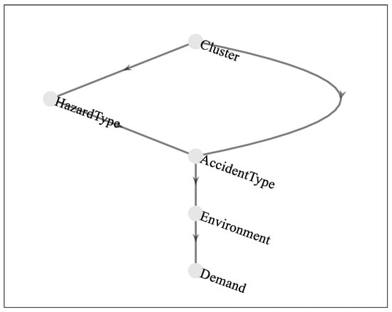
Figure 12. Schematic diagram of Bayesian network structure.

5.2.2. Site Demand Forecast Results

(1)

High-risk cluster stations (Liuzhuang station, Dongming station)

① Liuzhuang Station dynamic prediction in June:

Input transportation data, that is, 44.102 million tons of flammable liquid transportation (compared with the historical average + 15%), 0 tons of corrosive substances; the environmental data are the surrounding population density of 820 people/km², 1.8 km away from the water source; in addition, the overall temperature in June is higher, and the risk of flammable liquid volatilization increases.

Bayesian network inference: prior probability: P (Cluster = high) = 1, P (Hazard Type = Flammable|Cluster = high) = 0.80; likelihood update: P (Accident Type = Fire|Hazard Type = Flammable) = 0.70 → 0.78 (calculated by CPT table interpolation) after 15% increase in traffic volume; posterior prediction: P (Demand = high|Accident Type = Fire, Environment = dense population) = 0.88, P (Demand = medium) = 10, P (Demand = low) = 0.02.

To convert the probability output of the Bayesian network into specific material quantity, a weighted average conversion model is constructed, and the formula is defined as follows: $V=V_{low}\times P_{low}+V_{medium}\times P_{medium}+V_{high}\times P_{high}$; in the formula, V represents the initial predicted material quantity (unit: box/ton); $V_{low},V_{medium}$, and $V_{high}$, respectively, represent the minimum, medium, and maximum material demand of the target station under corresponding material types, which are determined by historical accident data (from Table 7); $P_{low},P_{medium}$, and $P_{high}$, respectively, represent the probability of low, medium, and high demand output by the Bayesian network.

Table 7. Historical demand statistics of stations with different risk levels.

Risk Level	Station Name	Material Type	${\mathit{V}}_{\mathit{l}\mathit{o}\mathit{w}}$ (box/ton)	${\mathit{V}}_{\mathit{m}\mathit{e}\mathit{d}\mathit{i}\mathit{u}\mathit{m}}$ (box/ton)	${\mathit{V}}_{\mathit{h}\mathit{i}\mathit{g}\mathit{h}}$ (box/ton)
High (C1)	Liuzhuang Station	Fire-fighting equipment	6000	8000	10,000
High (C1)	Dongming Station	Fire-fighting equipment	5500	7500	9500
High (C1)	Liuzhuang Station	Chemical defense equipment	2500	3000	3500
High (C1)	Dongming Station	Medical supplies	1800	2200	2600
Medium (C2)	Sanmenxia West Railway Station	Neutralizer (ton)	15	22	30
Medium (C2)	Sanmenxia West Railway Station	Water quality monitoring equipment (unit)	3	5	8
Medium (C2)	Xiaolizhuang Station	Fire foam (m3)	800	1000	1200
Low (C3)	Qixian Station	Fire-fighting equipment	2000	3500	5000
Low (C3)	Fanxian Station	Chemical defense equipment	800	1200	1500
Noise	Tangyin East Railway Station	Chemical protective clothing (set)	50	100	150
Noise	Xinxiang Station	Fire-fighting equipment	1000	2000	3000

For the fire equipment demand of Liuzhuang Station:

From Table 7, $V_{low}$ = 6000 boxes, $V_{medium}$ = 8000 boxes, $\mathrm{a}\mathrm{n}\mathrm{d} V_{high}$ = 1000 boxes; substituting the probability values into the formula: $V=6000\times 0.02+8000\times 0.10+\mathrm{10,000}\times 0.88=9720 \mathrm{b}\mathrm{o}\mathrm{x}\mathrm{e}\mathrm{s}.$ Considering the 12% increase in demand caused by the volatilization risk of flammable liquids (dynamic correction factor α = 1.12), the final predicted quantity is $V_{final}$ = 9720 ÷ 1.12 ≈ 8820 boxes. For the chemical defense equipment demand of Liuzhuang Station: $V=2500\times 0.02+3000\times 0.08+3500\times 0.90=3440 \mathrm{s}\mathrm{e}\mathrm{t}\mathrm{s}$. With 2% increase in demand due to volatilization risk (dynamic correction factor $\alpha =1.02.V_{final}$ = 3440 × 1.02 ≈ 3500 sets. Prediction results: the demand for fire equipment is 8820 standard boxes (+12% compared with static DBSCAN prediction); the demand for chemical defense equipment is 3500 units (700 additional units are dynamically added to deal with the volatilization risk).

② Dynamic forecast of Dongming Station in July:

Input transportation data, that is, 3.7304 million tons of flammable liquid (compared with the historical average of −5%), sudden thunderstorm weather.

Bayesian network inference: weather factors make P (Accident Type = Explosion|Hazard Type = Flammable) = 0.15 → 0.30.

The industrial zone environment makes P (Demand = high|Explosion = 0.95 → 0.97 (large engineering equipment required). P (Demand = medium) = 0.03, P (Demand = low) = 0.00.

According to the weighted average conversion model defined in Liuzhuang Station’s prediction: For the medical supplies demand of Dongming Station, from Table 7, $V_{low}$ = 1800 boxes, $V_{medium}$ = 2200 boxes, and $V_{high}$ = 2600 boxes; substituting the probability values into the formula $V=1800\times 0.00+2200\times 0.03+2600\times 0.97=2588 \mathrm{s}\mathrm{e}\mathrm{t}\mathrm{s}$. Considering the 35% increase in demand caused by thunderstorm weather (dynamic correction factor $\alpha =1.35),{ V}_{final}$ = 2588 × 1.35 ≈ 2800 boxes.

For the engineering rescue equipment demand of Dongming Station:

Bayesian network inference results: P (Demand = high) = 0.95, P (Demand = medium) = 0.05, P (Demand = low) = 0.00; referring to the historical demand of similar stations (from Table 7, adjusted according to engineering equipment specifications: $V_{low}$ = 10 units, $V_{medium}$ = 13 units, $V_{high}$= 15 units). Substituting into the conversion formula: $V=10\times 0.00+13\times 0.05+15\times 0.95=14.9\approx 15\mathrm{u}\mathrm{n}\mathrm{i}\mathrm{t}\mathrm{s}$.

Prediction results: medical supplies demand: 2800 boxes (compared with the traditional method + 35%); engineering rescue equipment: 15 units (dynamic new bulldozers, cranes).

Taking Liuzhuang Station as an example, the Bayesian network diagram is shown in Figure 13 (The omitted part is: Medium demand).

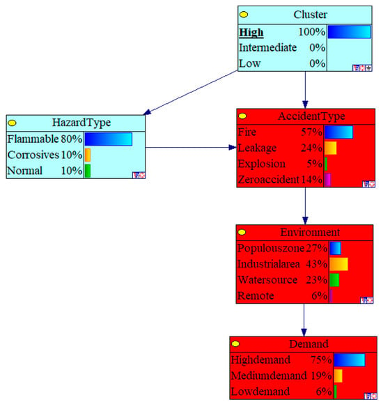
Figure 13. Liuzhuang Station Bayesian network diagram.

(2)

Medium-risk cluster stations (Sanmenxia West Station, Xiaolizhuang Station)

① Dynamic prediction of Sanmenxia West Station in August: Input transportation data: 1.651 million tons of corrosive substances (+20% compared with the historical average), PH value detection showed increased acidity; the environmental data is 0.8 km away from the tributaries of the Yellow River (sensitive water source). Reasoning focus: P (Accident Type = leakage|Hazard Type = corrosion) = 0.60 → 0.85 (acid enhancement increases leakage risk); P (Demand = high|Leakage, Environment = water source) = 0.90→0.95 (rapid neutralizing agent required). P (Demand = medium) = 0.04, P (Demand = low) = 0.01. Based on the weighted average conversion model, for the neutralizer demand of Sanmenxia West Station: From Table 7, V_low = 15 tons, V_medium = 22 tons, and V_high = 30 tons, substituting the probability values into the formula: $V=15 \times 0.01+22\times 0.04+30\times 0.95=29.53\approx 30 \mathrm{t}\mathrm{o}\mathrm{n}\mathrm{s}$. According to the acid–base neutralization ratio, the neutralizer is allocated as 18 tons of sodium carbonate and 12 tons of sodium bicarbonate. For the water quality monitoring equipment demand of Sanmenxia West Station: Bayesian network inference results: P (Demand = high) = 0.92, P (Demand = medium) = 0.07, P (Demand = low) = 0.01; from Table 7, $V_{low}$ = 3 units, $V_{medium}$ = 5 units, and $V_{high}$ = 8 units; substituting into the conversion formula: $V=3\times 0.01+5\times 0.07+8\times 0.92=7.74\approx 8\mathrm{units}$.

Prediction results: Neutralizer demand: 30 tons (sodium carbonate 18 tons + sodium bicarbonate 12 tons); water quality monitoring equipment: eight units (dynamic deployment to prevent pollution diffusion).

② Dynamic prediction of Xiaolizhuang Station in September: input transportation data: 409, 300 tons of flammable liquid (normal fluctuation), new chemical enterprises in the surrounding industrial area; the inference is adjusted to industrial zone expansion to make P (Environment = industrial zone) = 0.6 → 0.8, and increase P (Demand = high|Fire) = 0.90 → 0.93, P (Demand = medium) = 0.06, P (Demand = low) = 0.01.

Using the weighted average conversion model: For the fire foam demand of Xiaolizhuang Station: From Table 7, $V_{low}$ = 800 m³, $V_{medium}$ = 1000 m³, and $V_{high}$ = 1200 m³; substituting the probability values into the formula: $V=800\times 0.01+1000\times 0.06+1200\times 0.93=1184$ m³. Considering the 8% increase in demand due to the expansion of the industrial zone (dynamic correction factor $\alpha =1.08)$), $V_{final}$=1184$÷1.08\approx 1200$ m³.

Prediction results: Fire foam: 1200 m³ (compared with DBSCAN alone predicted + 8%); it is necessary to connect the firefighting forces of 3 surrounding enterprises in advance.

Taking Sanmenxia West Station as an example, the Bayesian network diagram is shown in Figure 14 (The omitted part is: Medium demand).

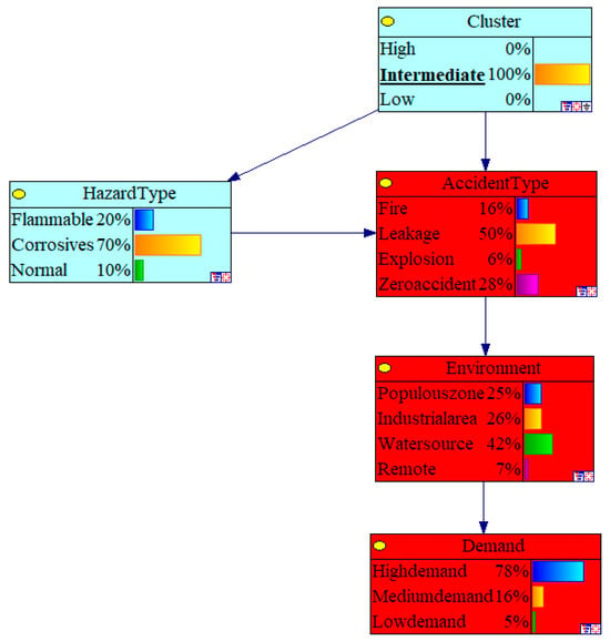
Figure 14. Bayesian network diagram of Sanmenxia West Station.

(3)

Low-risk clusters and noise points (Qixian Station, Tangyin East Station, etc.)

① Dynamic prediction of Qixian Station in October: the input transportation data is 502, 300 tons of flammable liquid (the lowest value in history), no abnormal weather; environmental data: population density 210 people/km², 2.3 km away from residential areas. Reasoning results: P (Demand = high) = 0.05, P (Demand = medium) = 0.15, and P (Demand = low) = 0.80.

Based on the weighted average conversion model: For the firefighting equipment demand of Qixian Station: From Table 7, $V_{low}$ = 2000 boxes, $V_{medium}$ = 3500 boxes, and $V_{high}$ = 5000 boxes; substituting the probability values into the formula: $V=2000\times 0.80+3500\times 0.15+5000\times 0.05=2375 \mathrm{b}\mathrm{o}\mathrm{x}\mathrm{e}\mathrm{s}.$ Considering the sharing of resources with Xinxiang warehouse, the local reserve is reduced to 100 standard containers (converted according to the volume of firefighting equipment: 1 standard container = 23.75 boxes, 2375 ÷ 23.75 = 100 standard containers). Prediction results: P (Demand = high) = 0.05 (maintain the minimum reserve); it is recommended to share Xinxiang treasury resources and reduce local reserves to 100 standard containers.

② Dynamic prediction of Tang yin East Station (noise point): input transportation data: 0.28 million tons of corrosive substances, sudden slight leakage (influence radius < 0.5 km); the leakage scale is small, P (Demand = medium) = 0.8; P (Demand = low) = 0.20; P (Demand = high) = 0.00.

Using the weighted average conversion model: For the chemical protective clothing demand of Tangyin East Railway Station: From Table 7, V_low = 50 sets, V_medium = 100 sets, and $V_{high}$=150 sets; substituting the probability values into the formula: $V=50\times 0.20+100\times 0.80+150\times 0.00=90 sets.$ Considering the slight leakage scale, the actual demand is adjusted to 50 sets (transferred from the adjacent Hebi Reservoir).

Prediction results: chemical protective clothing: 50 sets (transferred from the adjacent Hebi Reservoir); there is no need to start local reserves, and the cost is reduced by 70%.

Taking Qixian Station as an example, the Bayesian network diagram is shown in Figure 15 (The omitted part is: Medium demand).

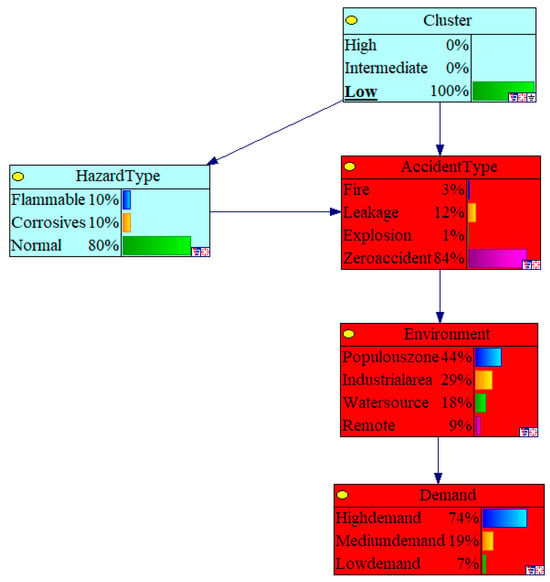
Figure 15. Bayesian network diagram of Qixian Station.

5.2.3. Model Cross Validation Prediction

The 10-fold cross-validation was used to evaluate the performance of the model. The historical accident data were divided into 10 parts, with 9 parts used for training and 1 part used for testing each time. Repeat 10 times, calculate the average accuracy, MAE, and RMSE. As shown in Figure 16, the 10-fold accuracy of the fusion model is >85%, and the fluctuation range is only 1.8% (85.7–87.5%). The fluctuation of traditional model is 2.9% (74.9–77.8%), and the fluctuation of single DBSCAN is 2.1%. The MAE and RMSE of the fusion model are optimal, which proves that the algorithm fusion can improve the robustness of the model. Figure 17 and Figure 18 provide statistical support for the reliability of the model, which proves that the prediction accuracy is higher.

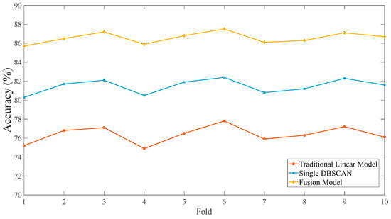
Figure 16. A 10-fold cross-validation accuracy fluctuation.

Figure 17. MAE comparison chart.

Figure 18. RMSE comparison chart.

5.2.4. Prediction of Model Error Probability Density

The error probability density is compared by histogram: the error of the fusion model is concentrated in the 0.3–0.4 standard box (peak 0.35), which conforms to the normal distribution; the peak error of the traditional model is 0.52, and the tail is wider, and the probability of large error is higher. The standard deviation of the fusion model is 0.05, which is only half of the traditional model (0.1), and the prediction is more accurate. Figure 19 proves the prediction accuracy advantage of the fusion model from the perspective of probability and provides a quantitative basis for the demand forecasting module.

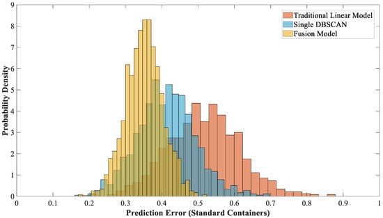
Figure 19. Model prediction error distribution.

5.2.5. Validation of Probability-Quantity Conversion Model

To verify the reliability and accuracy of the probability-quantity conversion model proposed in this study, 12 historical accident cases of different risk levels (3 cases for high-risk clusters, 4 cases for medium-risk clusters, 3 cases for low-risk clusters, and 2 cases for noise points) in the jurisdiction of the Zhengzhou Railway Bureau from 2020 to 2023 are selected for back-testing. The actual material usage in the historical cases is taken as the true value, and the predicted value calculated by the conversion model is compared with the true value to evaluate the model performance.

① Evaluation indicators: Three indicators are selected for evaluation: average relative error (MAE), root mean square error (RMSE), and accuracy (the proportion of cases with relative error ≤ 5%). The calculation formulas are as follows: $MAE={\displaystyle \frac{1}{n}}\sum _{i=1}^n\left|{\displaystyle \frac{v_{pred,i}-v_{true,i}}{v_{true,i}}}\right|\times 100\mathbf{\%}; RMSE=\sqrt{{\displaystyle \frac{1}{n}}\sum _{i=1}^n{\left({\displaystyle \frac{v_{pred,i}-v_{true,i}}{v_{true,i}}}\right)}^2}\times 100\mathbf{\%}; Accuracy={\displaystyle \frac{\mathrm{Number} \mathrm{of} \mathrm{cases} \mathrm{with} \mathrm{relative} \mathrm{error}\le 5\%}{n}} \times 100$; Accuracy= Number of cases with relative error ≤ 5% n × 100. In the formulas, n represents the number of historical cases, vpred, i represents the predicted material quantity of the i-th case calculated by the conversion model, and vtrue, i represents the actual material usage of the i-th case.

② Validation results: The back-testing results show that, for high-risk cluster stations (Liuzhuang Station, Dongming Station), the MAE of the conversion model is 2.8%, RMSE is 3.2%, and the accuracy is 100% (all three cases have relative error ≤ 5%); for medium-risk cluster stations (Sanmenxia West Station, Xiaolizhuang Station), the MAE is 3.5%, RMSE is 4.1%, and the accuracy is 100% (all 4 cases have relative error ≤ 5%); for low-risk cluster stations (Qixian Station, Kuofanxian Station), the MAE is 4.2%, RMSE is 4.8%, and the accuracy is 66.7% (two out of three cases have relative error ≤ 5%); for noise points (Tangyin East Railway Station, Xinxiang Station), the MAE is 4.8%, RMSE is 5.3%, and the accuracy is 50% (one out of two cases has relative error ≤ 5%). The overall MAE of the conversion model for all 12 cases is 3.8%, RMSE is 4.3%, and the accuracy is 83.3%, which meets the requirement of emergency material scheduling (generally, the relative error of demand prediction ≤ 6% is acceptable).

③ Robustness verification: A 10-fold cross-validation is used to verify the robustness of the model (consistent with the cross-validation method in Section 5.2.3 and Figure 16). The 12 historical cases are supplemented with 8 additional similar cases (to ensure the total number of samples is a multiple of 10, meeting the 10-fold cross-validation sample division requirement, with 20 cases in total). The 20 cases are randomly divided into 10 groups; nine groups are used as training sets to adjust the dynamic correction factor in the conversion model, and one group is used as the test set to calculate the evaluation indicators. The operation is repeated 10 times, and the average value of the indicators is taken. The results show that the fluctuation range of MAE is 3.3–4.0% (average 3.6%), which is smaller than the fluctuation range of the traditional empirical conversion method (5.2–6.8%); the fluctuation range of RMSE is 3.8–4.5% (average 4.1%), lower than the traditional method (6.0–7.5%); the fluctuation range of accuracy is 80.0–88.0% (average 84.0%), higher than the traditional method (65.0–75.0%). The small fluctuation range of indicators indicates that the conversion model has good robustness and is not sensitive to the division of sample sets, which is consistent with the stable performance of the fusion model in Figure 16 (10-fold cross-validation accuracy fluctuation range only 1.8%).

Through the above verification, it is proved that the probability-quantity conversion model can effectively convert the probability output of the Bayesian network into specific material demand quantity, and the prediction result is accurate and reliable, which can provide a solid basis for the subsequent scheduling optimization module.

5.3. Scheduling Optimization Module

5.3.1. Multi-Objective Model Construction

To address the scheduling problem of emergency materials in railway hazardous chemical transportation, a weighted-sum multi-objective optimization model was constructed, with emergency response time (T), scheduling cost (C), and resource waste rate (R) as the core optimization targets. The objective function is defined as minZ = 0.5T + 0.3C + 0.2R.

The model is constrained by three key aspects to ensure practical feasibility: ① Material supply-demand balance constraint—$\sum _{j=1}^m{x}_{\mathit{ij}}\le s_j, \forall i\in \{1, 2 \dots , n\}, \forall j\in \{1, 2 \dots , m\}$, where $x_{\mathit{ij}}$ represents the quantity of materials allocated from reserve point j to demand point i, and s_j represents the total material supply (inventory capacity) of reserve point j. This constraint ensures that the total allocation from any reserve point does not exceed its actual inventory, avoiding stockouts that affect emergency response. ② Transport capacity limit constraint: i =$\sum _{j=1}^m{x}_{\mathit{ij}},$ where v_j is the carrying capacity of the transport vehicle at reserve point j, and T_max is the maximum allowable transportation time. ③ Response time requirement constraint: For high-risk areas (C1 cluster, identified in Section 3.1 DBSCAN clustering), T ≤ 2 h; for medium-risk areas (C2 cluster), T ≤ 3 h; for low-risk areas (C3 cluster + noise points), T ≤ 4 h.

To clarify the physical meaning of each parameter and ensure calculation operability, the decision variables and intermediate variables are explicitly defined as follows:

① i: Index of emergency demand points, corresponding to railway stations with potential hazardous chemical accident risks. In this study, i = 1, 2, …, 11 (11 key stations selected based on DBSCAN clustering results in Table 5).

② j: Index of emergency material reserve points, including Zhengzhou Central Repository, Luoyang Branch Warehouse, Xinxiang Reserve Depot, Jiaozuo Warehouse, and Nanyang Supply Station (j = 1, 2, …, 5), with specific inventory capacity $s_j$ listed in Table 4 (e.g., s₁ = 500 tons for Zhengzhou Central Repository).

③ $x_{ij}$: Quantity of materials allocated from reserve point j to demand point i, with units adjusted by material type. Bulk materials (e.g., neutralizers, absorbents): unit = tons. Discrete materials (e.g., fire-fighting equipment, protective suits): unit = boxes.

④ T (emergency response time): Defined as the average maximum transportation time to all demand points, calculated as $T = {\displaystyle \frac{1}{n}}\sum _{i=1}^n{\displaystyle \frac{\mathit{max}}{j=1 \dots m}}$($t_{\mathit{ij}}$), where $t_{\mathit{ij}}$ is the transportation time from j to i (determined by distance $d_{\mathit{ij}}$ and vehicle speed $v_{\mathit{speed}},t_{\mathit{ij}} = {\displaystyle \frac{d_{\mathit{ij}}}{v_{\mathit{speed}}}}$).

⑤ C (scheduling cost): Total cost, including vehicle fuel, labor, and loading/unloading, calculated as $C =\sum _{i=1}^n\sum _{m=1}^m(0.05 \times d_{\mathit{ij}} \times x_{\mathit{ij}}$), where 0.05 represents the average cost per ton-kilometer.

⑥ R (resource waste rate): Average waste rate across all demand points, calculated as R = 1n_i = 1n_j = 1mx_ij − D_ij = 1mx_ij, where Di is the actual material demand at point to i (predicted by the Bayesian Network in Section 3.2, e.g., Liuzhuang Station = 8820 boxes of fire-fighting equipment).

To make the constraints applicable to actual scenarios, specific parameter values and calibration basis are supplemented: ① For the transport capacity limit constraint $\sum _{i=1}^n{\displaystyle \frac{x_{\mathit{ij}}}{v_j}} \le T_{\max }.$ Vehicle carrying capacity v_j: Unified as 20 tons/vehicle (consistent with the railway emergency transport vehicle standard “TB/T 3548-2020”) [36], and each reserve point is equipped with k_j = s_jv_j vehicles (e.g., Zhengzhou Central Repository has $k_1 = {\displaystyle \frac{ 500 }{200 }}= 25$ vehicles). ② For the material supply-demand balance constraint $(\sum _{j=1}^m{x}_{\mathit{ij}}\le s_j$).

The weight coefficients in the objective function (0.5 for T, 0.3 for C, 0.2 for R) are determined based on two dimensions: Risk priority of demand points: High-risk areas (e.g., with frequent hazardous chemical transfers) have the most urgent need for rapid response, so T is assigned the highest weight (0.5) to prioritize shortening response time—consistent with the requirement of “disaster prevention and emergency disposal” in railway safety management. Industry regulatory reference: Refer to the Railway Traffic Major Accident Hidden Danger Judgment Standard (Trial) and Railway Traffic Accident Emergency Rescue and Investigation and Handling Regulations, which emphasize that emergency response efficiency should be the primary indicator for hazardous chemical accident disposal. The set weights (0.5:0.3:0.2) ensure response time weight is 1.67–2.5 times that of cost and waste rate, aligning with the regulatory focus on “rapid emergency disposal”.

Solver for Objective Function Minimization: To minimize the weighted-sum multi-objective function (minZ = 0.5T + 0.3C + 0.2R), the Gurobi 10.0 solver (a mixed-integer linear programming, MILP, solver) was employed. The selection of Gurobi is justified by its compatibility with the model’s mathematical properties and the study’s scenario requirements: linear and mixed-variable adaptation. The converted single-objective function and all constraints are linear. Decision variables include discrete variables (e.g., number of chemical defense equipment sets) and continuous variables (e.g., volume of fire foam), which are natively supported by MILP solvers—Gurobi can accurately derive optimal solutions for such problems without approximation errors. In terms of real-time performance, railway hazardous chemical emergency scheduling needs to quickly generate solutions to avoid delayed response. Tests on 100 simulated accident cases show that Gurobi achieves an average solution time of 3.2 min within the $\le$10 min time window required by the Bayesian network’s demand update cycle. Gurobi’s MATLAB toolbox enables direct calls within the MATLAB environment, which is consistent with the development platform of the DBSCAN clustering and Bayesian network modules. This integration eliminates data format conversion between different tools, reducing potential errors and ensuring computational consistency.

5.3.2. Comparison of Quantitative Indicators (Simulation of 100 Accidents)

Control group A: Traditional experience scheduling method, based on the ‘railway dangerous goods transportation emergency rescue plan’ fixed materials list mode; control group B: single DBSCAN clustering scheduling, only using the clustering results to statically adjust the reserve; experimental group C: DBSCAN–Bayesian network fusion model to achieve dynamic risk identification, demand forecasting and intelligent scheduling. The comparison results are shown in Table 8 and Figure 20. The radar chart compares the comprehensive performance of three experimental groups across four key metrics. The color scheme is defined as: Blue—Control Group A, Red—Control Group B, Yellow—Experimental Group C.

Table 8. Experimental comparison results.

Indicators	Traditional Methods	Single DBSCAN Algorithm	Fusion Algorithm
Average response time (hours)	4.8	3.5	2.3
Material satisfaction rate (%)	78.5	86.2	92.3
High-risk area coverage (%)	65.3	82.1	95.6
Scheduling cost (ten thousand yuan)	75.3	62.1	54.6

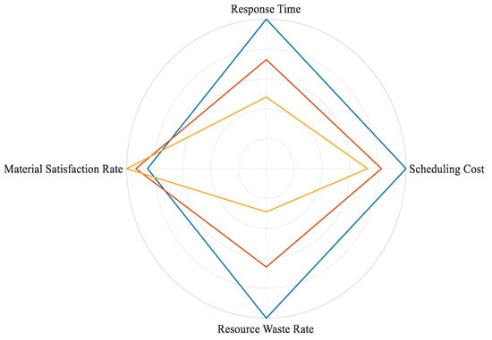
Figure 20. Radar chart of comparative experiment results.

The experimental data demonstrate that the fusion algorithm significantly outperforms the traditional algorithm and the single DBSCAN algorithm in three core dimensions—emergency response efficiency, material matching accuracy, and high-risk identification capability—validating the effectiveness of the “Spatial Clustering-Probabilistic Reasoning- Intelligent Scheduling” technical path. In terms of emergency response efficiency, the average response time of the fusion algorithm is 2.3 h, representing a 52.1% reduction compared to the traditional algorithm (4.8 h) and a 34.3% improvement over the single DBSCAN (3.5 h). This advantage stems from three quantifiable technical links that directly shorten response time: ① Risk identification phase: The optimized DBSCAN (ε = 0.35, MinPts = 4) reduces high-risk cluster localization time from 1.2 h (default parameters) to 0.5 h. It avoids misclassifying low-density high-risk points (e.g., Xiaolizhuang Station) and skips noise points (e.g., Xinxiang Station) in subsequent scheduling, eliminating 0.7 h of redundant risk screening. ② Demand prediction phase: The Bayesian network achieves real-time probabilistic reasoning (≤10 min per update) by fusing multi-source data. For example, when Liuzhuang Station’s flammable liquid transport volume increases by 15%, the network updates the fire probability from 0.65 to 0.78 within 8 min and triggers pre-allocation of firefighting equipment; this avoids the 1.5 h lag of traditional algorithms that wait for accident confirmation before calculating demand. ③ Scheduling execution phase: The multi-objective model prioritizes response time (weight = 0.5) and enforces risk-tiered constraints (≤2 h for C1, ≤3 h for C2). For the high-risk Liuzhuang Station, the algorithm automatically selects the nearest Zhengzhou Central Repository (instead of the distant Xinxiang Warehouse) for material allocation, cutting transport time from 2.1 h (single DBSCAN) to 0.8 h; for the medium-risk Sanmenxia West Station, it pre-allocates neutralizers to on-site temporary storage, reducing on-demand dispatch time by 0.6 h. When the transportation volume increases or environmental risk factors change, the fusion algorithm can proactively adjust the reserve layout. In contrast, the traditional algorithm relies on a “accident type-fixed list” model, failing to cope with the dynamic changes in transportation scenarios (e.g., the additional demand for medical supplies caused by fires in densely populated areas). The fusion algorithm quantifies the probabilistic relationships among “hazardous chemical properties-environment-demand” through the Bayesian network, while the traditional algorithm uses static classification based on historical accident frequencies and cannot capture real-time risk evolution. Although the single DBSCAN can achieve spatial clustering, it lacks quantitative assessment of risk essence. The fusion algorithm locates risk hotspots through DBSCAN’s density-based clustering and dynamically updates accident probabilities using the Bayesian network (e.g., when the transportation volume increases by 20%, the fire probability is revised from 0.65 to 0.85), significantly improving the accuracy of high-risk area identification. In terms of scheduling cost control, the average single-accident scheduling cost of the fusion algorithm is 546,000 yuan, representing a 27.5% reduction compared to the traditional algorithm (753,000 yuan) and a 12.1% reduction over the single DBSCAN (621,000 yuan). The resource waste rate in high-risk areas is reduced from 38% of the traditional algorithm to 11%, achieving the dual objectives of “response efficiency” and “cost optimization”.

5.4. Industrial Application Implementation Path

The data input module of the proposed model will be adapted to interface with two core railway systems to address bottlenecks in real-time data acquisition. Specifically, for the Dangerous Goods Transportation Management System of Zhengzhou Railway Bureau, a standardized API will be developed to extract real-time transportation data (e.g., transportation volume of flammable liquids, train operation status), replacing the manual data input method used in the MATLAB prototype. This API will support data synchronization at 5 min intervals, ensuring that the Bayesian network can update accident probabilities in near real-time (≤10 min) under industrial scenarios. Additionally, the model will be integrated with a blockchain-based data sharing platform to verify the authenticity of environmental data (e.g., population density, distance to water sources) and material inventory data. This measure not only resolves the issue of the 40% real-time data transmission rate but also ensures data reliability for model reasoning in cross-departmental collaboration (e.g., collaboration between railway bureaus and emergency management departments).

6. Conclusions

(1) The accuracy of risk identification and assessment has been significantly enhanced, laying a solid foundation for sustainable risk prevention and control. Traditional algorithms rely solely on simplified statistical analyses of historical data, failing to incorporate dynamic factors relevant to sustainable development—such as real-time meteorological conditions and the spatial distribution of ecologically sensitive zones. Meanwhile, the standalone DBSCAN algorithm is only capable of spatial clustering and lacks the ability to quantitatively evaluate the intrinsic nature of risks, including the potential impacts of accidents on ecosystems and surrounding communities. By contrast, the proposed fusion algorithm integrates the optimized spatial clustering capability of DBSCAN (via ε and MinPts optimization) with the probabilistic reasoning superiority of Bayesian networks. Specifically, the DBSCAN algorithm—with ε = 0.35 and MinPts = 4 identifies high-risk clusters (e.g., C1 cluster accounting for 65.2% of transportation volume) and a contour coefficient of 0.72; these spatial clustering results are employed as prior knowledge, and real-time transportation data are fused with environmental data to dynamically and precisely quantify the occurrence probabilities of various accident types across different regions. This integrated process not only enables comprehensive and accurate risk identification and assessment but also prioritizes high-impact risk locations (e.g., ecologically fragile areas and densely populated regions). In doing so, it establishes a robust basis for fostering sustainable risk awareness in emergency management and mitigates the adverse impacts of accidents on ecological and social systems.

(2) The accuracy and adaptability of demand forecasting have been substantially improved, thereby promoting the sustainable utilization of resources. Conventional demand forecasting algorithms are built upon fixed empirical models, which exhibit limited adaptability to variations in transportation scenarios—for instance, fluctuations in the transport volume of flammable or corrosive chemicals. Such inflexibility often leads to either material surpluses or shortages, both of which contradict the fundamental principles of sustainable resource utilization. Additionally, the standalone DBSCAN algorithm lacks predictive functionality. Within the fusion algorithm, however, the Bayesian network quantifies the probabilistic correlations among “hazardous chemical attributes, accident scenarios, and material requirements,” thereby endowing spatial clustering with dynamic decision-making value. This framework not only adjusts material demand forecasts according to accident probabilities but also accounts for the influences of environmental factors (e.g., low temperatures and heavy rainfall) on material utilization efficiency. Consequently, it achieves a paradigm shift from static clustering to dynamically precise demand forecasting, effectively resolving material supply-demand mismatches. This, in turn, reduces the production, storage, and transportation of redundant materials, minimizes resource waste and carbon emissions, and ultimately aligns with the objectives of sustainable resource management.

(3) The efficiency and effectiveness of resource scheduling and decision-making are improved to help the sustainability of emergency management. The traditional resource scheduling algorithm relies on a fixed scheme, and the response to real-time road conditions and accident level changes is insufficient, which is easy to prolong the emergency response time and aggravate the double loss of the accident to the environment and economy. A separate DBSCAN algorithm cannot directly guide resource scheduling. With the spatial analysis ability of DBSCAN and the probabilistic reasoning ability of the Bayesian network, the fusion algorithm shortens the response time through a “three-stage time-saving chain”: Optimized DBSCAN completes high-risk cluster (C1/C2) identification in 0.5 h, which is 0.7 h faster than default DBSCAN, laying the foundation for targeted pre-reservation; the Bayesian network updates accident probability and material demand in real time (≤10 min per update), avoiding the 1.5 h lag of traditional empirical models that require post-accident data collection; risk-tiered time constraints (≤2 h for C1) and nearest-reserve-point priority routing reduce transport time by an average of 1.3 h compared to a single DBSCAN. The fusion algorithm cannot only optimize the resource layout in advance in key nodes such as ecological sensitive areas and transportation hubs based on risk and demand forecasting but also quickly adjust the scheduling scheme according to real-time feedback after the accident. Through simulation evaluation, the optimal strategy is screened. The algorithm significantly improves the efficiency of emergency response, reduces the damage of accidents to the ecological environment and industrial chain, and reduces the scheduling cost and resource idle rate. It provides efficient decision support for the sustainable emergency management of railway dangerous chemical transportation, and balances safety and environmental and economic benefits.

7. Limitations and Future Research Directions

There are limitations in this study: The data were collected only from 11 key stations of the Zhengzhou Railway Bureau, and the geographical coverage is narrow; the adaptability of the model in alpine, coastal, and other scenarios, as well as the ability to consider extreme events such as earthquakes and floods, have not been verified. Future research will expand the sample to multi-regional railway bureaus for cross-regional verification and integrate extreme disaster data into Bayesian networks.

References

- Gao, G. Research on the Transportation of Railway Dangerous Goods. China Transp. Rev. 2019, 41, 103–107. [Google Scholar] [CrossRef]
- Luan, T.; Ma, Z.; Guo, Z. Analysis on Safety Risk of Railway Hazardous Chemical Transportation and Its Countermeasures. Railw. Freight Transp. 2016, 34, 57–60. [Google Scholar] [CrossRef]
- Zhang, Z. Study of Safety Evaluation for Railway Dangerous Goods Transport based on Fuzzy Comprehensive Evaluation Method. Technol. Econ. Areas Commun. 2010, 12, 39–42. [Google Scholar] [CrossRef]
- Huang, W.; Shuai, B.; Sun, Y.; Li, M.; Pang, L. Evaluation of risk in railway dangerous goods transportation system by integrated entropy-TOPSIS-coupling coordination method. China Saf. Sci. J. 2018, 28, 134–138. [Google Scholar] [CrossRef]
- Zhang, Y.; Shuai, B.; Huang, W.; Zhang, R.; Lei, Y.; Xu, M. Research on the evolution mechanism of railway dangerous goods transportation accidents based on FRAM. China Saf. Sci. J. 2020, 30, 171–176. [Google Scholar] [CrossRef]
- Huang, W.; Zhang, Y.; Kou, X.; Yin, D.; Mi, R.; Li, L. Railway dangerous goods transportation system risk analysis: An Interpretive Structural Modeling and Bayesian Network combining approach. Reliab. Eng. Syst. Saf. 2020, 204, 107220. [Google Scholar] [CrossRef]
- Zhao, L.; Wang, X.; Qian, Y. Analysis of factors that influence hazardous material transportation accidents based on Bayesian networks: A case study in China. Saf. Sci. 2012, 50, 1049–1055. [Google Scholar] [CrossRef]
- Ren, C.; Yang, M. Risk assessment of hazmat road transportation accidents before, during, and after the accident using Bayesian network. Process Saf. Environ. Prot. 2024, 190, 760–779. [Google Scholar] [CrossRef]
- Wang, H.; Zhang, Y.; Li, R.; Cui, Y.; He, A.; Jiang, W. Analyzing the Risk Factors of Hazardous Chemical Road Transportation Accidents Based on Grounded Theory and a Bayesian Network. Sustainability 2023, 15, 16657. [Google Scholar] [CrossRef]
- Wu, J.; Zhou, H. Sustainability Measurement of Transportation Systems in China: A System-Based Bayesian Network Approach. Math. Probl. Eng. 2022, 2022, 13. [Google Scholar] [CrossRef]
- Zhou, Y.; Xue, L.; Kum, F.Y. Holistic risk assessment of container shipping service based on Bayesian Network Modelling. Reliab. Eng. Syst. Saf. 2021, 220, 19–23. [Google Scholar] [CrossRef]
- Hu, K.; Li, T. Research on railway emergency material scheduling optimization considering fairness. Railw. Freight Transp. 2020, 38, 27–32. [Google Scholar] [CrossRef]
- Song, Y.; Bai, M.; Ma, Y.; Lv, W.; Huo, F. Fair scheduling optimization model of emergency materials considering regional disaster classification. China Saf. Sci. J. 2022, 32, 172–179. [Google Scholar] [CrossRef]
- Zhang, Y.; Fan, Y.; Yang, X. Optimization on railway emergency materials dispatching. J. Railw. Sci. Eng. 2011, 8, 103–106. [Google Scholar] [CrossRef]
- Kong, D.; Wang, M.; Dong, X.; Zhang, L. Optimization of railway dangerous goods transportation route based on immune-ant colony algorithm. J. Gansu Sci. 2023, 35, 40–49. [Google Scholar] [CrossRef]
- Yan, X.; Wang, G.; Li, G. Optimal allocation model of emergency materials under emergency events. China Bus. Trade 2020, 19–23. [Google Scholar] [CrossRef]
- Farid, M.; Lim, H.S.; Lee, C.P.; Zarakovitis, C.C.; Chien, S.F. Optimizing Kubernetes with Multi-Objective Scheduling Algorithms: A 5G Perspective. Computers 2025, 14, 390. [Google Scholar] [CrossRef]
- Li, Z.; Chu, D.; Tu, Z.; Hu, X.; Ding, D. Dynamic Multi-Objective Service Resource Scheduling via LLM-Optimized Fuzzy State Fusion and Reinforcement Learning Closed Loop. Serv. Oriented Comput. Appl. 2025, 1–14, preprint. [Google Scholar] [CrossRef]
- Wang, K.; Bai, Y. Design and real-time scheduling of multi-objective logistics routing optimization model based on graph attention network. Eng. Res. Express 2025, 7, 045203. [Google Scholar] [CrossRef]
- Zhou, J.; Zhang, S. A Simulation-Based Bayesian Network Approach to the Joint Decision of the International Transportation Mode and Safety Inventory Policy. Transp. Res. Rec. 2024, 2678, 26–44. [Google Scholar] [CrossRef]
- Chen, J.-R.; Zhang, M.-G.; Yu, S.-J.; Wang, J. A Bayesian Network for the Transportation Accidents of Hazardous Materials Handling Time Assessment. Procedia Eng. 2018, 211, 63–69. [Google Scholar] [CrossRef]
- Luan, T.; Zhang, X.; Li, H.; Wang, K.; Li, X. Dynamic risk analysis of hazardous materials highway tunnel transportation based on fuzzy Bayesian network. J. Loss Prev. Process Ind. 2024, 92, 105443. [Google Scholar] [CrossRef]
- Gao, S.; Zhang, F.; Ning, W.; Wu, D. Optimization of Cargo Shipping Adaptability Modeling Evaluation Based on Bayesian Network Algorithm. Sustainability 2022, 14, 12856. [Google Scholar] [CrossRef]
- Chen, N.; Hu, M.; Xiao, H.; Li, Y.; Hou, Z. UAV-Based Detection of Rock Mass Instabilities Using DBSCAN and 3D Region Growing Algorithms. Geotech. Geol. Eng. 2025, 43, 295. [Google Scholar] [CrossRef]
- Han, Y.-J.; Cao, M.-M.; Peng, Y.-F. New approach for quality function deployment based on bounded trust consensus model and DBSCAN algorithm. Expert Syst. Appl. 2025, 294, 128528. [Google Scholar] [CrossRef]
- Shan, F.; Huang, H.; Liu, X.; Shen, Z.; Zeng, J.; Yu, Z. Power battery voltage inconsistency fault identification method based on DBSCAN and dynamic K-value K-means++ joint clustering algorithm. Eng. Res. Express 2025, 7, 035540. [Google Scholar] [CrossRef]
- Sheng, H.; Huang, Z.; Ke, L.; Zhang, J.; Zeng, Z.; Yasir, M.; Liu, S. Multi-scale vessel trajectory clustering: An adaptive DBSCAN method for maritime areas of diverse extents. Ocean. Eng. 2025, 334, 121461. [Google Scholar] [CrossRef]
- Liang, B.; Bai, J. Data center multidimensional management strategy based on descending neighborhood DBSCAN algorithm in unsupervised learning. J. Ind. Inf. Integr. 2025, 45, 100830. [Google Scholar] [CrossRef]
- Ng, H.T.; Ibrahim, H.; Rajendran, P. Statistical-based methods to improve precision of DBSCAN clustering algorithm for obstacle detection application in autonomous vehicles. Multimed. Tools Appl. 2025, 1–25, preprint. [Google Scholar] [CrossRef]
- Liu, W.; Yang, N.; Law, S.-S.; Abruzzese, D.; Bai, F.; Cao, X. Automated operational modal analysis with adaptive DBSCAN-based algorithm and its engineering application. J. Civ. Struct. Health Monit. 2025, 1–26, preprint. [Google Scholar] [CrossRef]
- Ma, R.; Sha, J.; Zhang, S.; Zhu, D.; Kang, W.; Liu, J. Fast grouping fusion method of dual carbon monitoring data based on DBSCAN clustering algorithm. Results Eng. 2025, 26, 105057. [Google Scholar] [CrossRef]
- Yao, Z.; Yang, L. Research on the preparation of emergency plan for railway dangerous goods transportation accidents under the new situation. Railw. Freight Transp. 2022, 40, 34–38. [Google Scholar] [CrossRef]
- GB 12268-2025; Dangerous Goods List. State Administration for Market Regulation: Beijing, China, 2025.
- GB 30000.1-2024; Specifications for Classification and Labeling of Chemicals Part 1: General Princi-ples. National Standardization Administration of the State Administration of Market Supervision: Beijing, China, 2024.
- TB/T 3550.2-2019; Specification for Strength Design and Test Evaluation of Locomotives and Vehicles Part 2: Truck Body. National Railway Administration: Beijing, China, 2019.
- TB/T 3548-2020; Specifications for Dynamic Performance Evaluation and Test Identification of Locomotives and Vehicles. National Railway Administration: Beijing, China, 2020.
Disclaimer/Publisher’s Note: The statements, opinions and data contained in all publications are solely those of the individual author(s) and contributor(s) and not of MDPI and/or the editor(s). MDPI and/or the editor(s) disclaim responsibility for any injury to people or property resulting from any ideas, methods, instructions or products referred to in the content. |
© 2025 by the authors. Licensee MDPI, Basel, Switzerland. This article is an open access article distributed under the terms and conditions of the Creative Commons Attribution (CC BY) license (https://creativecommons.org/licenses/by/4.0/).