Abstract
Accurate runoff simulation and prediction are crucial for water resources management, especially under the impact of climate change. In this study, a multi-physics ensemble Bayesian model averaging (MPE-BMA) model is developed to improve runoff prediction accuracy by integrating a soil and water assessment tool (SWAT), hydrologiska byråns vattenbalansavdelning (HBV) model, and Bayesian model averaging (BMA) into a general framework. The MPE-BMA model integrates the strengths of the SWAT and HBV models. This approach enhances the robustness of simulation outputs and reduces uncertainties from single-model methods. MPE-BMA is subsequently employed to simulate and predict runoff for the upper reaches of Xiangxi River Basin (XXRB) in China, where four general circulation models (GCMs) and three shared socioeconomic pathways (SSP126, SSP245, and SSP585) are considered. Multiple statistical metrics (R2, NSE, and RMSE) prove that the MPE-BMA model outperforms the single models of SWAT and HBV. Results reveal that higher-emission scenarios generally lead to significant decreases in runoff, particularly by the 2080s. Specifically, under SSP585, runoff is projected to decrease by approximately 4.61–12.68% by the 2040s and 5.96–11.28% by the 2080s compared to the historical period. From the perspective of monthly and seasonal runoff changes, the peak runoff is projected to shift from June to May by the 2080s. Additionally, under SSP585, spring and summer runoffs tend to significantly increase, while winter runoff decreases sharply, leading to wetter summers and drier winters. These findings underscore the importance of enhancing water use efficiency, upgrading hydropower stations, and implementing watershed management practices to ensure sustainable water resources management in the XXRB amidst climate change.
1. Introduction
Accurate and reliable runoff prediction is crucial for making informed strategies regarding water resources management and disaster risk reduction [1,2,3]. The failure to predict runoff accurately has led to devastating consequences, as seen in several real-world events. For example, between 17 and 23 July 2021, Zhengzhou City in Henan Province was struck by devastating floods caused by unprecedented rainfall, which led to severe damage to both life and property. The State Council’s disaster response team reported that nearly 14.8 million people were affected across 150 counties and that the direct economic damage was estimated at CNY 120.06 billion [4]. In 2024, Europe experienced its most widespread flooding since 2013, with approximately 30% of the river network affected. These floods resulted in at least 335 deaths, impacted over 410,000 people, and caused economic losses exceeding EUR 18 billion. [5].
Climate change alters precipitation and evapotranspiration, affecting the distribution of water resources over time and space [6,7,8]. The Intergovernmental Panel on Climate Change’s Sixth Assessment Report (IPCC AR6) has indicated that the global surface temperature from 2011 to 2020 has been 1.1 °C higher than that from 1850 to 1900 [9]. Furthermore, the global climate is undergoing warming, and trends and uncertainties are intensifying [10,11]. This will undoubtedly increase the complexity of runoff variation, thereby exacerbating the urgency of water security issues as well as jeopardizing agricultural safety and ecological well-being [12,13,14]. Consequently, it is imperative to pursue research into the precise prediction of runoff in the context of global climate change.
Several global and regional studies have shown significant changes in runoff patterns. These changes include alterations in the timing, intensity, and magnitude of river discharge, driven by shifts in precipitation, temperature, and evapotranspiration. For example, Bai and Zhao analyzed runoff changes in China and the impacts of climate change and land use changes on runoff fluctuations, indicating that, from 1961 to 2018, the annual runoff in China showed a significant increasing trend (p < 0.05), with a rate of change of 0.4 mm per year. The study found that climate change contributed 54% to the observed changes in runoff [15]. Gray et al. conducted grid-based runoff and urban runoff predictions, suggesting that future hydrological climate conditions would be largely determined by the climate scenarios in key runoff-producing regions, such as Southeast Asia, the Amazon Basin, and mountainous areas outside of the United States [16]. Song et al. argued that changes in climate factors, particularly precipitation and potential evapotranspiration, were the primary drivers of hydrological changes in China. They found that climate change has resulted in a reduction in runoff by 7.6 mm per year [17]. Wu et al. found that since the 1990s, surface runoff in Central Asia has been decreasing, with 44.6% of the region’s decline primarily driven by reduced snowmelt and 33.2% driven by decreased precipitation [18].
Hydrological models are regarded as crucial tools for runoff prediction, which are broadly categorized into data-driven models (DDMs) and physically based models (PBMs). DDMs have been frequently employed in runoff prediction, including artificial neural networks (ANNs), support vector machines (SVMs), and other machine learning and deep learning models [19,20,21,22]. DDMs boast advantages in their extensive applicability, robust adaptability, and flexible deployment because there is no requirement for modeling detailed physical processes within the watershed [23,24]. However, DDMs are constrained by limited generalizability, a high reliance on data quality, poor interpretability, and susceptibility to overfitting. While these models may offer accurate predictions under specific conditions, they may exhibit instability when faced with unknown scenarios [25,26,27]. In comparison, PBMs based on fluid mechanics and hydrology demonstrate strong generalizability. They facilitate predictive scenarios for future hydrological trends due to their reliability in generating precise physical equations under appropriate parameterization and data input conditions. Numerous PBMs grounded in different assumptions and parameterizations have been utilized for runoff prediction, such as SWAT, HEC-HMS, VIC, HBV, and MIKE-SHE [28,29,30,31]. Among these PBMs, SWAT and HBV are recognized as the two most prevalent models, lauded for their availability and capability to simulate hydrological processes rapidly and accurately [32,33,34].
In fact, different hydrological models exhibit diverse parameters and physical mechanisms. Each model emphasizes specific aspects in the interpretation and generalization of hydrological processes, thus producing varied outputs from the same inputs. It is challenging for a single model to adequately represent watershed hydrological processes. Fortunately, several studies have devised a range of techniques to ensemble the simulation results of different models to enhance prediction accuracy, such as a simple average ensemble (SAE), a weighted average ensemble (WAE), gene expression programming (GEP), a neural network ensemble (NNE), and Bayesian theory techniques. For example, Huang et al. employed an SAE in HBV and SWAT hydrological models to predict runoff in the upper reaches of the Yangtze River, suggesting that the integration of HBV and SWAT can reduce uncertainty in future projections [35]. Esmaeili-Gisavandani et al. coupled SWAT, HBV, and three other hydrological models using GEP to simulate the flow of the Hablehroud River in north-central Iran [36]. The results showed that the GEP-based hybrid model significantly improved the performance of the individual models. Gelete et al. integrated SWAT, HBV, and the Hydrologic Engineering Center-Hydrologic Modeling System (HEC-HMS) using the NNE technique. The results indicated that in the validation phase, the NNE technique improved the performance of SWAT, HBV, and HEC-HMS by 12.14%, 22.7%, and 26.8%, respectively [37]. Li et al. employed Bayesian theory to integrate information from four global climate models (GCMs) under four SSP-RCP climate scenarios, indicating that multi-model integration significantly enhanced data accuracy and reduced the impact of uncertainty on climate change prediction [38]. Zhou et al. combined long short-term memory networks, Bayesian theory, and transfer learning techniques to predict the maximum water depth and flood time series using different meteorological inputs [39]. The integrated model reduced the average relative error from 9.5% to 0.76%, significantly enhancing model compatibility and generalization. In general, ensembled techniques have demonstrated strong prediction and simulation performance, with the application of Bayes’ theorem growing rapidly.
Bayesian model averaging (BMA), developed based on Bayesian theory, is a highly representative method for ensemble prediction. BMA achieves a weighted average of multiple models, with weights estimated based on the posterior model probability. BMA assigns weights based on model performance. This reduces the risks of single-model reliance and improves prediction reliability. Recently, BMA has gained substantial popularity across various scientific disciplines. Moknatian et al. introduced BMA to integrate the simulation results of the SWAT-Hillslope model (SWAT-HS) calibrated with different objective functions, showing that the prediction intervals of multi-objective functions encompassed 94–97% of the observed values, significantly surpassing the performance of single-objective functions [40]. Wei et al. employed BMA to integrate comprehensive precipitation data from four datasets; the results demonstrated a 14% improvement in the accuracy of the integrated dataset compared to the individual datasets [41]. Zhou et al. utilized the time-varying BMA (TV-BMA) method to combine the results of three machine learning models for predicting urban floods and warnings. The results demonstrated that the predictive accuracy of the TV-BMA model was 11.4–50.4% higher than that of individual models [42]. Li et al. applied BMA to integrate the forecasting results of LSTM, GRU, and TCN in Panyang Lake. This approach resulted in a 21% improvement in the Nash–Sutcliffe efficiency (NSE) compared to individual models [43]. Generally, BMA is an ideal choice for ensemble prediction in multiple physical hydrological models as it can reduce uncertainty and provide more comprehensive information for decision-making.
Therefore, this study aims to develop a multi-physics ensemble Bayesian model averaging (MPE-BMA) model for runoff simulation and prediction by integrating SWAT, HBV, and BMA into a general framework. The developed MPE-BMA model has merit in leveraging the strengths of both SWAT and HBV to aggregate the simulation outputs, thereby enhancing prediction accuracy by offsetting the simulation errors of individual models. Then, MPE-BMA will be applied to the upper reaches of the Xiangxi River Basin (XXRB) in China to verify its practicality. The results are expected to improve the simulation and prediction accuracy of runoff in the XXRB, which will provide more effective support for future water resources management.
2. Material and Methods
2.1. Study Area
The upper reach of the Xiangxi River Basin (XXRB) is located in western Hubei Province, China (110°47′–111°13′ E, 30°96′–31°59′ N). Covering a catchment area of 3099 km2 (Figure 1), the basin is characterized by high and sub-high mountains. The dominant land use type is forest, which covers 87.36% of the watershed. The region experiences a tropical semi-humid climate, with mild temperatures and abundant rainfall throughout the year, although the temperature can exceed 30 °C in summer. The average annual temperature is approximately 17.1 °C, and precipitation ranges from 900 to 1200 mm annually, decreasing from northwest to southeast. The rainy season spans from June to September, with heavy rainfall often causing rapid changes in river levels. The flood season starts in April and lasts until October, followed by a dry season. From 1991 to 2008, the historical runoff showed a slight declining trend. Given the critical role that runoff plays in water resources management, agriculture, and disaster risk reduction, studying the hydrological processes in the XXRB is essential for developing strategies to address future water-related challenges.
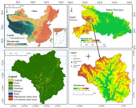
Figure 1.
Study area with hydrological and meteorological stations.
2.2. MPE-BMA Framework
Figure 2 presents the framework of the MPE-BMA model, consisting of four main steps: (i) data collection and preprocessing, (ii) development of the MPE-BMA model, (iii) projections of future temperature and precipitation using the statistical downscaling model (SDSM), and (iv) prediction of future runoff using the MPE-BMA model. The SWAT and HBV models simulate hydrological processes based on specified input data, each emphasizing different aspects of the hydrological cycle. To enhance the accuracy of runoff simulation, the outputs from both models are ensembled using the Bayesian model averaging (BMA) method. The MPE-BMA model does not merge the physical mechanisms of the SWAT and HBV models, but instead combines the simulation outputs of the two independent hydrological models through the Bayesian model averaging (BMA) method. The SWAT and HBV models simulate runoff processes separately based on their respective physical structures, preserving the integrity of their individual hydrological processes. The BMA method statistically synthesizes the outputs by assigning different weights to each model’s predictions according to their predictive performance and associated uncertainties. Future runoff is then predicted using the MPE-BMA model, with SDSM providing higher-resolution projections of climate variables, including temperature and precipitation.
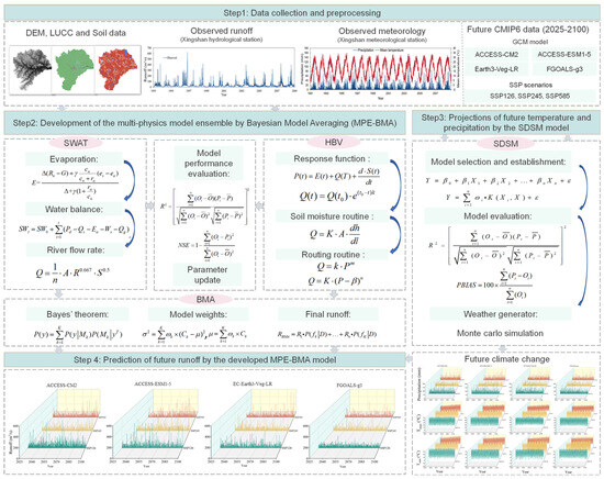
Figure 2.
Framework of the MPE-BMA model.
2.2.1. SWAT Model and Input Data
SWAT, a widely utilized process-driven distributed hydrological model, is selected for its excellent performance in simulating soil infiltration and analyzing geographical topography [44]. The SWAT model can divide the watershed into a series of sub-basins and decompose complex ecological and hydrological processes into manageable units through the integration of sub-models for different scales of simulation and analysis [45]. The water balance equation in SWAT is essential for understanding the distribution and movement of water within a watershed. It considers various hydrological components to simulate the comprehensive water cycle. The water balance equation in SWAT is given by:
where represents the final soil moisture content; t is the calculation duration; denotes the initial soil moisture content; indicates the daily rainfall; , , and denote the daily surface runoff, evapotranspiration, and subsurface runoff, respectively; and represents the daily lateral infiltration and leakage in the soil profile. can be calculated using the Manning equation [46]:
where n stands for the channel roughness coefficient, which signifies the resistance of water flow within the channel; A denotes the sub-watershed area; R represents rainfall, typically expressed in terms of c units; and S refers to the slope.
The SWAT model requires several key inputs, including the digital elevation model (DEM), land use, soil type, meteorological data, and runoff data. Table 1 provides detailed data sources and preprocessing steps. The spatial data consistencies of the DEM, land use, and soil data are ensured by utilizing GIS tools. The flow network is generated using flow direction and flow accumulation calculations, and rivers are extracted based on a predefined flow accumulation threshold to determine the outlet points of the watershed. Sub-basin subdivision is automatically completed based on the river network and control points, with the option to manually adjust the control points to meet research needs. This study divided the entire watershed into 29 sub-watersheds and generated the boundary layer for each. Further HRU subdivision is performed within sub-basins based on factors such as land use, soil type, and slope, further subdividing the hydrological response units.

Table 1.
Data sources and corresponding processing.
After preparing the input data, the SWAT model is calibrated and validated using the SWAT-CUP tool, an automated parameter estimation tool that facilitates calibration and sensitivity analysis. Initially, sixteen parameters are selected for analysis. Following sensitivity analysis using Sequential Uncertainty Fitting Version 2 (SUFI-2), ten parameters are identified as relatively sensitive for subsequent research, thus enhancing the model’s calibration efficiency. Table 2 lists the descriptions, initial ranges, and optimal ranges of the parameters. Optimized parameters are estimated based on daily runoff data from the Xingshan hydrological station. Model calibration is conducted using 10 years of data from 1993 to 2002, while model validation employs 6 years of data from 2003 to 2008. Additionally, a 2-year warm-up period from 1991 to 1992 is utilized for model initialization to ensure that the model reaches a stable state before calibration. The model is calibrated using data from 1993 to 2002 by adjusting parameters to fit the observed runoff. Validation is performed using independent data from 2003 to 2008 to assess model performance.
Table 2.
Parameters and optimal values of the SWAT model for the XXRB.
2.2.2. HBV Model and Input Data
HBV is a process-driven, semi-distributed conceptual and daily time-step hydrological model. The simplicity of its structure and relatively low input data requirements allow the HBV model to excel in small watersheds and real-time forecasting [47,48]. It provides timely runoff estimates through its rapid response to precipitation events, which is crucial for streamflow forecasting and water resources management. The fundamental principle of the HBV model is rooted in water balance, which is described as [48]:
where Q represents the total runoff, n denotes the time-step number for precipitation, which includes both rainfall and snowfall components, Ei represents evaporation, S1i and S2i denote the water volumes in the runoff storage reservoirs, and U signifies the baseflow.
The construction and parameter tuning of the HBV model are performed using the HBV-light software version 4.0.24 (https://www.geo.uzh.ch/en.html, accessed on 14 May 2025). The input of the HBV model includes daily precipitation, temperature, and evapotranspiration, which are from the Xingshan meteorological station. According to the requirements of the HBV model, the XRBB is divided into five elevation zones and three vegetation zones based on land use and DEM data. For parameter tuning, the Monte Carlo method is employed to generate a set of parameter values within the specified range. After 50,000 iterations, the optimal set of model parameters under given conditions is determined. The frequency distribution plot of Reff values is shown in Figure S1, which is included in the Supplementary Materials. The descriptions, initial ranges, and optimal ranges of the selected parameters are presented in Table 3. The calibration and validation periods for HBV are consistent with those set for the SWAT model.
Table 3.
Sensitive parameters and optimal values of the HBV model for the XXRB.
2.2.3. BMA
BMA combines the predictions of multiple models into a comprehensive forecast using a weighted averaging method in Bayesian inference. The prediction results of each model are weighted according to its posterior probability, which reflects the model’s reliability given the current observed data. Through this weighting, BMA can balance the strengths and weaknesses of different models, reducing the bias or errors that a single model might introduce. BMA reduces bias and variance, enhancing the robustness of the model and providing more stable and accurate predictions. This approach helps mitigate the risk of overfitting and improves predictive performance [49]. In detail, the relationship between posterior (prediction) probability distribution functions (PDFs) and prior (ensemble) PDFs can be defined by Bayes’ theorem, which is given as follows [50]:
where denotes the correct posterior probability of model fk given the observed data, reflecting the fit between model fk and the observed data. In BMA, the weights are crucial because they reflect the plausibility of each model given the observed data. The posterior mean and variance of the BMA prediction can be expressed as [51]:
where is the variance associated with model prediction fk with respect to the observed data. The final BMA prediction for a new output is:
In the equation, Rn represents the simulation result of the n-th model. When the total of posterior probabilities equals 1, they can be considered as the weight of each model. In the BMA framework, we used different likelihood functions and compared their performance. By comparing the AIC and BIC values of the models, we ultimately decided to use the Pearson type III distribution. The AIC and BIC values of the specific likelihood functions are shown in Table S1. Then, the weights of the SWAT and HBV models were determined based on their posterior probabilities, which are calculated using their fit to the observed runoff data. The model with a higher posterior probability, indicating better performance in reproducing the observed data, is assigned a greater weight in the final BMA prediction. The weights of the SWAT and HBV models are finally determined using Matlab, and are 0.613 and 0.387, respectively.
2.2.4. SDSM and Future Meteorological Data
To bridge the gap between GCM outputs and the localized information needed for runoff prediction, downscaling is an essential process in climate modeling [52]. SDSM is widely used for enhancing the accuracy of climate data due to its moderate data requirements, flexibility, ease of integration with GCMs, and high performance [53]. The selected GCMs are listed in Table 4. In this study, the sixth version of SDSM 4.2.9 is used to downscale the CMIP6 data to generate high-resolution climate data for the XXRB from 2025 to 2100, including the maximum temperature, minimum temperature, and daily precipitation. The detailed procedure is as follows:
Table 4.
The selected global climate models (GCMs) of CMIP6.
(i) The stepwise multiple linear regression (SMLR) method is used to select the optimal independent variables from 26 atmospheric NCEP forecast variables, ultimately identifying four variables. Then, the statistical relationships between observed meteorological data at local stations and selected NCEP variables are investigated within the basin.
(ii) The calibration period for the SDSM model is from 1993 to 2002, and the validation period is from 2003 to 2008. The model’s accuracy is evaluated using the coefficient of determination (R2).
(iii) Future climate data from GCMs are then input into the established SDSM to generate future climate data.
2.2.5. Model Performance Evaluation
The performances of SWAT, HBV, SDSM, and MPE-BMA are typically assessed based on the comparison of observed and simulated runoffs. In this study, the statistical metrics of R2, NSE, and RMSE are employed to quantify the model’s performance [54,55]. The detailed information is shown in Table 5.
Table 5.
Model performance evaluation indicators.
3. Results and Discussion
3.1. Hydrological Model Performance Evaluation
Figure 3 presents the comparison of runoff simulation performance among the SWAT, HBV, and MPE-BMA models. In the calibration period, the HBV model achieves an R2 of 0.74, an NSE of 0.72, and an RMSE of 14.71 m3/s. The SWAT model slightly outperforms HBV with an R2 of 0.77, an NSE of 0.74, and an RMSE of 14.24 m3/s. However, the MPE-BMA model demonstrates superior performance with an R2 of 0.81, an NSE of 0.79, and a significantly lower RMSE of 11.94 m3/s. During the validation period, the HBV model’s performance metrics are an R2 of 0.71, an NSE of 0.71, and an RMSE of 16.24 m3/s. The SWAT model again shows slightly better performance with an R2 of 0.73, an NSE of 0.72, and an RMSE of 13.71 m3/s. The MPE-BMA model continues to outperform both individual models with an R2 of 0.78, an NSE of 0.76, and an RMSE of 12.13 m3/s. To demonstrate the performance of the MPE-BMA model, we compared the results from previous studies that applied SWAT, HBV, and other hydrological models to runoff prediction within the Xiangxi River Basin (XXRB). Liu et al. examined the impact of different land use data on runoff outputs from the SWAT model in the XXRB, reporting optimal R2 and NSE values of 0.77 and 0.65, respectively, during the validation period [56]. Similarly, Wang et al. explored the baseline method for runoff forecasting using the SWAT model in the XXRB, achieving optimal R2 and NSE values of 0.73 and 0.72, respectively, during the validation period [57]. These results indicate that, during both the calibration and validation periods, the MPE-BMA model provided higher accuracy in runoff simulation compared to previously reported studies. As a result, the MPE-BMA model demonstrates superior performance and is considered more suitable for future runoff predictions, offering enhanced reliability and accuracy.
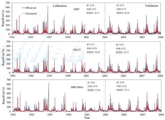
Figure 3.
Daily simulated and observed runoffs during the calibration and validation periods.
3.2. Future Climate Change Scenarios Using SDSM Downscaling Simulations
The performance of SDSM is evaluated using R2 for daily precipitation, maximum temperature (Tmax), and minimum temperature (Tmin). During the validation period (2005–2008), the R2 for precipitation is 0.53. In contrast, the R2 values for Tmax and Tmin are 0.91 and 0.93, respectively. The results highlight the SDSM’s strong capability in generating high-resolution Tmax and Tmin. Although the simulation of precipitation is more challenging due to its complex and stochastic nature, SDSM still demonstrates a reasonable ability to simulate precipitation in the XXRB [58,59]. Figures S2–S4 show the projections of Tmax, Tmin, and precipitation from 2025 to 2100 using SDSM for four GCMs and three SSP scenarios. The results indicate significant variability in the projections of Tmax, Tmin, and precipitation. To reflect the changes of Tmax, Tmin, and precipitation compared to the reference period of 1991–2008, the projection time is divided into two timeframes for the 2040s (2025–2059) and the 2080s (2060–2100). The changes in the climate projections with respect to the reference period are illustrated in Figure 4. The changes in Tmax and Tmin exhibit a clear upward trend across all GCMs and SSPs, with more pronounced increases under SSP585. Precipitation changes are more variable, showing both increases and decreases depending on the GCMs and SSPs.
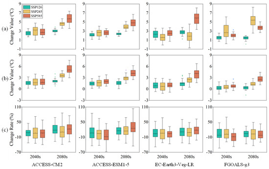
Figure 4.
Changes of (a) Tmax, (b) Tmin, and (c) precipitation relative to the reference period (1991–2008) under different climate scenarios.
In terms of Tmax, the increase is significant under SSP585 in both the 2040s and 2080s, with the most pronounced changes occurring in the 2080s, where projected changes exceed 8.13 °C for some GCMs. Specifically, the EC-Earth3-Veg-LR model exhibits the highest increase in Tmax under SSP585, with changes of 3.12 °C in the 2040s and 6.81 °C in the 2080s, while the ACCESS-ESM1-5 model shows more moderate increases of 2.48–5.51 °C across all SSPs during both periods. Tmin follows a similar trend, with substantial increases under SSP585 and moderate increases under SSP126 and SSP245 in both the 2040s and 2080s. The ACCESS-CM2 model demonstrates the highest increases in Tmin, particularly under SSP585, with changes of 6.81 °C in the 2040s and 3.12 °C in the 2080s. The daily precipitation projections show a wide range of changes across both time periods. In the 2040s, some GCMs project increases of up to 86.87%, while others project decreases, reflecting the complexity and uncertainty of precipitation patterns. The ACCESS-ESM1-5 model exhibits a significant increase in precipitation under SSP585, with changes of 44.11%, whereas the ACCESS-CM2 model shows notable decreases under SSP126, with changes of −32.59%. In the 2080s, the variability in precipitation projections persists, with some GCMs projecting increases of up to 103.37% and others projecting decreases of similar magnitudes. The ACCESS-ESM1-5 model exhibits the most significant increase in precipitation under SSP585, with changes of 49.29%, while the FGOALS-g3 model shows notable decreases in precipitation under SSP126, with changes of −36.28%. Overall, Tmax and Tmin show a continuous upward trend, with the increase becoming more pronounced under stronger emission scenarios. Precipitation is projected to decrease in the 2040s, but this reduction is expected to be mitigated by the 2080s. These projected changes in Tmax, Tmin, and precipitation are critical for predicting future runoff patterns and will significantly impact runoff dynamics.
3.3. Runoff Responses to Future Climate Change
Future runoff in the XRBB is predicted by the MPE-BMA model. Figure 5 shows the predicted runoff from 2025 to 2100 for four GCMs and three SSPs during the 2040s and 2080s. The runoff trends are analyzed using the Sen slope and the Mann–Kendall (M-K) trend test, which are presented in Table 6. The Sen slope quantifies the trend magnitude, while the M–K value indicates the statistical significance of the trend [60,61]. A positive Sen slope indicates increasing runoff trends, while a negative slope indicates decreasing trends. Z-values categorize the trend significance, with higher absolute values reflecting stronger significance.
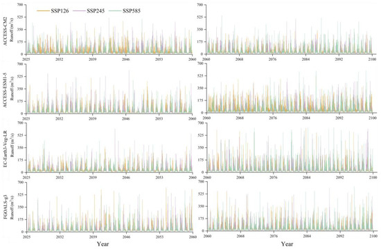
Figure 5.
Predicted runoff under different climate scenarios.
Table 6.
Results of the Sen slope and the M–K trend test for predicted runoff.
In Table 6, the results indicate that higher-emission scenarios generally lead to highly significant decreases in runoff, which is particularly evident in the 2080s. For example, in the 2080s, ACCESS-CM2 shows a highly significant decrease in runoff under SSP585, with a Sen slope of −0.46 m3/s and a Z-value of 10.75. For the same period, SSP245 shows a decrease, with a Sen slope of −0.36 m3/s and a Z-value of 11.46. Conversely, lower-emission scenarios exhibit mixed trends. For ACCESS-ESM1-5 under SSP126, there is a highly significant increase in runoff in the 2040s and 2080s, with Sen slopes of 0.28 m3/s and 0.35 m3/s and Z-values of 7.33 and 7.41, respectively. In comparison, FGOALS-g3 shows a highly significant decrease in the 2040s, with a Sen slope of −0.92 m3/s and a Z-value of 10.05, but a highly significant increase in the 2080s, with a Sen slope of 0.50 m3/s and a Z-value of 5.97. Generally, climate change has potentially adverse impacts on future runoff. The results highlight significant variability across GCMs and timeframes, showing the complexity of runoff prediction under climate change. The most significant decrease in runoff is observed for ACCESS-CM2 under SSP585 in the 2080s with a Sen slope of −0.46 m3/s and a Z-value of 10.75. On the other hand, the most significant increase in runoff is seen for FGOALS-g3 under SSP126 in the 2080s, with a Sen slope of 0.50 m3/s and a Z-value of 5.79. These findings highlight the critical need for adaptive water resource management strategies tailored to specific temporal and climate contexts.
Figure 6 illustrates the projected monthly runoff variations across different GCMs and SSP scenarios for the 2040s and 2080s. Each GCM exhibits a clear seasonal runoff pattern, with peak runoff typically occurring in the middle of the year (June–July) and the lowest runoff at the beginning and end of the year (December–February). From the perspective of runoff volume, peak runoff is projected to shift from June to May by the 2080s. This shift may be due to increased spring precipitation, which leads to earlier soil saturation and runoff generation. Additionally, rising temperatures enhance evaporation rates and accelerate the hydrological cycle, causing earlier peaks in runoff. Future runoff changes show significant differences under various climate scenarios. As emission intensity increases, peak runoff gradually rises, with the most pronounced change under the SSP585 scenario. In the 2040s, peak runoff in May under the SSP126, SSP245, and SSP585 scenarios is approximately 1100 m3/s, 1150 m3/s, and 1250 m3/s, respectively. By the 2080s, the peak runoff under SSP585 has increased to around 1300 m3/s, which is significantly higher than in low-emission scenarios. This indicates that peak flows during the wet season are stronger under high-emission scenarios, intensifying extreme runoff events. During dry seasons (January–February), runoff increases to varying degrees across scenarios, with the most evident rise under SSP585. Under the SSP585 scenario, the runoffs during spring and summer rise significantly, while the runoff during winter decreases more sharply, leading to wetter summers and drier winters. This is because the SSP585 scenario is characterized by more substantial increases in both temperature and precipitation. Increased precipitation during high runoff months leads to higher runoff. However, higher temperatures increase evaporation and transpiration rates, leading to reduced soil moisture and lower runoff during low rainfall months, exacerbating dry conditions. In contrast, the SSP126 and SSP245 scenarios exhibit more moderate changes, resulting in less dramatic runoff variations. These findings underscore the need for robust, adaptable water resource management strategies to address the anticipated seasonal extremes and effectively manage the uncertainties in future runoff patterns due to climate change. Additionally, establishing a robust monitoring and early warning system for extreme weather events can help mitigate the impact of floods and droughts, safeguarding both water resources and local communities.
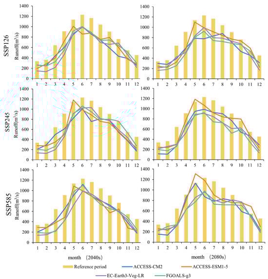
Figure 6.
Comparison of the monthly distribution of runoff under different climate scenarios during the 2040s and 2080s relative to the historical period (1993–2008).
Figure 7 presents the prediction results of annual runoff through violin and radar plots. The violin plots on the left show the distribution of annual runoff across four GCMs. The radar plots on the right provide a visual comparison of the percentage changes in annual runoff relative to the historical period. The results reveal significant variations in predicted annual runoff across different scenarios. Among these GCMs, ACCESS-ESM1-5 exhibits the largest variability in runoff predictions, indicating a higher sensitivity to emission scenarios. Conversely, other GCMs show more consistent patterns, although the extent of the reductions still varies. Comparing the SSPs, the high-emission scenario SSP585 consistently shows greater reductions in annual runoff. Specifically, under SSP585, runoff is projected to decrease by approximately 4.61–12.68% by the 2040s and 5.96–11.28% by the 2080s compared to the historical period. In contrast, the lower-emission scenarios (SSP126 and SSP245) show smaller reductions. SSP126, for example, exhibits decreases of 7.05–10.64% in the 2040s and 9.89–13.69% in the 2080s. The temporal analysis further underscores the progressive nature of these changes. Runoff decreases progressively from the historical period to the 2040s and further to the 2080s across all scenarios. This suggests that the impacts of climate change on water resources will intensify over time.
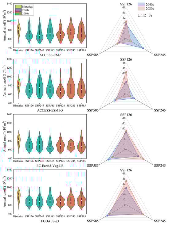
Figure 7.
Annual runoff during the 2040s and 2080s under different climate scenarios and their variation relative to the historical period (1993–2008).
Generally, these variations in annual runoff can be attributed to a complex interplay between rising temperatures and changing precipitation patterns, as shown in Figure 4. Higher temperatures can lead to increased evapotranspiration rates, reducing the amount of water available as runoff. Projected changes in precipitation directly lead to uncertainties in runoff predictions. Increased precipitation could enhance runoff, while decreased precipitation would reduce it. While the specific magnitude of runoff reductions differs among the GCMs and SSPs, all GCMs consistently indicate that higher-emission scenarios will lead to more substantial declines in water availability. Given the specific characteristics of the XXRB and the continuously decreasing runoff, several practical suggestions for sustainable water resources management are recommended. Enhancing water use efficiency would reduce dependency on seasonal rainfall and address the high demand for agricultural water, which can be achieved by introducing advanced irrigation techniques such as drip irrigation and rainwater harvesting. To ensure the sustainability of hydropower generation, existing small hydropower stations can be upgraded with more efficient turbines and energy storage solutions to better manage fluctuations in water flow. In addition, watershed management practices, including reforestation and afforestation projects, can improve water retention and reduce soil erosion, thereby stabilizing runoff patterns, especially considering the extensive forest cover in the region. These measures, tailored to the unique conditions of the XXRB, can contribute significantly to sustainable water resources management in the face of climate change.
4. Discussion
4.1. Model and Result
In this study, the MPE-BMA approach is developed for runoff prediction in the XXRB. Compared to individual hydrological models, such as SWAT and HBV, the MPE-BMA model significantly improves the accuracy of runoff predictions (as shown in Figure 3). The main advantage of MPE-BMA is its use of weighted averaging to combine outputs from different hydrological models. This approach helps overcome the limitations of individual models and results in more robust predictions. To validate the effectiveness of the MPE-BMA model in the XXRB, we compared its results with those of existing studies that applied various hydrological models, including SWAT, semi-distributed land use-based runoff processes (SLURP), the global hydrological model (GHM), catchment-scale hydrological models (CHMs), and stepwise-clustered hydrological inference (SCHI) models. Previous studies reported R2 values between 0.65 and 0.76 and NSE values between 0.54 and 0.70 [62,63,64,65,66], respectively. In comparison, the MPE-BMA model achieved an R2 of 0.81 and an NSE of 0.79, both of which are higher than the results from the referenced models. This demonstrates that the MPE-BMA model can more effectively enhance runoff prediction accuracy in the XXRB.
Our results further demonstrate the significant impact of climate change on runoff in the XXRB, with a clear decreasing trend in runoff over the coming decades, particularly under SSP585. For instance, projections for the 2040s suggest a reduction in runoff by approximately 4.61% to 12.68%. This finding aligns with the general trend observed in previous studies. However, the magnitude of the projected decrease varies across different models. For example, Gelete et al. used the GHM and CHM models and estimated that mean annual runoff relative to the baseline period (1961–1990) could potentially decrease by up to 40% [67]. In contrast, Bieger et al. applied the SWAT model and found that future runoff could decrease by approximately 10% [68]. These discrepancies highlight uncertainties in climate modeling. They also show that runoff predictions are sensitive to model structure, parameterization, and climate-forcing assumptions. Nevertheless, the consistent downward trend in runoff across these studies supports the notion that climate change is likely to exacerbate water scarcity in the XXRB. Furthermore, our study not only corroborates the global trends in climate change impacts on hydrological systems but also provides validation for the MPE-BMA model’s robustness in addressing these complex, scenario-driven changes in hydrological behavior.
4.2. Uncertainties
The uncertainties associated with the structure of the SWAT and HBV models significantly impact the accuracy of runoff predictions in the XXRB. The SWAT model, based on a physically based approach, simulates watershed hydrology using processes such as infiltration, evapotranspiration, and surface runoff. This detailed representation of land use, vegetation, and soil properties allows SWAT to capture a wide range of hydrological processes. However, this complexity makes SWAT highly sensitive to input data quality. Inaccuracies in land use and soil characteristics can cause significant errors in runoff predictions. In contrast, the HBV model adopts a simpler, conceptual approach, with lumped parameterization of hydrological processes. While it is less data-intensive and requires fewer input parameters, the HBV model may oversimplify certain processes, especially in regions with complex land–surface interactions, leading to the potential under- or over-estimation of runoff. To mitigate structural uncertainty, increasing the spatial resolution of input data and incorporating finer-scale land use and soil data could reduce the model’s dependence on simplified assumptions, improving the overall robustness of predictions [69,70].
In addition to structural uncertainty, parameter calibration in both SWAT and HBV models introduces significant uncertainty. In the SWAT model, ten key parameters, such as the SCS curve number (CN2), baseflow alpha factor (ALPHA_BF), and evapotranspiration threshold depth (REVAPMN), are identified as highly sensitive to runoff predictions. Despite the use of the SWAT-CUP tool and the Sequential Uncertainty Fitting Version 2 (SUFI-2) approach for calibration, the accuracy of parameter estimates remains variable due to the spatial heterogeneity of the watershed and temporal variations in climate data. Parameters such as CN2, which governs surface runoff, can change significantly with land use, soil type, and precipitation patterns, leading to potential errors in runoff estimates. Similarly, the HBV model was calibrated using the Monte Carlo method with 50,000 iterations. Despite this, considerable uncertainty remains, especially for sensitive parameters such as the snowmelt threshold temperature (TT) and maximum soil moisture storage (FC), which vary with land cover and elevation [71]. To reduce parameter uncertainty, applying advanced optimization techniques, such as multi-objective optimization or machine learning algorithms, can be considered to enhance the precision of parameter estimates. These methods can help better capture the complex hydrological dynamics in regions with heterogeneous data and improve the overall calibration of hydrological models [72,73].
The downscaling of climate model data using methods such as SDSM introduces uncertainty, particularly in regions with significant spatial variability in precipitation and temperature. While SDSM is effective, its ability to accurately reflect local precipitation changes is limited due to the high spatiotemporal variability of precipitation, leading to potential biases in runoff simulation. Additionally, uncertainties arise from the use of different climate models (GCMs) and climate scenarios (e.g., SSP126, SSP245, and SSP585), which result in varying predictions of future climate change and can consequently affect runoff forecasts. To reduce these uncertainties, higher-resolution climate data or comparing multiple GCMs should be utilized to minimize downscaling errors. Additionally, expanding the range of climate scenarios, especially under extreme conditions, will provide a more comprehensive assessment of the impacts of climate change on runoff.
The BMA method reduces model errors by averaging the outputs of multiple models, but the weight estimation process introduces uncertainty, particularly when models are highly correlated. BMA assumes that model errors are independent, but in cases such as SWAT and HBV, which share similar structural assumptions and outputs under similar climate scenarios, model errors may be correlated, affecting the weight estimation. Additionally, BMA’s weight calculation relies on model performance metrics (e.g., R2 and NSE), which are influenced by input data quality and model assumptions. Several advanced techniques, such as Copula-embedded BMA and segmented ensemble BMA, can be explored to allow for more flexible weight estimation and improve model integration by capturing complex non-linear relationships and model interdependencies [50].
5. Conclusions
In this study, a multi-physics ensemble Bayesian model averaging (MPE-BMA) model is developed to reduce errors in runoff simulation and achieve more accurate runoff predictions. In the MPE-BMA model, the physical hydrological models SWAT and HBV, as well as BMA and the SDSM method, are integrated into a cohesive framework. The MPE-BMA model harnesses the strengths of each individual method, thus addressing the limitations of single-model approaches and achieving greater accuracy and reliability in runoff predictions. MPE-BMA has been applied in the XXRB in China to predict long-term runoff until 2100 under four GCMs and three SSPs.
The findings can be summarized as follows: (i) MPE-BMA demonstrates superior runoff simulation accuracy, achieving an R2 of 0.78, an NSE of 0.76, and an RMSE of 12.13 m3/s during validation, outperforming the SWAT and HBV models; (ii) Tmax and Tmin in the XRBB indicate a continuous and pronounced increase under higher-emission scenarios, with significant variability in precipitation patterns, showing both increases and decreases depending on the GCMs and SSPs; (iii) runoff is projected to generally decrease, with the most significant reductions occurring under SSP585, showing decreases of approximately 4.61–12.68% by the 2040s and 5.96–11.28% by the 2080s compared to the historical period; and (iv) peak runoff is projected to shift from June to May by the 2080s, with significant increases during spring and summer and sharp decreases in winter under SSP585, highlighting the need for adaptable water resource management to address seasonal extremes and uncertainties. To mitigate decreasing runoff in the XXRB, it is recommended to improve water use efficiency through advanced irrigation and rainwater harvesting, upgrade hydropower stations, and implement watershed management practices such as reforestation to stabilize runoff and ensure sustainable water resource management.
Generally, this study demonstrates the effectiveness of the integrated MPE-BMA model for runoff prediction. Several extensions and improvements can be conducted in future studies. For instance, the current study uses only the SWAT and HBV models, which may limit the comprehensive understanding of hydrological processes. Introducing additional hydrological or statistical models can capture a wider range of processes and reduce uncertainties. In terms of model data expansion, re-analyses of meteorological data can be introduced to provide a more comprehensive representation of climate change across the entire basin. In addition, the quantification of uncertainty in the runoff prediction process needs to be further strengthened.
Supplementary Materials
The following supporting information can be downloaded at: https://www.mdpi.com/article/10.3390/su17104714/s1, Figure S1: Reff frequency histogram; Figure S2: Future precipitation projected by SDSM; Figure S3: Future Tmin projected by SDSM; Figure S4: Future Tmax projected by SDSM; Table S1: Likelihood function selection criteria.
Author Contributions
W.L.: Conceptualization, Project administration, Methodology, Investigation, Data curation, Software, Formal analysis, Writing—original draft, Writing—review and editing, Visualization. H.L.: Writing—review and editing, Validation, Software, Resources, Visualization, Project administration, Data curation. P.G.: Resources, Data curation, Formal analysis, Writing—review and editing, Visualization, Software, Writing—original draft. A.Y.: Writing—review and editing, Visualization, Validation. Y.F., Y.W., Y.S. and X.Y.: Formal analysis, Writing—review and editing. All authors have read and agreed to the published version of the manuscript.
Funding
This research was supported by the Xiamen Natural Science Foundation Youth Project (3502Z20227071) and the Natural Science Foundation of Fujian Province, China (2023J011424).
Institutional Review Board Statement
Not applicable.
Informed Consent Statement
Not applicable.
Data Availability Statement
The data sources are detailed on the websites listed in Table 1.
Conflicts of Interest
The authors declare no conflicts of interest.
References
- Wang, H.; Qin, H.; Liu, G.; Liu, S.; Qu, Y.; Wang, K.; Zhou, J. A novel feature attention mechanism for improving the accuracy and robustness of runoff forecasting. J. Hydrol. 2023, 618, 129200. [Google Scholar] [CrossRef]
- Wu, J.F.; Nunes, J.P.; Baartman, J.E.M.; Yang, D.W. Disentangling the impacts of meteorological variability and human induced changes on hydrological responses and erosion in a hilly-gully watershed of the Chinese Loess Plateau. Catena 2023, 233, 107478. [Google Scholar] [CrossRef]
- Najafi, H.; Shrestha, P.K.; Rakovec, O.; Apel, H.; Vorogushyn, S.; Kumar, R.; Thober, S.; Merz, B.; Samaniego, L. High-resolution impact-based early warning system for riverine flooding. Nat. Commun. 2024, 15, 3726. [Google Scholar] [CrossRef]
- Hsu, P.C.; Xie, J.; Lee, J.Y.; Zhu, Z.; Li, Y.; Chen, B.; Zhang, S. Multiscale interactions driving the devastating floods in Henan Province, China during July 2021. Weather. Clim. Extrem. 2023, 39, 100541. [Google Scholar] [CrossRef]
- Hermans, T.H.J.; Busecke, J.J.M.; Wahl, T.; Malagón-Santos, V.; Tadesse, M.G.; Jane, R.A.; Van De Wal, R.S.W. Projecting Changes in the Drivers of Compound Flooding in Europe Using CMIP6 Models. Earth’s Future 2024, 12, e2023EF004188. [Google Scholar] [CrossRef]
- Vieira, M.J.F.; Stadnyk, T.A. Leveraging global climate models to assess multi-year hydrologic drought. Npj Clim. Atmos. Sci. 2023, 6, 179. [Google Scholar] [CrossRef]
- He, J.; Lu, K.Z.; Fosu, B.; Fueglistaler, S.A. Diverging hydrological sensitivity among tropical basins. Nat. Clim. Change 2024, 14, 623–628. [Google Scholar] [CrossRef]
- Tian, L.; Guo, S.C.; Feng, J.W.; He, C.S. Quantifying the altitudinal response of water yield capacity to climate change in an alpine basin on the Tibetan Plateau through integrating the WRF-Hydro and Budyko framework. Catena 2024, 242, 108087. [Google Scholar] [CrossRef]
- IPCC. AR6 Synthesis Report: Climate Change 2023. In Contribution of Working Group I to the Sixth Assessment Report of the Intergovernmental Panel on Climate Change; Cambridge University Press: Cambridge, UK, 2023. [Google Scholar]
- Alshahrani, M.; Laiq, M.; Noor-ul-Amin, M.; Yasmeen, U.; Nabi, M. A support vector machine-based drought index for regional drought analysis. Sci. Rep. 2024, 14, 9849. [Google Scholar] [CrossRef]
- Li, G.; Liu, Z.; Zhang, J.; Han, H.; Shu, Z. Bayesian model averaging by combining deep learning models to improve lake water level prediction. Sci. Total Environ. 2024, 906, 167718. [Google Scholar] [CrossRef]
- Fang, X.; Pomeroy, J.W. Simulation of the impact of future changes in climate on the hydrology of Bow River headwater basins in the Canadian Rockies. J. Hydrol. 2023, 620, 129566. [Google Scholar] [CrossRef]
- Hu, Y.T.; Zhang, F.; Luo, Z.Z.; Baderldin, N.; Benoy, G.; Xing, Z.S. Soil and water conservation effects of different types of vegetation cover on runoff and erosion driven by climate and underlying surface conditions. Catena 2023, 231, 107347. [Google Scholar] [CrossRef]
- Nearing, G.; Cohen, D.; Dube, V.; Gauch, M.; Gilon, O.; Harrigan, S.; Hassidim, A.; Klotz, D.; Kratzert, F.; Metzger, A.; et al. Global prediction of extreme floods in ungauged watersheds. Nature 2024, 627, 559–563. [Google Scholar] [CrossRef]
- Bai, X.; Zhao, W. Impacts of climate change and anthropogenic stressors on runoff variations in major river basins in China since 1950. Sci. Total Environ. 2023, 898, 165349. [Google Scholar] [CrossRef]
- Gray, L.C.; Zhao, L.; Stillwell, A.S. Impacts of climate change on global total and urban runoff. J. Hydrol. 2023, 620, 129352. [Google Scholar] [CrossRef]
- Song, Z.; Xia, J.; Wang, G.; She, D.; Hu, C.; Piao, S. Climate change rather than vegetation greening dominates runoff change in China. J. Hydrol. 2023, 620, 129519. [Google Scholar] [CrossRef]
- Wu, X.; Tang, W.; Chen, F.; Wang, S.; Bakhtiyorov, Z.; Liu, Y.; Guan, Y. Attribution and Risk Projections of Hydrological Drought Over Water-Scarce Central Asia. Earth’s Future 2025, 13, e2024EF005243. [Google Scholar] [CrossRef]
- Wang, J.; Wang, X.; Lei, X.H.; Wang, H.; Zhang, X.H.; You, J.J.; Tan, Q.F.; Liu, X.L. Teleconnection analysis of monthly streamflow using ensemble empirical mode decomposition. J. Hydrol. 2020, 582, 124411. [Google Scholar] [CrossRef]
- Igaue, T.; Hayashi, R. Signatures of the uncanny valley effect in an artificial neural network. Comput. Hum. Behav. 2023, 164, 107811. [Google Scholar] [CrossRef]
- Gou, J.; Soja, B. Global high-resolution total water storage anomalies from self-supervised data assimilation using deep learning algorithms. Nat. Water 2024, 2, 139–150. [Google Scholar] [CrossRef]
- Miao, J.D.; Zhang, X.M.; Zhang, G.J.; Wei, T.X.; Zhao, Y.; Ma, W.T.; Chen, Y.X.; Li, Y.R.; Wang, Y.S. Applications and interpretations of different machine learning models in runoff and sediment discharge simulations. Catena 2024, 238, 107848. [Google Scholar] [CrossRef]
- Hartmann, A.; Goldscheider, N.; Wagener, T.; Lange, J.; Weiler, M. Karst water resources in a changing world: Review of hydrological modeling approaches: KARST WATER RESOURCES PREDICTION. Rev. Geophys. 2014, 52, 218–242. [Google Scholar] [CrossRef]
- Martinho, A.D.; Hippert, H.S.; Goliatt, L. Short-term streamflow modeling using data-intelligence evolutionary machine learning models. Sci. Rep. 2023, 13, 13824. [Google Scholar] [CrossRef] [PubMed]
- Wu, C.L.; Chau, K.W.; Li, Y.S. Predicting monthly streamflow using data-driven models coupled with data-preprocessing techniques. Water Resour. 2009, 45, 2007WR006737. [Google Scholar] [CrossRef]
- Silagyi, D.V.; Liu, D.H. Prediction of severity of aviation landing accidents using support vector machine models. Accid. Anal. Prev. 2023, 187, 107043. [Google Scholar] [CrossRef]
- Yang, H.Y.; Wang, T.H.; Yang, D.W.; Yan, Z.H.; Wu, J.F.; Lei, H.M. Runoff and sediment effect of the soil-water conservation measures in a typical river basin of the Loess Plateau. Catena 2024, 243, 108218. [Google Scholar] [CrossRef]
- Keller, A.A.; Garner, K.; Rao, N.; Knipping, E.; Thomas, J. Hydrological models for climate-based assessments at the watershed scale: A critical review of existing hydrologic and water quality models. Sci. Total Environ. 2023, 867, 161209. [Google Scholar] [CrossRef]
- Lian, X.; Hu, X.; Bian, J.; Shi, L.; Lin, L.; Cui, Y. Enhancing streamflow estimation by integrating a data-driven evapotranspiration submodel into process-based hydrological models. J. Hydrol. 2023, 621, 129603. [Google Scholar] [CrossRef]
- Liu, R.; Luo, Y.; Wang, Q.R.; Wang, Y. Time-varying parameters of the hydrological simulation model under a changing environment. J. Hydrol. 2024, 643, 131943. [Google Scholar] [CrossRef]
- Wang, M.; Bodirsky, B.L.; Rijneveld, R.; Beier, F.; Bak, M.P.; Batool, M.; Droppers, B.; Popp, A.; Van Vliet, M.T.H.; Strokal, M. A triple increase in global river basins with water scarcity due to future pollution. Nat. Commun. 2024, 15, 880. [Google Scholar] [CrossRef]
- Dash, S.S.; Sahoo, B.; Raghuwanshi, N.S. SWAT model calibration approaches in an integrated paddy-dominated catchment-command. Agric. Water Manag. 2023, 278, 108138. [Google Scholar] [CrossRef]
- López-Ballesteros, A.; Nielsen, A.; Castellanos-Osorio, G.; Trolle, D.; Senent-Aparicio, J. DSOLMap, a novel high-resolution global digital soil property map for the SWAT + model: Development and hydrological evaluation. Catena 2023, 231, 107339. [Google Scholar] [CrossRef]
- Roy, A.; Kasiviswanathan, K.S.; Patidar, S.; Adeloye, A.J. A Physics-Aware Machine Learning-Based Framework for Minimizing Prediction Uncertainty of Hydrological Models. Water Resour. Res. 2023, 59, 034630. [Google Scholar] [CrossRef]
- Huang, J.L.; Wang, Y.J.; Su, B.D.; Zhai, Y.Q. Future Climate Change and Its Impact on Runoff in the Upper Reaches of the Yangtze River Under RCP4.5 Scenario. Meteorol. Mon. 2016, 42, 614–620. [Google Scholar]
- Esmaeili-Gisavandani, H.; Lotfirad, M.; Sofla, M.S.D.; Ashrafzadeh, A. Improving the performance of rainfall-runoff models using the gene expression programming approach. J. Water Clim. Chang. 2021, 12, 3308–3329. [Google Scholar] [CrossRef]
- Gelete, G.; Nourani, V.; Gokcekus, H.; Gichamo, T. Ensemble physically based semi-distributed models for the rainfall-runoff process modeling in the data-scarce Katar catchment, Ethiopia. J. Hydroinform. 2023, 25, 567–592. [Google Scholar] [CrossRef]
- Li, J.; Li, Y.; Zhang, T.; Feng, P. Research on the future climate change and runoff response in the mountainous area of Yongding watershed. J. Hydrol. 2023, 625, 130108. [Google Scholar] [CrossRef]
- Zhou, Q.; Teng, S.; Situ, Z.; Liao, X.; Feng, J.; Chen, G.; Zhang, J.; Lu, Z. A deep-learning-technique-based data-driven model for accurate and rapid flood predictions in temporal and spatial dimensions. Hydrol. Earth Syst. Sci. 2023, 27, 1791–1808. [Google Scholar] [CrossRef]
- Moknatian, M.; Mukundan, R. Uncertainty analysis of streamflow simulations using multiple objective functions and Bayesian Model Averaging. J. Hydrol. 2023, 617, 128961. [Google Scholar] [CrossRef]
- Wei, L.; Jiang, S.; Dong, J.; Ren, L.; Liu, Y.; Zhang, L.; Wang, M.; Duan, Z. Fusion of gauge-based, reanalysis, and satellite precipitation products using Bayesian model averaging approach: Determination of the influence of different input sources. J. Hydrol. 2023, 618, 129234. [Google Scholar] [CrossRef]
- Zhou, Y.; Wu, Z.; Xu, H.; Wang, H.; Ma, B.; Lv, H. Integrated dynamic framework for predicting urban flooding and providing early warning. J. Hydrol. 2023, 618, 129205. [Google Scholar] [CrossRef]
- Li, X.; Wang, Q.; Danilov, S.; Koldunov, N.; Liu, C.; Müller, V.; Sidorenko, D.; Jung, T. Eddy activity in the Arctic Ocean projected to surge in a warming world. Nat. Clim. Chang. 2024, 14, 156–162. [Google Scholar] [CrossRef]
- Jin, X.; Jin, Y.; Du, K.; Mao, X.; Zheng, L.; Fu, D.; Qin, Y. Irrigation impacts on grassland hydrological regimes in an arid endorheic river basin. J. Hydrol. 2024, 631, 130843. [Google Scholar] [CrossRef]
- Zhang, L.; Li, X.; Han, J.; Lin, J.; Dai, Y.; Liu, P. Identification of surface water—Groundwater nitrate governing factors in Jianghuai hilly area based on coupled SWAT-MODFLOW-RT3D modeling approach. Sci. Total Environ. 2024, 912, 168830. [Google Scholar] [CrossRef]
- Cai, Y.F.; Zhang, F.; Shi, J.C.; Johnson, V.C.; Ahmed, Z.; Wang, J.G.; Wang, W.W. Enhancing SWAT model with modified method to improve Eco-hydrological simulation in arid region. J. Clean. Prod. 2023, 403, 136891. [Google Scholar] [CrossRef]
- Dimitrova-Petrova, K.; Rosolem, R.; Soulsby, C.; Wilkinson, M.E.; Lilly, A.; Geris, J. Combining static and porta-ble Cosmic ray neutron sensor data to assess catchment scale heterogeneity in soil water storage and their integrated role in catchment runoff response. J. Hydrol. 2021, 601, 126659. [Google Scholar] [CrossRef]
- Sadayappan, K.; Keen, R.; Jarecke, K.M.; Moreno, V.; Nippert, J.B.; Kirk, M.F.; Sullivan, P.L.; Li, L. Drier streams despite a wetter climate in woody-encroached grasslands. J. Hydrol. 2023, 627, 130388. [Google Scholar] [CrossRef]
- Yu, Q.; Jiang, L.; Wang, Y.; Liu, J. Enhancing streamflow simulation using hybridized machine learning models in a semi-arid basin of the Chinese loess Plateau. J. Hydrol. 2023, 617, 129115. [Google Scholar] [CrossRef]
- Zhang, Q.; Li, Y.P.; Huang, G.H.; Wang, H.; Shen, Z.Y. Bayesian analysis of variance for quantifying multi-factor effects on drought propagation. J. Hydrol. 2024, 632, 130911. [Google Scholar] [CrossRef]
- Li, H.; Zhang, Y.; Chiew, F.H.S.; Xu, S. Predicting runoff in ungauged catchments by using Xinanjiang model with MODIS leaf area index. J. Hydrol. 2009, 370, 155–162. [Google Scholar] [CrossRef]
- Eingrüber, N.; Korres, W. Climate change simulation and trend analysis of extreme precipitation and floods in the mesoscale Rur catchment in western Germany until 2099 using Statistical Downscaling Model (SDSM) and the Soil & Water Assessment Tool (SWAT model). Sci. Total Environ. 2022, 838, 155775. [Google Scholar] [CrossRef] [PubMed]
- Rahimi, R.; Tavakol-Davani, H.; Nasseri, M. An Uncertainty-Based Regional Comparative Analysis on the Performance of Different Bias Correction Methods in Statistical Downscaling of Precipitation. Water Resour Manag. 2021, 35, 2503–2518. [Google Scholar] [CrossRef]
- Giglou, A.N.; Nazari, R.; Karimi, M.; Lawrence Museru, M.; Ntow Opare, K.; Nikoo, M.R. Future eco-hydrological dynamics: Urbanization and climate change effects in a changing landscape: A case study of Birmingham’s river basin. J. Clean. Prod. 2024, 447, 141320. [Google Scholar] [CrossRef]
- Nguyen, H.H.; Peters, K.; Kiesel, J.; Welti, E.A.R.; Gillmann, S.M.; Lorenz, A.W.; Jähnig, S.C.; Haase, P. Stream macroinvertebrate communities in restored and impacted catchments respond differently to climate, land-use, and runoff over a decade. Sci. Total Environ. 2024, 929, 172659. [Google Scholar] [CrossRef]
- Liu, R.M.; Wang, Q.R.; Xu, F.; Men, C.; Guo, L.J. Impacts of manure application on SWAT model outputs in the Xiangxi River watershed. J. Hydrol. 2017, 555, 479–488. [Google Scholar] [CrossRef]
- Wang, Q.; Liu, R.; Men, C.; Guo, L.; Miao, Y. Effects of dynamic land use inputs on improvement of SWAT model performance and uncertainty analysis of outputs. J. Hydrol. 2018, 563, 874–886. [Google Scholar] [CrossRef]
- Jahanshahi, A.; Patil, S.D.; Goharian, E. Identifying most relevant controls on catchment hydrological similarity using model transferability—A comprehensive study in Iran. J. Hydrol. 2022, 612, 128193. [Google Scholar] [CrossRef]
- Zhao, G.L.; Tian, S.M.; Wang, Y.M.; Liang, R.F.; Li, K.F. Quantitative assessment methodology framework of the impact of global climate change on the aquatic habitat of warm-water fish species in rivers. Sci. Total Environ. 2023, 785, 162–686. [Google Scholar] [CrossRef]
- Rahman, A.U.; Dawood, M. Spatio-statistical analysis of temperature fluctuation using Mann–Kendall and Sen’s slope approach. Clim. Dyn. 2017, 48, 783–797. [Google Scholar] [CrossRef]
- Khalil, A. Combined use of graphical and statistical approaches for rainfall trend analysis in the Mae Klong River Basin, Thailand. J. Water Clim. Chang. 2023, 14, 4642–4668. [Google Scholar] [CrossRef]
- Xu, H.; Taylor, R.G.; Kingston, D.G.; Jiang, T.; Thompson, J.R.; Todd, M.C. Hydrological modeling of River Xiangxi using SWAT2005: A comparison of model parameterizations using station and gridded meteorological observations. Quat. Int. 2010, 226, 54–59. [Google Scholar] [CrossRef]
- Gosling, S.N.; Taylor, R.G.; Arnell, N.W.; Todd, M.C. A comparative analysis of projected impacts of climate change on river runoff from global and catchment-scale hydrological models. Hydrol. Earth Syst. Sci. 2011, 15, 279–294. [Google Scholar] [CrossRef]
- Liu, R.; Zhang, P.; Wang, X.; Chen, Y.; Shen, Z. Assessment of effects of best management practices on agricultural non-point source pollution in Xiangxi River watershed. Agric. Water Manag. 2013, 117, 9–18. [Google Scholar] [CrossRef]
- Bieger, K.; Hörmann, G.; Fohrer, N. Simulation of Streamflow and Sediment with the Soil and Water Assessment Tool in a Data Scarce Catchment in the Three Gorges Region, China. J. Environ. Qual. 2014, 43, 37–45. [Google Scholar] [CrossRef]
- Han, J.C.; Huang, G.; Huang, Y.; Zhang, H.; Li, Z.; Chen, Q. Chance-constrained overland flow modeling for improving conceptual distributed hydrologic simulations based on scaling representation of sub-daily rainfall variability. Sci. Total Environ. 2015, 524–525, 8–22. [Google Scholar] [CrossRef]
- Gelete, G.; Nourani, V.; Gokcekus, H.; Gichamo, T. Physical and artificial intelligence-based hybrid models for rainfall–runoff–sediment process modelling. Hydrol. Sci. J. 2023, 68, 13. [Google Scholar] [CrossRef]
- Bieger, K.; Hörmann, G.; Fohrer, N. The impact of land use change in the Xiangxi Catchment (China) on water balance and sediment transport. Reg. Environ. Chang. 2015, 15, 485–498. [Google Scholar] [CrossRef]
- Jiang, A.; Zhang, W.; Liu, X.; Zhou, F.; Li, A.; Peng, H.; Wang, H. Improving hydrological process simulation in mountain watersheds: Integrating WRF model gridded precipitation data into the SWAT model. J. Hydrol. 2024, 639, 131687. [Google Scholar] [CrossRef]
- Strauch, A.M.; Huang, Y.F.; Tsang, Y.P. Characterizing streamflow regimes using a distributed model for sustainable resource management in the humid tropics. J. Hydrol. 2024, 636, 131287. [Google Scholar] [CrossRef]
- Sidorenko, N.Y.; Bugaets, A.N.; Lupakov, S.Y.; Gonchukov, L.V. Impact Assessment of the Potential Evapotranspiration Method on Results of Hydrological Modeling. Water Resour. 2024, 51, 405–417. [Google Scholar] [CrossRef]
- Abbas, S.A.; Bailey, R.T.; White, J.T.; Arnold, J.G.; White, M.J.; Čerkasova, N.; Gao, J. A framework for parameter estimation, sensitivity analysis, and uncertainty analysis for holistic hydrologic modeling using SWAT+. Hydrol. Earth Syst. Sci. 2024, 28, 21–48. [Google Scholar] [CrossRef]
- Feng, D.; Beck, H.; De Bruijn, J.; Sahu, R.K.; Satoh, Y.; Wada, Y.; Liu, J.; Pan, M.; Lawson, K.; Shen, C. Deep dive into hydrologic simulations at global scale: Harnessing the power of deep learning and physics-informed differentiable models (δ HBV-globe1.0-hydroDL). Geosci. Model Dev. 2024, 17, 7181–7198. [Google Scholar] [CrossRef]
Disclaimer/Publisher’s Note: The statements, opinions and data contained in all publications are solely those of the individual author(s) and contributor(s) and not of MDPI and/or the editor(s). MDPI and/or the editor(s) disclaim responsibility for any injury to people or property resulting from any ideas, methods, instructions or products referred to in the content. |
© 2025 by the authors. Licensee MDPI, Basel, Switzerland. This article is an open access article distributed under the terms and conditions of the Creative Commons Attribution (CC BY) license (https://creativecommons.org/licenses/by/4.0/).