Abstract
The misallocation of production factors, with structural misallocation as an important aspect, is a key instigator of low total factor productivity (TFP) growth rate in China, but one important question is which structural misallocation of what factor is more serious in China. Using China’s manufacturing industrial enterprise data from 1998 to 2013, we calculated and compared the factors misallocation degree among industries, ownerships and regions. The results indicated that, the misallocation among industries was most serious, which led to a TFP loss of 8.12% annually. The misallocation among ownerships ranked second, which led to a TFP loss of 5.49%. The least degree of the misallocation recorded among provinces led to TFP loss of 3.05%. By using the relative severity index, the rank is the same. As to the capital, the misallocation among ownerships was most serious, which led to TFP loss of 4.62%. But as to the labor, the misallocation among industries was most serious, which led to TFP loss of 4.58%. Moreover, the misallocation among ownerships alleviated rapidly from 1998 to 2007, while alleviated slower among industries and regions. However, from 2008 to 2013, all three types of structural misallocation have become worse, especially in labor. These conclusions are important to identify the focus of structural reform in China.
1. Introduction
Many developing countries with high-speed growth mainly depended on substantial increase of production factors to boost their economic growth, especially in China. However, such economic growth mode is characterized by high production inputs and high energy consumption, and will lead to serious environment pollution. To change this economic development model, China must change from high inputs and high energy consumption to high quality. This high-quality development model will be characterized by higher output with less inputs, which means high productivity. The Solow economic growth model [1] has already pointed out the importance of total factor productivity (TFP) to sustainable growth, where the TFP is the portion of output contributed by some other forces such as technical progress instead of traditional factor inputs. When a country reaches a certain stage of economic development, which is called steady-state in the Solow model or is called “new normal” by some Chinese officials and scholars [2] (pp. 124–127), the continued increase of inputs has less marginal contribution to output, at this point, improving the TFP will be the main driving force of economic growth. Therefore, with China’s economy entering the “new normal”, the key for sustainable economic growth will be TFP on the supply side [3,4,5,6].
How to promote TFP? In addition to the efficiency within firms, to optimize the production factor allocation across firms also has important effects on the aggregate TFP [7,8], especially in China [9,10,11,12]. If production factors flow from the firm with a low marginal product to the one with a high marginal product, the aggregate output will be higher, and if the total amount of factors is definite, the higher aggregate output will mean higher TFP. According to Yang [11], the space for economic growth which relies on the development of firms to improve the national TFP is gradually shrinking in China, thus a new mode to optimize resources allocation is required urgently. The CEWC (Central Economic Working Conference) of CPC (Communist Party of China) in 2015 has also clearly stressed that China should rectify the distorted allocation of key factors, expand effective supply and improve TFP. Under this background, Hsieh and Klenow [9] pinpointed that the national TFP loss led to by resource misallocation among firms in China was about 80%, Shao et al. [13] even pinpointed that the misallocation among firms within industries in China has led to an overall TFP loss beyond 200%. That is, if the misallocation is rectified fully, the TFP in China will increase by 200%. Therefore, to optimize the allocation of factors will be the key to improve the national TFP and realize the sustainable economic growth.
How to optimize the allocation of factors? Structural change is a fundamental way, which is of great significance to improve China’s development [14,15]. The CEWC in 2015 also stressed that China should intensify the structural reform to rectify the distorted allocation of factors. Thus it can be seen that, the structural misallocation of production factors is a key instigator of low TFP growth rate in China. However, the structural misallocation is mainly manifested in three ways in China: the misallocation led to by the imbalance of industrial structure, the misallocation led to by ownership discrimination, and the misallocation led to by market segmentation. Therefore, it will be very important to choose the focus of structural reform through making clear that which of the three structural misallocations is the most serious.
The degree of misallocation will be an important criterion to judge their seriousness. The previous studies on quantitative analysis of misallocation degree mainly measured national TFP loss through comparing the national TFP under distorted state with that under effective state. The groundbreaking models based on this idea include the model based on the assumption of heterogeneous firms to measure the degree of resource misallocation among firms within industries [9] which is called HK model in this paper for short (HK model is the abbreviation of the model proposed by Hsieh and Klenow [9]. We use the initials of the author’s name to abbreviate the model), and the model based on the assumption of homogenous firms to measure the degree of resource misallocation among industries [16,17], which is called the Aoki model in this paper for short. Restuccia and Rogerson [18] and Hopenhayn [19] have made a comprehensive review on the resource misallocation under this idea.
Therefore, we should assess the structural misallocation degree to judge which structural misallocation is more serious. Previous studies have measured the misallocation degree from different aspects, such as the misallocation among industries, ownerships, and regions [10,20,21,22,23,24,25]. However, from what follows we can see that their measuring results were not comparable, so that we will be not able to judge the relative seriousness of different structural misallocation. For this problem, we reconstructed a better and unified model. In the unified model, the whole economy is divided into three layers: the state, the group. and the firm, where the department layer is the three structures—industry, region and ownership sector—that we will analyze in this paper. In this model, the severity of every structural misallocation can be judged not only by comparing the absolute indicator of TFP loss, but also by calculating the relative indicator of the ratio of the degree of single one structural misallocation to the degree of total misallocation. As can be seen from the followed of this paper, there are still many differences in the degree of total misallocation under different arrangements of structures, so it will be more objective and reasonable to compare the relative severity of different structural misallocation by using the relative degree indicator. Then using the manufacturing industrial firms data from 1998 to 2013 and our model, we recalculated the absolute and relative structural misallocation degree in China. So there are two contributions in this paper: Firstly, we compared and judged which structural misallocation was more serious, then put forward more objective policies; secondly, we proposed a better and unified quantitative model.
2. A Unified Framework for Measuring Misallocation Degree
2.1. Comparision of Measuring Results in Previous Literatures
The previous studies have calculated the degree of structural misallocation from different aspects in China, as shown in Table 1. In terms of the misallocation among industries, Yuan and Xie [20] pointed out that the misallocation between the agricultural sector and the nonagricultural sector had led to TFP loss of 2–18%. Chen and Hu [21] pointed out that the misallocation among subindustries within China’s manufacturing industry had led to the gross output loss of 15%, which is based on the Aoki model, but Han and Zheng [22] pointed out that this misallocation only had led to TFP loss of 4.72%, which is based on HK model. In terms of the misallocation among regions, Brandt et al. [10] through extending the HK model pointed out that this misallocation had led to TFP loss of 8% (BTZ model for short). In terms of the misallocation among ownership sectors, Jin et al. [23] pointed out that it had led to an overall TFP loss beyond 200% by integrating HK model and BTZ model. Chen [24] pointed out that the misallocation between state-owned and non-state-owned sectors had led to TFP loss of 19% which is based on dynamic stochastic general equilibrium model (DSGE model), but Zhang and Zhang [25] pointed out that it only had led to the TFP loss of 7.4% which is based on HK model.

Table 1.
The different structural misallocation degree in China according to previous literature.
When analyzing the degree of one structural misallocation, it can be seen that the results of the previous studies are quite different, as they depend on different models and different databases. Thus, their results are not comparable. In order to solve this problem, we will propose a unified model to measure the absolute and relative misallocation degree of factors by upgrading the HK model through using the solution method of the BTZ model. As such, the HK model is the foundation of our model.
2.2. Model Foundation
The HK model, which is based on the hypothesis of heterogeneous firms, provides the basis for our model. It divides the whole economy into three layers: the state, industry, and the firm, and assumes the gross output Y is a CD (Cobb-Douglas production function) aggregate of industrial output Yi, and the industrial output Yi is a CES (Constant Elasticity of Substitution production function) aggregate of firm’s output Yij, they are as follows:
where there are N industries in the whole economy and Mi firms in industry i, and φ or ϕ is the parameter of CD function or CES function. Then, it sets the distorted marginal product of factor to τ, which is also the real factor’s price, so the effective state can be obtained by setting τ = 1.
The product of industry i or firm j is a CD function of TFP, capital, and labor:
where there are two factors of production, capital K and labor L, α is the parameter. HK model used A to represent TFP in the mathematical function. So, to compare our model with HK model clearly, we also adopted this method. So, the degree of TFP loss led to by misallocation among firms within industry i is
where TFPRij = Pij × Aij, Pij is the product’s price of firm j in industry i, Ai and Aij denote the real TFP of industry i and firm j respectively, , and use the symbol * to denote the effective state, such as Ai* denotes the TFP under effective state. So, we can see from Equation (3), the TFP loss led to by misallocation can be assessed through comparing the real TFP Ai under the distorted state and the effective TFP Ai* under the effective state.
Then, based on the assumption that gross output is CD aggregate of industrial output, the national TFP loss is
Meanwhile, with the assumption of no misallocation among industries, it can get that is equal to . So the national TFP loss is
However, since it uses τ to denote the real factor price of firms, τ includes not only the distortion among firms within industries, but also the distortion among industries. If we measure TFP loss led to by misallocation factors among firms, then τ only describes the distortion among firms in the industry, because the distortion among industries is same for these firms in the same industry. But when we further measure the national TFP loss, τ will also include distortion among industries, and will no longer be equal to , which means the above formula for calculating national TFP loss is not available. This defect implies that the HK model can only measure the misallocation degree among firms within industries, but neglects the misallocation among industries.
2.3. Basic Assumptions and Solutions of This Model
Like the HK model, we also divide the whole economy into three layers: the state, group and firm, where the group can be the ownership sector, industry or region which will be analyzed in this paper. However, we assume the gross output is a CES aggregate of group’s output, and a CD function of inputs:
Combined with the assumptions in HK model, the national and group’s TFP are
where ki = Ki/K, li = Li/L, kij = Kij/Ki, lij = Lij/Li, which denote the shares of factors, and assume the distorted price of capital and labor wedges are τijKr and τijLw respectively. So, from this equation, we will find it is important to calculate the shares of factors under distorted state or effective state, then take these shares into Equation (7), we will get the real TFP A and the effective TFP A*.
Based on the first order conditions for profit maximization of group and firm, we can get the shares of firm’s labor and capital under distorted allocation:
where . The equation shows that, the share of firm’s factor is determined by its TFP Aij and its distorted factor’s price τij, when the Aij is higher or the τij is smaller, the share lij or kij will be higher. This is in consistent with common sense of economics.
Substituting the shares into Equation (7), we can get the real TFP of group i under distorted allocation is
where , , and .
So, if the allocation among groups is distorted and the allocation among firms within groups is effective, the shares of factors can be seen through setting τij to be equal among firms:
Substituting the shares into Equation (7), we can get the effective TFP of group i at the state that the allocation among firms within groups is effective, which can be denoted as Ai*. Also, we can see that the share of firm’s factor under effective state is only determined by its TFP Aij.
Further, based on the first order conditions for profit maximization of state and group, we can get the shares of group’s labor and capital under the distorted allocation:
where the allocations among firms within groups and among groups all are distorted. Substituting the shares into Equation (7), we can get the real national TFP at dual-distorted state, which can be denoted as A.
So, the shares of factors at the state that allocation among groups is distorted, but allocation among firms within groups is effective can be got through setting τi to be equal among groups:
Substituting the shares into Equation (7), we can get national semi-effective TFP at the state that only the allocation among groups distorted, which can be denoted as Aex*.
When all the allocations—the allocation among firms within groups and the allocation among groups—are effective, we can get the shares of factors through setting τi to be equal among groups and τij to be equal among firms within groups:
Substituting the shares into Equation (7), we can get national dual-effective TFP at the state that all the allocations are effective, which can be denoted as A*.
Therefore, we will get the national TFP losses led to by different distorted states:
(1) The TFP loss degree led to by the total misallocation is dall = A*/A − 1.
(2) The TFP loss degree led to by only the misallocation among groups is dex = Aex*/A − 1. We also get the relative severity indicator is pex = dex/dall.
(3) The TFP loss degree led to by only the misallocation among firms within groups is din = A*/Aex* − 1.
Moreover, we can also measure the misallocation degree of different factors. Take capital as an example, the calculation method is same to labor:
(1) When capital is allocated effectively, the shares of factors can be got through setting τijK = 1:
where and .
Substituting the shares into Equation (7), we can get the national dual-effective productivity A′* at the state that the capital is allocated effectively. So, the national TFP loss led to by the capital allocation all distorted, dkall = A′*/A = −1.
(2) When the allocations of labor and capital among firms within group are distorted, and the allocation of labor among groups distorted, but the allocation of capital among groups is effective, we can get the shares of factors through setting τik to be equal among groups,
where .
Substituting the shares into Equation (7), we can get national semi-effective productivity Aex′* at the state that only the capital is allocated effectively among groups. So, the national TFP loss led to by only the capital is distorted allocated among groups is dkex = Aex′*/A − 1, and the relative severity indicator is pkex = dkex/dkall.
3. Data
Our data for firms are from “China Industrial Enterprises Database” from 1998 to 2013, conducted by the Chinese government’s National Bureau of Statistics. For our analysis, we focus only on manufacturing firms that increase in size from 124,642 firms in 1998 to 334,737 firms in 2013. The information we use are the firm’s gross output, value added, original value of fixed assets, total fixed assets, number of employees, industrial code, provincial code, registration type, state holding, and capital funds.
The reasons for choosing the period 1998–2013 are as follows: First, to measure the general misallocation degree, we need the comprehensive enterprise data, not just the larger listed company. But, the comprehensive enterprise data we can get is only from the “China Industrial Enterprises Database”, and its available information is only to 2013. Secondly, after the Asian financial crisis in 1998, Chinese government officials generally used the GDP as an important criterion for their promotion; this may lead to the aggravation of resources misallocation. Thirdly, although the data is only up to 2013, from what follows we can see that, the misallocation rebounded after 2008 and did not easedas quickly as before, and China’s TFP growth rate has been declining in recent years. These results may imply that the misallocation problem in China in recent years should not be greatly alleviated. Moreover, since 1998 to 2013, the misallocation among industries has been more serious and the capital misallocation among ownerships has been more serious all the time, so we can infer that the problems should also exist and the results in recent years should be similar to that before 2013.
Since the factors in the production function only are labor and capital, the industrial added value should be applied to measure the output of firm. However, the data of industrial added value in 2008, 2009, 2011, 2012, and 2013 are missed in this database. Therefore, we use gross output to measure the output of firm, and use added value from 1998 to 2007 to make robustness test. The robustness test shows that the misallocation degree and its trend using added value are basically consistent with that using gross output value from 1998 to 2007, which indicates that it is reasonable to use gross output value to measure output in this model.
Brandt et al. [6] pointed out that both the original value and net value of fixed assets are at original purchase price in the database. Using these two indexes to measure the firm’s real capital stock will introduce systematic biases related to a firm’s age. So, we refer to Brandt et al. [6] to recalculate the firm’s real capital stock with perpetual inventory method and the data of original value of fixed assets. However, the data of original value of fixed assets are missed in 2009. So, we refer to Lu and Lian [26] to use total fixed assets to measure real capital stock deflated with fixed asset investment price index. But we still refer to Brandt et al. [6] to recalculate the real capital stock, when we recalculate misallocation degree from 1998 to 2007 to make robustness test. It also can be seen that, the correlation between the data of capital stock with the method of Lu and Lian [26] and the data with the method of Brandt et al. [6] is as high as 95%, so it is reasonable to use the method of Lu & Lian [26]. Use number of employees to measure labor input. Eliminate the enterprises with the data not conforming to accounting standards, and the enterprises with no TFP or with the 0.5% tails of TFP.
We also recalibrate the classification standard of industries and the classification standard of ownership. As to the industries’ classification, the database adopted the 1994’s standard from 1998 to 2002, but 2002’s standard from 2003 to 2012, and 2011’s standard in 2013. So we adjusted all the data to the 2002’s standard, and reclassify industries according to two-digit codes. As to the ownerships’ classification, the state-owned firms in this paper are state-owned and state-controlled firms. Many studies used to classify the ownership types by firms’ registration types. However, the joint-stock limited companies and limited liability companies in the registration types include both state-owned firms and non-state-owned firms. Brandt et al. [6] and Yang [11] reclassified the ownership by registration types and capital funds, but this method still underestimates the number of state-owned firms [11]. Therefore, in our paper, the firms have been classified into state-owned firms, foreign-funded firms, and private firms according to their registration types, ownership structure or capital funds, or any indicator of the three. As such, we will have a union of state-owned firms, then foreign-funded, and the remainder will be categorized as private firms. Due to source of funds of foreign-funded firms not allocated domestically, this type of firm will be excluded from the analysis.
The statistical descriptions for the variables we use in the model were shown in Table 2.
Table 2.
Statistical descriptions for the main variables.
4. Empirical Analysis
4.1. Parameter Choices
From the first order conditions for profit maximization problem of firms, groups and the state, we can get
And the firm’s TFP is
The values of ϕ, σ, and α are set 2/3, 1/3 and 0.45 respectively [9,10,27]. There are no good estimation methods for parameter ϕ and σ, so we mainly refer to the previous mainstream studies. As to the value of α, Yang [11] used OP method [28] to estimate it to be about 0.35 with manufacturing industrial firms data in China. So we also set α as 0.35 to make robustness test.
Note that the outputs of different industries are irreplaceable, so we set the national production function as above, and get
It is same to provinces. However, the outputs of different ownership sectors appear symmetrical, so we set θi as 1, when we measure the misallocation degree between ownership sectors.
4.2. Misallocation Degree of Factors among Ownership Sectors
Firstly taking ownership, industry, and province as the group layer, respectively, according to the model in the above, we calculated the real national productivity A, the semi-effective productivity A*ex, and the dual-effective productivity A*, which are shown in Table 3, Table 4 and Table 5. The results indicated that the semi-effective and dual-effective TFP were higher than real TFP—both the misallocation among groups and the total misallocation had led to TFP loss. That is, if we rectify the misallocation, the TFP in China will improve. Furthermore, with the three different types of groups (ownership, industry, province), the average annual growth rates of real productivity A were 13.6%, 13.3% and 11.8% respectively before 2007, but they were 3.9%, 1.5% and 2.7% from 2008 to 2013. The growth rate of TFP in China slowed down after the financial crisis. This result is consistent with the reality of China’s economic development. Moreover, the results obtained under the three different types of groups are similar to each other, which shows that the model built in this paper is reasonable.
Table 3.
The misallocation degree of labor and capital among ownership sectors.
Table 4.
The misallocation degree of labor and capital among industries.
Table 5.
The misallocation degree of labor and capital among provinces.
Using a different estimation method or different data, the growth rate of TFP in China is very different when measured by previous studies. However, the differences between material productivity and income productivity [29] should be noted. If Aij is used to represent one firm’s material productivity, PijAij will be the income productivity. Even if deflated by the price Pi of sector i, income productivity is still affected by product price at the firm level. We know that the income productivity estimated using semiparametric method [28,30,31], after excluding the sector price, is quite different from the material productivity. We also calculate the real productivities of different ownership sectors. It indicated that the real TFP of the non-state-owned sector was higher than that of the state-owned sector, which is in line with previous studies [32,33]. But the state-owned sector was not catching up with the non-state-owned—the gap was bigger and bigger. The possible reason is that the productivity of the firms estimated in previous studies includes the product price. Under the higher monopoly power, the product price of the state-owned firms is often higher than that of the private firms, which may make the previous studies to overestimate the productivity and its growth rate of the state-owned firms.
When to take the ownership sector as the group in the model, total misallocation had led to an average annual TFP loss of 229%, as indicated by the indicator dall, which is shown in Table 3. When the industry or province is taken as a group, the national TFP lost 260% or 261%. This means that the optimization of factor allocation will take extraordinary progress to the TFP in China. So the structural reform to rectify the misallocation will be a very important policy for China’s TFP and sustainable economic growth. We can see that, while they were closer, but there were still some differences among them. Therefore, to directly compare the absolute degree of TFP loss led to by different structural distortions is still biased. So, we recalculated the relative misallocation index using the ratio of absolute structural misallocation degree to total misallocation degree. By comparing the relative misallocation index, the judgment will be more objective and reasonable.
By observing the indicator dall in Table 3, Table 4 and Table 5, we can find that, the total misallocation degree declined year by year from 1998 to 2008, but deteriorated relatively from 2008 to 2013. After the financial crisis, a series of policies in China have aggravated the misallocation of factor allocation to a certain extent while they have stimulated the overall demand. In the most recent year of 2013, the misallocation degree was the most serious in this sample period (exclude the fluctuating year of 2010), so how to optimize factor allocation in the future is very important to achieve sustained and rapid economic growth in China.
The indicator dex in Table 3 indicated that the misallocation of factors among ownership sectors had led to an average annual TFP loss of 5.49% and 5.06% in the year of 2013. That was, if only to realize the optimal allocation of factors among ownership sectors, the national TFP would increase by 5.06%. Compared with 8% from Brandt et al. [10], 200% from Jin et al. [23], 7% from Zhang & Zhang [25], and 19% from Chen [24], the misallocation degree among ownership sectors based on our model was not serious. We also get that the misallocation of factors among firms within groups has led to an average annual TFP loss of 212%. Therefore, the distortion of factor allocation caused by ownership difference accounted for only 2.4% of total distortions.
As to a single factor, Table 3 indicated that the total misallocation of labor had led to an average annual TFP loss of 83% (shown by the indicator dlall), and the total misallocation of capital had led to an average annual TFP loss of 89% (shown by the indicator dkall). The misallocation of labor is almost equal to that of capital. While to optimize the capital allocation, we also must optimize the labor allocation. Further analysis indicated that the misallocation degree of labor among ownership sectors was very small (as indicated by indicator dlex), and can be neglected, but the misallocation of capital among ownership sectors was relatively more serious, resulting in an average annual TFP loss of 4.6% (shown by indicator dkex).
4.3. Misallocation Degree of Factors among Industries
The indicator dex in Table 4 indicated that the misallocation of factors among industries had led to TFP loss of 8.12% annually, and misallocation among firms within industries had led to TFP loss of 234%. Numerous studies have analyzed the efficiency of factor allocation in China from the perspective of industry structure. For example, Shao et al. [13], based on the HK model, pointed out that distorted factor allocation among firms within industries led to an average annual TFP loss of 218%, which is very close to our result. Chen and Hu [21] based on the Aoki model and Han and Zheng [22] based on the HK model pointed out that the misallocation of factors among industries had led to TFP loss of 15% and 4.72% respectively, but our result is between them. Moreover, as shown by pex in Table 4, the misallocation degree of factors among industries accounted for 3.0% of total misallocation.
The indicator dlex and dkex in Table 4 further indicated that, the misallocation of labor among industries had led to an average annual TFP loss of 4.6%, and the misallocation of capital had led to loss of 2.7%. The labor misallocation among industries was more serious than the capital misallocation, even in the most recent year of 2013. In terms of relative misallocation degree, indicators plex and pkex indicated that the misallocation degree of labor among industries accounted for 5.1% of total misallocation, and the misallocation of capital accounted for 2.6%. It can be seen that the relative misallocation degree of labor among industries was also more serious than that of capital.
4.4. Misallocation Degree of Factors among Provinces
The indicator dex in Table 5 indicated that the misallocation of factors among provinces had led to TFP loss of 3.05% annually. Inspired by the promotion tournament of local officials, the inconsistency between the goal of local governments, which is to achieve local economic growth and the goal of central governments, which is to achieve overall efficiency, will lead to the market segmentation among regions. Under market segmentation, the cross-regional flow, free of production factors, is hindered, which will lead to the distorted allocation of regional factors. Moreover, as shown by pex in Table 5, the misallocation degree of factors among provinces accounted for 3.0% of total misallocation.
The indicators dlex and dkex in Table 5 further indicated that, the misallocation degree of labor among industries led to an average annual TFP loss of 1.4%, and the misallocation of capital had led to TFP loss of 1.6%. Although the annual misallocation degrees of capital and labor were very closer to each other, the misallocation of labor was much more serious than capital in the most recent year of 2013, which was also indicated by the relative misallocation indicators plex and pkex.
5. Comparison of Different Structural Misallocation and Discussion
We show the absolute and relative misallocation degrees of different factors and their trends from Figure 1, Figure 2 and Figure 3.
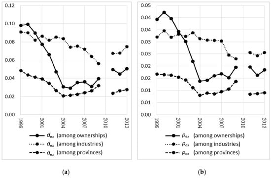
Figure 1.
Structual misallocation degree of dual factors. (a) Absolute misallocation degree of dual factors from 1998 to 2013; (b) relative misallocation degree of dual factors from 1998 to 2013. Notes: dex—absolute misallocation degree of dual factors; pex—relative misallocation degree of dual factors.
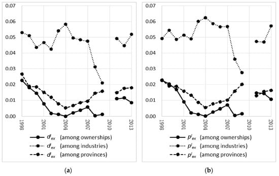
Figure 2.
Structual misallocation degree of labor. (a) Absolute misallocation degree of labor from 1998 to 2013; (b) relative misallocation degree of labor from 1998 to 2013. Notes: dlex—absolute misallocation degree of labor; plex—relative misallocation degree of labor.
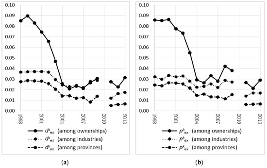
Figure 3.
Structual misallocation degree of capital. (a) Absolute misallocation degree of capital from 1998 to 2013; (b) relative misallocation degree of capital from 1998 to 2013. Notes: dkex—absolute misallocation degree of capital; pkex—relative misallocation degree of capital.
Figure 1a includes the absolute degree of different structural misallocations among ownership sectors, industries, and provinces. We can see that, by 2013, the absolute misallocation degree of factors among industries was the most serious, the absolute misallocation among ownerships ranked second, and the least degree of the misallocation was recorded among provinces. Figure 1b, which includes the relative misallocation degree, also shows the same rank of the three structural misallocations.
As to the trend of misallocation degree, from Figure 1a we can get that, with the deepening of China’s market-oriented reform, three types of structural misallocations have mitigated before 2008. The mitigation speed of misallocation among ownership sectors is the fastest from 1998 to 2004, while the misallocation degrees among ownerships and among provinces remained basically unchanged from 2004 to 2008. However, in order to resolve the world financial crisis, China increased the stimulus to aggregate demand after 2008, and the misallocations among ownership sectors and among industries became much more serious, and the misallocation among provinces increased slightly.
From Figure 2b, which shows the relative structural misallocation degree of labor, we can get that, the misallocation of labor among industries was most serious, followed by that among provinces, and that among ownership sectors was the least. From Figure 3b, which shows the relative structural misallocation degree of capital, we can get the misallocation degree of capital among ownership sectors was most serious, that among industries was second, and that among provinces was least.
Moreover, from Figure 2a, which shows the absolute distortion degree of labor, we can find that, the misallocation degree of labor among ownership sectors mitigated rapidly, but became much more serious after 2008. The misallocation among provinces also mitigated, but rebounded after 2004, especially after 2008. The misallocation among industries mitigated from 2004 to 2009, but rebounded very quickly after 2009. However, Figure 3a, which depicts the absolute misallocation degree of capital shows that, the three types of structural misallocation all mitigated before 2008, especially the misallocation among ownership sectors. But after 2008, the misallocation among ownership sectors rebounded slightly, while the misallocation among industries and provinces almost remain unchanged with fluctuation.
The financial crisis in the year of 2008 is an important dividing line. It made the three types of structural distortion of labor became more and more serious, especially to labor. To resolve the financial crisis, China invested much more on infrastructure and real estate, and provided much lower interest loans to state-owned firms to increase investment. Because of the manufacturing firms we use, the misallocation degree of capital among subindustries within manufacturing industry did not increase after financial crisis. However, the misallocation of capital among ownerships rebounded. Moreover, to resolve financial crisis, investment has been intensified in various regions, so the capital misallocation among regions did not increase. But after the financial crisis, unemployed migrant workers in the eastern regions went back to their hometowns, which were undeveloped, so the labor misallocation degree among regions increased.
6. Robustness
We calculated the misallocation degree with α as 0.45 in the above. Now, referring to Yang (2015), who recalculated α as 0.35 using OP method with industrial firms data, we recalculate the misallocation degree, as shown from Figure 4, Figure 5 and Figure 6. We can find that the results are in consistent with that in the above. Moreover, we also recalculate the degree using the data from 1998 to 2007 with α as 0.45, which includes the added value data and we can use it to measure the output of firms. The results are also in consistent with that in the above, which is shown in Appendix A.
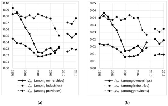
Figure 4.
Structual misallocation degree of dual factors. (a) Absolute misallocation degree of dual factors with α as 0.35; (b) relative misallocation degree of dual factors with α as 0.35. Notes: dex—absolute misallocation degree of dual factors; pex—relative misallocation degree of dual factors.
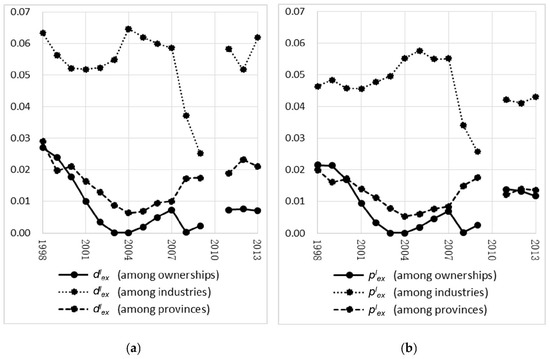
Figure 5.
Structual misallocation degree of labor. (a) Absolute misallocation degree of labor with α as 0.35; (b) relative misallocation degree of labor with α as 0.35. Notes: dlex—absolute misallocation degree of labor; plex—relative misallocation degree of labor.
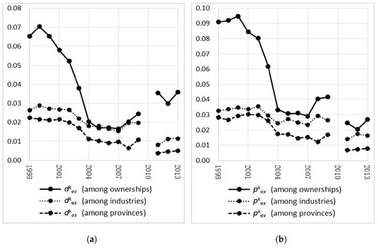
Figure 6.
Structual misallocation degree of capital. (a) Absolute misallocation degree of capital with α as 0.35; (b) relative misallocation degree of capital with α as 0.35. Notes: dkex—absolute misallocation degree of capital; pkex—relative misallocation degree of capital.
7. Conclusions
Structural reform will be very important for the sustainable development of China’s economy. But it is multifaceted, including the upgrade of industrial structure, the optimization of regional structure, the reform of ownership structure and so on. With this background and using the microdata of manufacturing firms in China from 1998 to 2013, we analyze the TFP loss caused by the misallocation of production factors among industries, among regions and among ownership sectors within the manufacturing industry.
We firstly propose a unified model that divides the whole economy into three layers: the state, the group, and the firm. With this model, we cannot only measure the absolute misallocation degree among groups, as per the BTZ model, but we can also measure the absolute misallocation degree among firms within groups, as per the HK model. As such, our model can measure the absolute total misallocation degree. Therefore, we can measure the relative misallocation degree using the ratio of the degree of single one structural misallocation to the degree of total misallocation. Then using the relative degree—not the absolute degree—to judge which structural misallocation is more serious will be more objective.
The measuring results show that: (1) The misallocation is very serious in China. It not only existed in the allocation of capital, but also in the allocation of labor. They almost caused the same national TFP loss, with an average of 97% and 91% respectively. (2) Compared with the misallocation among ownership sectors and provinces, the misallocation among industries was the most serious, which has led to the TFP loss of 7.7%. Meanwhile, we also find that the misallocation degree of labor among industries were higher than that of capital, and it was similar to the misallocation among regions. (3) When to analyze the misallocation degree of single production factor, it is found that the misallocation of capital among ownership sectors was the most serious, which has led to an annual TFP loss of around 5%. (4) A series of market-oriented reforms have achieved great results before 2008, and the structural misallocation has gradually eased, especially among the ownership sectors. However, after the financial crisis in 2008, with a series of policies to stimulate aggregate demand, the three types of structural misallocation have become worse, especially in labor.
Therefore, the policy implications are that: (1) It is need to continue to deepen structural reform, effectively shift the focus of policies to the supply side, and strive to promote China’s economic quality and TFP through optimizing the allocation of factors. While accelerating the development of capital market, we must also improve the labor market. (2) Further promoting the upgrade of the industrial structure is the priority for structural reform. (3) When to optimize the industrial structure, we should avoid excessive wage differentials among different industries and promote the free flow of labor forces across industries. When to optimize the regional structure, we should speed up the reform of household registration system, and realize the migrant workers settle down locally. (4) When to develop the capital market, we still need to pay more attention to the ownership discrimination in firm financing, and to construct a fairer environment for private firms.
Nevertheless, the present research also has some limitations. We mainly referred to the HK model to define the misallocation. If production factors flow from the firm or department with a low marginal product to the one with a high marginal product, the aggregate output would be higher. However, this is the only intensive misallocation defined by Banerjee and Moll [8], the more comprehensive misallocation also includes the distorted entrance and exit of firms, which is an extensive misallocation. In the future, we will try to introduce the entrance and exit process into our model [34,35,36,37] in order to analyze the structural misallocations more comprehensively. Beyond the direct loss of contemporaneous output, the dynamic loss led to by misallocation should be paid more attention [38]. In addition to analyzing the misallocation of production factors, we should still pay more attention to the misallocation of innovation resources [4,39] or land [40,41].
Author Contributions
Conceptualization, L.J. and C.M.; methodology, L.J. and C.M.; software, B.Z.; validation, L.J., C.M. and B.Z.; formal analysis, L.J. and C.M.; resources, B.Z.; data curation, B.Z. and B.Y.; Writing—original draft preparation, L.J.; Writing—review and editing, B.Z. and B.Y.; visualization, B.Y.; supervision, C.M. and B.Z.; funding acquisition, L.J.
Funding
This research was funded by National Natural Science Foundation of China and National Social Science Foundation of China, grant number 71803093 and 17ZDA114.
Acknowledgments
This paper is financially supported by National Natural Science Foundation of China (No. 71803093), China National Social Science Foundation of China (No. 17ZDA114), and K. C. Wong Magna Fund in Ningbo University. In addition, we thank the editors and the anonymous reviewers for their constructive comments and advice.
Conflicts of Interest
The authors declare no conflict of interest.
Appendix A

Figure A1.
Structual misallocation degree of dual factors. (a) Absolute misallocation degree of dual factors using added value data; (b) relative misallocation degree of dual factors using added value data. Notes: dex—absolute misallocation degree of dual factors; pex—relative misallocation degree of dual factors.

Figure A2.
Structural misallocation degree of labor. (a) Absolute misallocation degree of labor using added value data; (b) relative misallocation degree of labor using added value data. Notes: dlex—absolute misallocation degree of labor; plex—relative misallocation degree of labor.

Figure A3.
Structural misallocation degree of capital. (a) Absolute misallocation degree of capital using added value data; (b) relative misallocation degree of capital using added value data. Notes: dkex—absolute misallocation degree of capital; pkex—relative misallocation degree of capital.
References
- Solow, R.M. A contribution to the theory of economic growth. Q. J. Econ. 1956, 70, 65–94. [Google Scholar] [CrossRef]
- Gong, G. Contemporary Chinese Economy, 2nd ed.; High Education Press: Beijing, China, 2017. (In Chinese) [Google Scholar]
- Howell, A. Picking ‘winners’ in China: Do subsidies matter for indigenous innovation and firm productivity? Chin. Econ. Rev. 2017, 44, 154–165. [Google Scholar] [CrossRef]
- Wei, S.J.; Xie, Z.; Zhang, X. From “made in China” to “innovated in China”: Necessity, prospect, and challenges. J. Econ. Perspect. 2017, 31, 49–70. [Google Scholar] [CrossRef]
- Cai, F. How can Chinese economy achieve the transition toward total factor productivity growth? Soc. Sci. Chin. 2013, 1, 56–71. (In Chinese) [Google Scholar]
- Brandt, L.; Van Biesebroeck, J.; Zhang, Y. Creative accounting or creative destruction? Firm-level productivity growth in Chinese manufacturing. J. Dev. Econ. 2012, 97, 339–351. [Google Scholar] [CrossRef]
- Restuccia, D.; Rogerson, R. Policy distortions and aggregate productivity with heterogeneous establishments. Rev. Econ. Dyn. 2008, 11, 707–720. [Google Scholar] [CrossRef]
- Banerjee, A.V.; Moll, B. Why does misallocation persist? Am. Econ. J. Macroecon. 2010, 2, 189–206. [Google Scholar] [CrossRef]
- Hsieh, C.T.; Klenow, P.J. Misallocation and Manufacturing TFP in China and India. Q. J. Econ. 2009, 124, 1403–1448. [Google Scholar] [CrossRef]
- Brandt, L.; Tombe, T.; Zhu, X. Factor market distortions across time, space and sectors in China. Rev. Econ. Dyn. 2013, 16, 39–58. [Google Scholar] [CrossRef]
- Yang, R. Study on the total factor productivity of Chinese manufacturing enterprises. Econ. Res. J. 2015, 2, 61–74. (In Chinese) [Google Scholar]
- Bin, P.; Chen, X.; Fracasso, A.; Tomasi, C. Resource allocation and productivity across provinces in China. Int. Rev. Econ. Financ. 2018. [Google Scholar] [CrossRef]
- Shao, Y.; Bu, X.; Zhang, T. Resource misallocation and TFP of Chinese industiral enterprises—A recalculation based on Chinese industrial enterprises database. Chin. Ind. Econ. 2013, 12, 39–51. (In Chinese) [Google Scholar] [CrossRef]
- Chen, S.; Jefferson, G.H.; Zhang, J. Structural change, productivity growth and industrial transformation in China. Chin. Econ. Rev. 2011, 22, 133–150. [Google Scholar] [CrossRef]
- Mallick, J. Structural Change and Productivity Growth in India and the People’s Republic of China. In ADBI Working Papers; No. 656; 2017; Available online: https://www.adb.org/sites/default/files/publication/226566/adbi-wp656.pdf (accessed on 5 November 2018).
- Aoki, S. Was the Barrier to Labor Mobility an Important Factor for the Prewar Japanese Stagnation? In MPRA Working Paper; No. 8178; 2008; Available online: http://mpra.ub.uni-muenchen.de/8178/ (accessed on 5 November 2018).
- Aoki, S. A simple accounting framework for the effect of resource misallocation on aggregate productivity. J. Jpn. Int. Econ. 2012, 26, 473–494. [Google Scholar] [CrossRef]
- Restuccia, D.; Rogerson, R. Misallocation and productivity. Rev. Econ. Dyn. 2013, 16, 10–21. [Google Scholar] [CrossRef]
- Hopenhayn, H.A. Firms, misallocation, and aggregate productivity: A review. Annu. Rev. Econ. 2014, 6, 735–770. [Google Scholar] [CrossRef]
- Yuan, Z.; Xie, D. The effect of labor misallocation on TFP: China’s evidence 1978–2007. Econ. Res. J. 2011, 7, 4–17. (In Chinese) [Google Scholar]
- Chen, Y.; Hu, W. Distortions, misallocation and losses: Theory and application. Chin. Econ. Q. 2011, 10, 1401–1422. (In Chinese) [Google Scholar] [CrossRef]
- Han, J.; Zheng, Q. How does government intervention lead to regional resource misallocation—Based on decomposition of misallocation within and between industries. Chin. Ind. Econ. 2014, 11, 69–81. (In Chinese) [Google Scholar] [CrossRef]
- Jin, L.; Lin, J.; Ding, S. Effect of administrative monopoly on resources misallocation caused by ownership differences. Chin. Ind. Econ. 2015, 4, 31–43. (In Chinese) [Google Scholar] [CrossRef]
- Chen, S. Misallocation, economic growth performance and the market entry of firms: A dual perspective of state and non-state sectors. AC. Mon. 2017, 1, 42–56. (In Chinese) [Google Scholar]
- Zhang, T.; Zhang, S. Biased policy, resource allocation and aggregate productivity. Econ. Res. J. 2016, 2, 126–139. (In Chinese) [Google Scholar]
- Lu, X.; Lian, Y. Estimation of total factor productivity of industrial enterprises in China: 1999–2007. Chin. Econ. Q. 2012, 11, 541–558. (In Chinese) [Google Scholar] [CrossRef]
- Brandt, L.; Zhu, X. Accounting for China’s Growth. In IZA Discussion Paper; No. 4764; 2010; Available online: https://ssrn.com/abstract=1556552 (accessed on 5 November 2018).
- Olley, G.S.; Pakes, A. The dynamics of productivity in the telecommunications equipment industry. Econometrica 1996, 64, 1263–1297. [Google Scholar] [CrossRef]
- Foster, L.; Haltiwanger, J.; Syverson, C. Reallocation, firm turnover, and efficiency: Selection on productivity or profitability? Am. Econ. Rev. 2008, 98, 394–425. [Google Scholar] [CrossRef]
- Levinsohn, J.; Petrin, A. Estimating production functions using inputs to control for unobservables. Rev. Econ. Stud. 2003, 70, 317–341. [Google Scholar] [CrossRef]
- Ackerberg, D.A.; Caves, K.; Frazer, G. Identification properties of recent production function estimators. Econometrica 2015, 83, 2411–2451. [Google Scholar] [CrossRef]
- Song, Z.; Storesletten, K.; Zilibotti, F. Growing like China. Am. Econ. Rev. 2011, 101, 196–233. [Google Scholar] [CrossRef]
- Hsieh, C.T.; Song, Z. Grasp the Large, Let Go of the Small: The Transformation of the State Sector in China. In NBER Working Papers; No. w21006; 2015; Available online: http://www.nber.org/papers/w21006 (accessed on 5 November 2018).
- Bartelsman, E.; Haltiwanger, J.; Scarpetta, S. Cross-country differences in productivity: The role of allocation and selection. Am. Econ. Rev. 2013, 103, 305–334. [Google Scholar] [CrossRef]
- Peters, M. Heterogeneous Mark-Ups, Growth and Endogenous Misallocation. In LSE Working Paper; No. 54254; 2013; Available online: http://eprints.lse.ac.uk/54254/ (accessed on 5 November 2018).
- Midrigan, V.; Xu, D.Y. Finance and misallocation: Evidence from plant-level data. Am. Econ. Rev. 2014, 104, 422–458. [Google Scholar] [CrossRef]
- Moll, B. Productivity losses from financial frictions: Can self-financing undo capital misallocation. Am. Econ. Rev. 2014, 104, 3186–3221. [Google Scholar] [CrossRef]
- Restuccia, D.; Rogerson, R. The causes and costs of misallocation. J. Econ. Perspect. 2017, 31, 151–174. [Google Scholar] [CrossRef]
- Li, H.C.; Lee, W.C.; Ko, B.T. What determines misallocation in innovation? A study of regional innovation in China. J. Macroecon. 2017, 52, 221–237. [Google Scholar] [CrossRef]
- Huang, Z.; Du, X. Government intervention and land misallocation: Evidence from China. Cities 2017, 60, 323–332. [Google Scholar] [CrossRef]
- Restuccia, D.; Santaeulàliallopis, R. Land Misallocation and Productivity. In NBER Working Papers; No. w23128; 2017; Available online: http://www.nber.org/papers/w23128 (accessed on 5 November 2018).
© 2018 by the authors. Licensee MDPI, Basel, Switzerland. This article is an open access article distributed under the terms and conditions of the Creative Commons Attribution (CC BY) license (http://creativecommons.org/licenses/by/4.0/).