Abstract
Not all urban low-voltage grids will be able to integrate new loads such as charging infrastructure for electric mobility or electrical heat pumps into existing structures without further measures. Therefore, this article analyzes to what extent load management is more cost-effective than conventional grid expansion. Methodically, the different load types are first apportioned from country to grid-level on the basis of different parameters. Subsequently, both conventional grid planning as a reference variant and innovative grid planning with different variants of load management are carried out. As a result, it can be summarized that the future success of load management is strongly dependent on its costs and whether the necessary information and communication technology is already deployed in the grids. Regardless of the costs, there is also considerable potential for savings in conventional grid expansions.
1. Introduction
In the event that more and more charging infrastructure for electric vehicles (EVs), be it private (PrCPs) or public charging points (PuCPs), is continuously integrated into urban distribution grids, it must be ensured that these low-voltage (LV) grids are dimensioned accordingly. The progressive electrification of the heating sector, for instance with electrical heat pumps (HPs), must also be taken into account. Depending on the existing load and the available capacity, the grids cannot integrate new loads to a significant extent. Therefore, conventional grid expansion measures or innovative technologies in the form of load management, for example, which takes into account PrCPs, PuCPs, and HPs in various combinations, are required to ensure that technical planning limits concerning voltage and loading are observed.
1.1. Literature Review and Novelty
So far, the focus in many studies has been on PrCPs without simultaneous consideration of PuCPs with a higher power than 22 kW in LV grids, as is the case in [1,2,3,4,5] for example. In addition, there are few studies, such as [6,7], that consider load management, but not yet with such an extensive evaluation of different combinations of PrCPs, PuCPs, and HPs and their effects on grid planning. Furthermore, in [7], among other assumptions, it is assumed that 22 kW charging points (CPs) are reduced to a minimum of 11 kW instead of 3.7 kW as is the case in this article.
1.2. Structure and Objective
Firstly, this article lists various scenarios of electric mobility and HPs, two of which are selected for each mentioned load type in order to establish a corridor as an upper and a lower load development band. This is followed by a detailed description of the method to apportion scenario values of load development, which considers the two load types CPs and HPs. In order to interpret the results accordingly, the general conditions are then presented for both the selected operating points and two planning perspectives, as well as the limit values and power value assumptions to be observed. This is followed by a description of the conventional planning measures and the load management, as an innovative planning measure, that is modeled.
At the end of the article, the planning measures are evaluated to subsequently classify and discuss the results. Initially, the respective measures are explained without corresponding costs for the planning perspectives. This is followed by an evaluation of the costs for different variants of the load management with different equipment and of the saving potential by comparing the different approaches.
The basic objective of this article is, therefore, to present new methods for grid planning, to apply them in a large-scale planning study, and to evaluate dynamic load management (DLM) in three variants for urban LV grids.
2. New Loads in Urban Low-Voltage Grids
In grid planning, a fundamental distinction must be made between decentralized energy generation, such as photovoltaic systems, which are increasingly found in rural grids, and new loads such as CPs and HPs in urban grids, whereas the latter are increasingly found in suburban grids. Even though the focus here is on urban grids, decentralized energy generation cannot be completely excluded in principle, but it can be expected that the influence of new loads outweighs decentralized generation considerably.
By aiming for region-specific investigations along with the consideration of sustainable and efficient grid planning, it is necessary to consider the development of new loads, in particular CPs and HPs. Different development trends will have different impacts on determining their expected distribution in cities, municipalities, and districts. In order to achieve an accurate investigation and a fundamental framework for future grid planning done by distribution system operators (DSO), these projections need to be based on sufficiently precise assumptions. The main objective here is the appropriate planning of distribution grids so that they can be operated efficiently and cost-optimally to meet the upcoming integration of a large number of new loads. To take the uncertainty in load development into account, scenario analysis is used. The upcoming part describes the developed methodology for the distribution of those mentioned new loads down to grid level. It starts with the input data used in the apportionment and finally the resulting apportionment methodology.
2.1. Scenarios
The initial data, the basis for the scenarios of the new loads, stem from studies that specify EV and HP penetration in a certain country. The studies project the penetration based on several assumptions, such as governmental plans, the existing state of mobility or heating sector, and/or the state of technology. Here, scenarios of Germany are considered as input data for the methodology. The scenarios have been interpolated and extrapolated to model the development trajectory of the penetration of new loads in five-year intervals from 2020 to 2050. The ten-year intervals from 2020 to 2050 represent the benchmark years considered in this article.
The extrapolated development trajectories can then be compared to one another to perform an analysis of the different benchmark years. The trajectory of the penetration of new loads at each benchmark year is used to map possible realistic development paths or outline corridors in the context of grid planning. Not to be overlooked is the fact that the scenario values are still prognoses based on assumptions. Uncertainties depending on a clear development of the present mobility or heating sector trend as well as significant amendments of technical, economic, and regulatory conditions, can be accurate only to a limited extent. However, these uncertainties can be translated into a tolerance band, which is taken into account in the planning of the power grids and helps to gain knowledge about the influence of different input parameters on the respective grids.
2.1.1. Electric Mobility
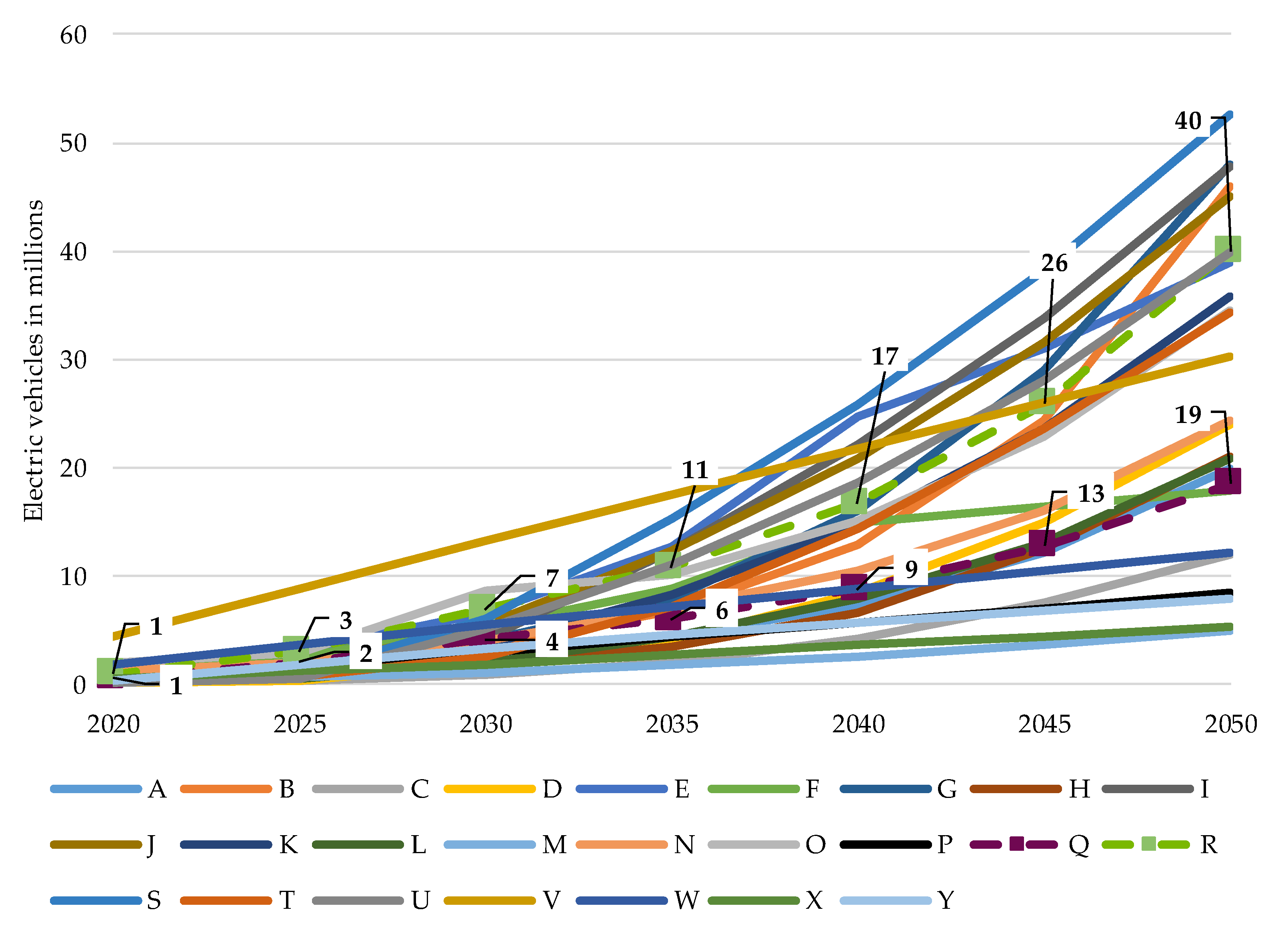
Figure 1 and Table 1 show various scenarios for the development of electric mobility in Germany. Older studies are grayed out. Apart from the fact that the individual studies are based on different assumptions, the two scenarios Q and R are selected from a relatively recent study [8], which divides the range into three equal corridors.
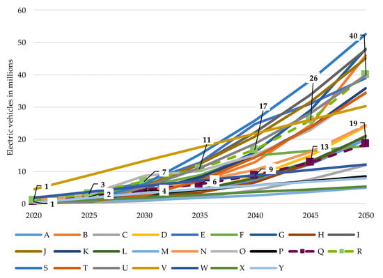
Figure 1.
Development trajectories for electric vehicle development scenarios in Germany.

Table 1.
Researched scenarios for the development of electric vehicles.
2.1.2. Power-to-Heat
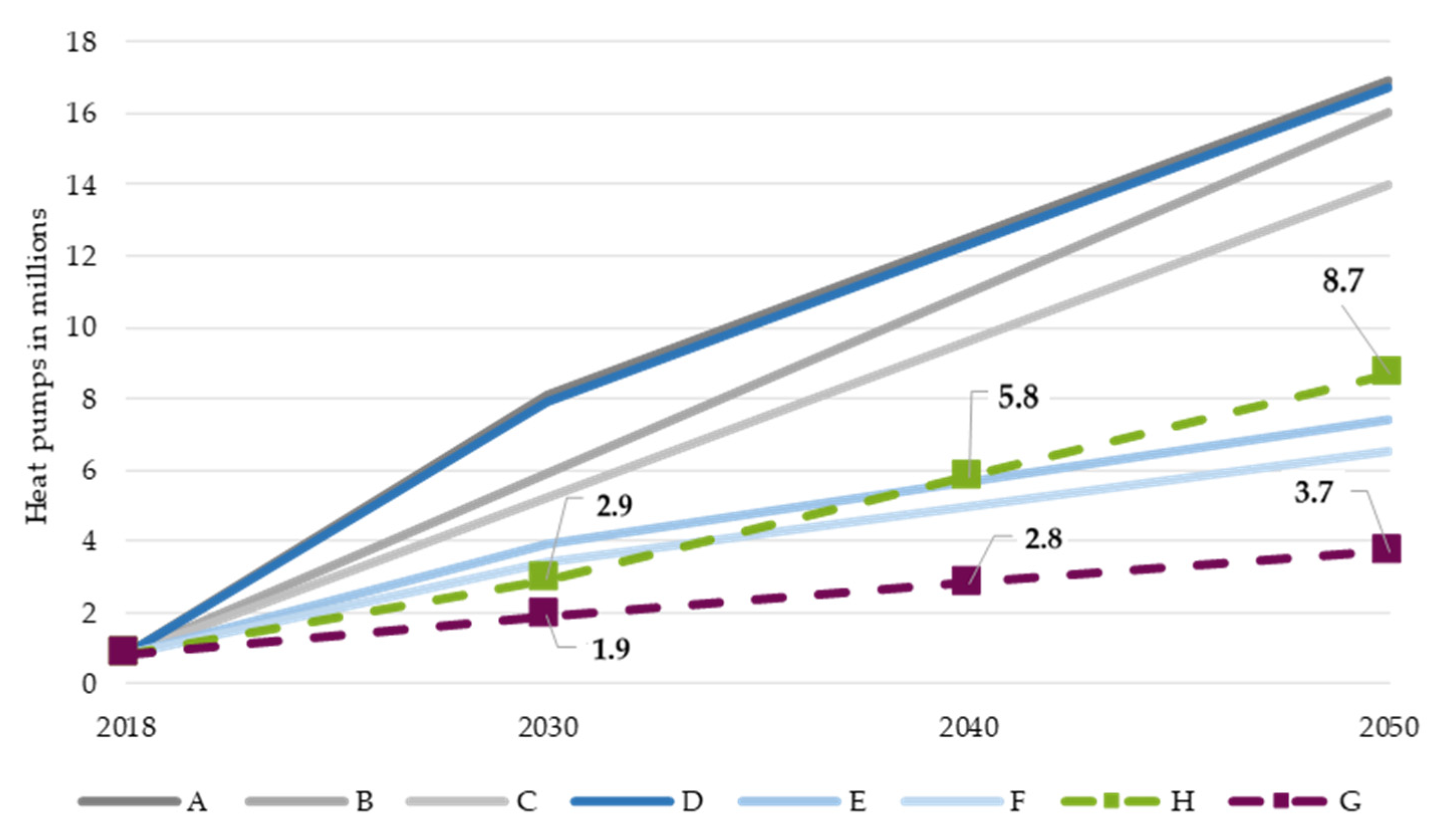
Figure 2 and Table 2 depict trajectories that represent the possible scenarios for HPs in Germany. For example, on the one hand, scenarios A to F outline paths to achieve the climate goals. On the other hand, scenarios G and H assume a current market development as well as already set or firmly planned framework conditions to support the heating market. Therefore, scenarios G and H are chosen for apportionment.
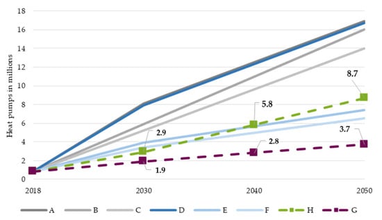
Figure 2.
Ramp-up trajectories of heat pump development scenarios for Germany based on [20], own representation.
Table 2.
Studies used as a basis for the development of heat pumps.
2.2. Apportionment Methodology
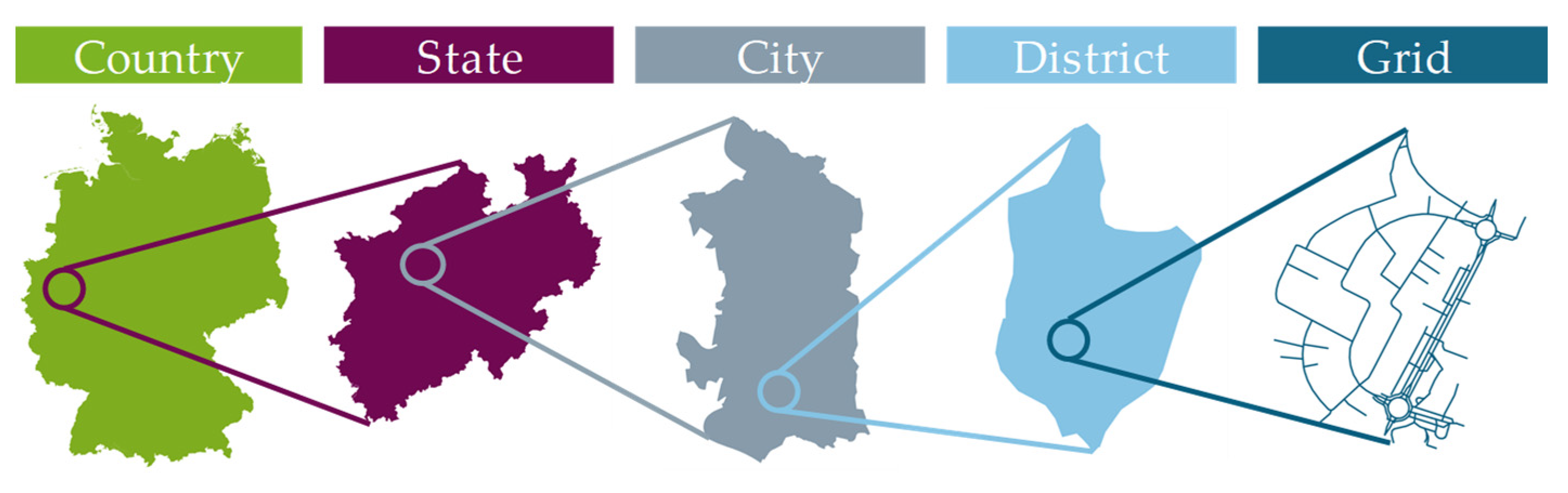
Figure 3 illustrates the implemented approach of the apportionment methodology in five steps. The first step identifies the scenarios at a country level, namely Germany, for the status quo and the selected benchmark years 2030, 2040, and 2050. In the second step, the scenarios are broken down at the state level. The last three steps provide a more in-depth allocation at the city, the district, and the grid level. The apportionment methodology described below can be used for EVs or CPs and HPs when taking into account the appropriate parameters.

Figure 3.
Steps of the regionalization methodology.
2.2.1. Charging Infrastructure on City Level
The allocation of EVs is available at the country level in Germany. To determine values at the state level (S), the country values are multiplied with several distribution factors that differentiate the states from each other. Each of the distribution factors is then multiplied with a weighting term, where the sum of the weighting terms equals one. The weighting terms express the impact of the single distribution factor on the total number of EVs in a certain state. In this apportionment methodology, six distribution factors (F) are determined. Each is expressed with a weighting term (a, b, c, d, e, and f) [24]. The distribution factors considered are the current population of the state (POP), the number of EVs in the state (EV), the number of car owners in the state (CO), scientific research budget for electric mobility (RB), number of buildings (B), and total vehicles registered in the state (V). All of these factors are calculated in relation to the respective data on the country level. Equation (1) shows the combination of the distribution factors at the state level [24].
To get the values on the municipality (MU) level, the state values are multiplied with three different distribution factors. Each is in combination with a weighting term (k, l, and m) [24]. The considered distribution factors on the MU level are population (POP), population density (POPD), and total vehicles registered (V) per municipality. Equation (2) shows the derived formula to calculate the number of EVs at the MU level [24].
2.2.2. Electrical Heat Pumps on City Level
The distribution of HPs at the state level is carried out similar to EVs. Hence, the apportionment of the country wide scenario values at the state level is performed proportionally to the existing number of HPs. It is assumed that the relative allocation of HPs remains constant among the states. After calculating scenario values at the state level, the subsequent step is to scale down the number of HPs further to the respective cities and municipalities [25].
The capability of HPs in supplying the thermal heat demand in proportion to the required electric power is then analyzed. Furthermore, the feasibility of HPs in different building types is investigated. From there, it is assumed that HPs are mainly installed in detached or semi-detached buildings. These data are available under [26] for each city and municipality in Germany. In the apportionment methodology, this specific data is associated with the state in order to define the allocation for each examined city or municipality. The number of HPs per state is afterwards scaled down according to the building database onto the city and municipality level [25].
In order to distribute the present number of HPs for a city or municipality to the respective districts, it is advisable to use data of the respective DSO. Since detached buildings or semi-detached buildings with one or two apartments normally have less than or equal to two metering points per address, these metering points are filtered in order to locate them. This procedure is also employed within a city to distribute the HPs on such buildings, which as an example have a bakery on the ground floor and a residential apartment on the second floor. The number of HPs then calculated per district is associated with the entire city. So, that in addition to cities, also each district has its own distribution key. Alternatively, the building structure data can also be used (e.g., data on (semi-)detached buildings) [25].
2.2.3. Distribution on Grid Level
Finally, the methodology of the allocation to the respective districts, and subsequently the distribution on street level, is similar for both EVs and HPs (see Figure 4). First, the unit numbers of general EVs are categorized as residential, commercial, and commuter based on building data. Residential (RB) and mixed-use (MB) buildings (both commercial (CB) and residential) are related to private EVs. For commercial EVs, all building types are used, and for commuters, only MBs and CBs are used. The only difference to HPs is the considered building types. For private EVs, the incorporated buildings parameter considers all residential buildings in comparison to the parameter “detached (DB) and semi-detached (SB) buildings” for HPs. The reason is that EVs can be found in any type of residential building, whereas HPs are—presumably—only to be installed in detached and semi-detached buildings. This is also due to the fact that HPs can be better integrated into detached and semi-detached buildings rather than in apartment buildings [25].
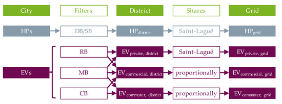
Figure 4.
Approach to allocating new loads from city to grid level.
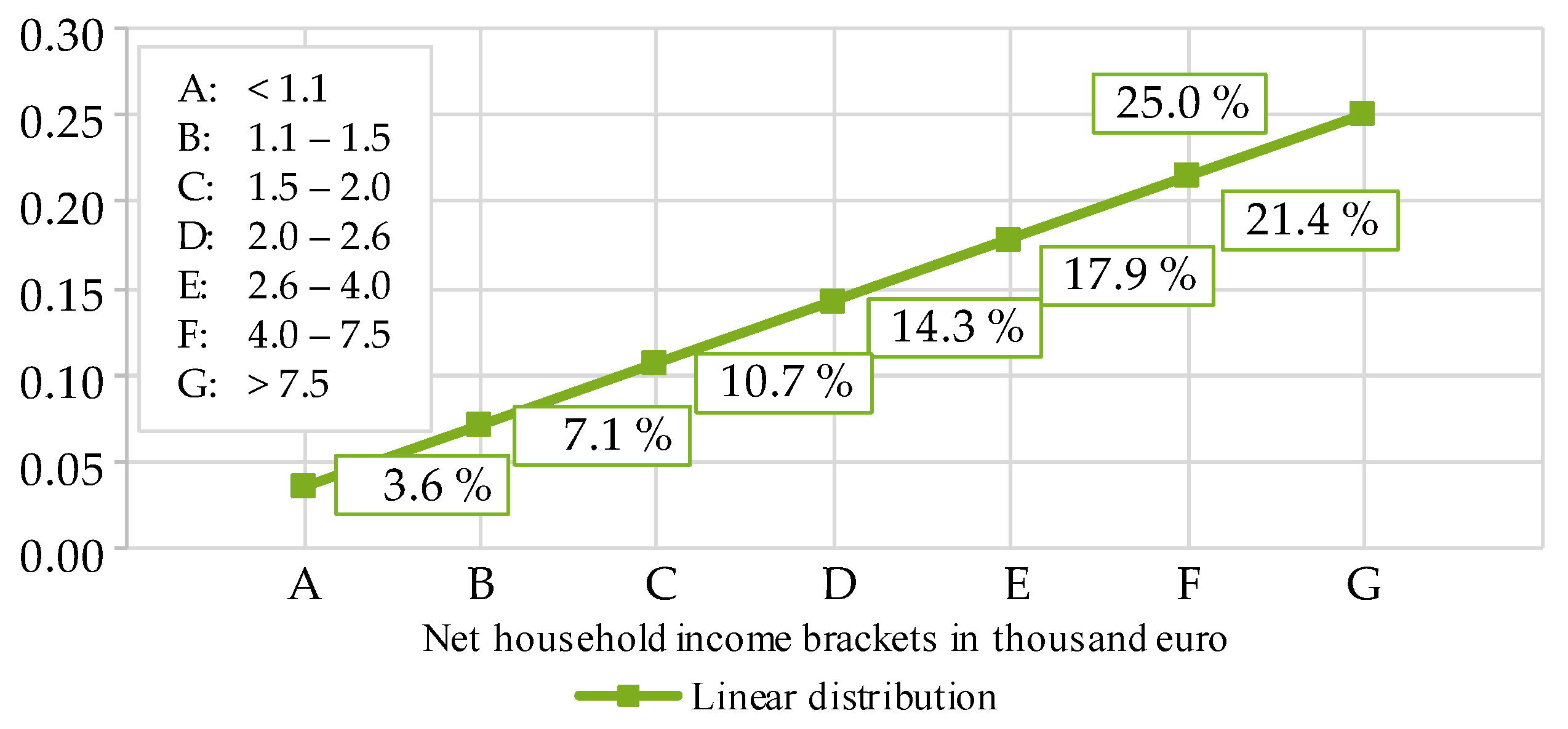
The last level of the apportionment methodology, and also the highest achievable resolution of the described method, is the distribution at the grid or street level. To achieve this, commercial socio-economic data [27] are utilized for private EVs and HPs. The market data are available as “population structure data” on street level with geo coordinates. In the first step, a linear distribution of the household net income on a street level is assumed within the districts, as shown in Figure 5. The result of this linear distribution is then used to determine the distribution factors for each building in this district. In the second step, by feeding the distribution factors into the iterative Saint-Laguë technique [28] (divisor method with standard deviation), the distribution on street level is accomplished [25].
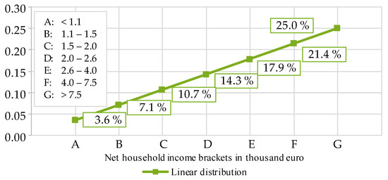
Figure 5.
A linear distribution of the net household income brackets A to G (sums up to 100%).
Since it can be assumed that, in contrast to private EVs and HPs, net household income will not have a major influence on commercial EVs and commuters, these numbers of EVs are apportioned from the local district to the grid level only based on the proportional building structures in the respective grid area (see Figure 4).
2.2.4. Charging Points and Heat Pumps within the Grids
After the apportionment method has determined the numbers of EVs and HPs at the grid level, these still have to be distributed within the grids to be able to take them into account in a power-flow calculation. For this purpose, the number of PrCPs is derived directly from the number of private and commercial EVs. For PuCPs, the total number of EVs in the LV grid is aggregated and multiplied by a factor of 1/13 according to [8]. Based on the underlying grid data, the CPs and HPs are iteratively distributed in the grid. HPs are integrated primarily at detached buildings, which have one metering point per house connection. PrCPs are distributed in such a way that one CP is distributed to detached buildings, two CPs to semi-detached buildings (two metering points per house connection), and also on average two CPs to multifamily buildings (load node as building connection). Underground garages for apartment buildings are not taken into account since there are no underground garages at apartment buildings in the analyzed LV grids. However, for other LV grids, underground garages are mandatory to be considered in individual cases if they are present. In general, a maximum of one PuCP is placed per grid node (e.g., cable distribution cabinet).
3. General Conditions
In the following, the general assumptions for the planning approach are described.
3.1. Power Value Assumptions
The new loads described in Section 2 must be provided with power values to determine the grid state. Therefore, the load at each node is required. Here, PSS©SINCAL Version 15.5 is used for the calculations.
In the field of electric mobility, corresponding power assumptions can be taken from Table 3, whose distributions of charging powers change over the benchmark years (assumed constant from 2040) [29].
Table 3.
Assumptions on distribution for private and public charging points over the benchmark years.
For HPs, three power value assumptions (3.0 kW, 6.5 kW, and 9.0 kW) are made that do not change over the years [30]. In summary, these three HP-Variants are calculated for two scenarios in which the distribution of the CP power always remains the same. This results in a total of six analyses, each with three benchmark years per LV grid (e.g., 3.0 kW HPs in the progressive scenario as upper load band for the year 2040 or 9.0 kW HPs in the conservative scenario as lower load band for the year 2050). With 14 LV grids analyzed, this results in 252 grid planning variants per planning technology.
3.2. Operating Points
There are two operating points of the grid, which are relevant for planning and dimensioning LV grids. These two operating points do not necessarily have to be real conceivable operating points but rather have to ensure the correct dimensioning of grid equipment.
On the one hand, there is the operating point “peak generation”, which, as already briefly explained in Section 2, is not considered in the further analysis. This is due to the significantly lower share of, e.g., photovoltaic systems compared to new loads in urban LV grids. Instead, only the operating point “peak load” is used as a basis, in which all distributed generation is neglected so that only loads remain in the grids, which assumes that the consumers cause the maximum simultaneous power demand.
3.3. Planning Perspectives and Simultaneity Factors
In the previous section, the term simultaneity was already mentioned, which is an elementary component of grid planning. In principle, grid equipment is not designed in such a way that the maximum possible load must be supplied in a grid, because it can be assumed that not all loads are operated in the grid at the same time. Therefore, so-called simultaneity factors (SFs) are taken into account. The SF is, thus, the ratio of the maximum simultaneous total demand to the sum of the maximum individual power demands.
3.3.1. Calculation of Simultaneity Factors for Charging Points
Four different calculation (C1 to C4) approaches to determine the simultaneity for charging infrastructure can be formulated as Equations (3)–(6).
with:
- i = charging power type
- PCPi = charging power per charging point type
- Pi = charging power per type
- nCPi = number of charging points per charging power
- ∑nCP = number of all charging points
- PØ = average charging power based on the distribution in the respective grid
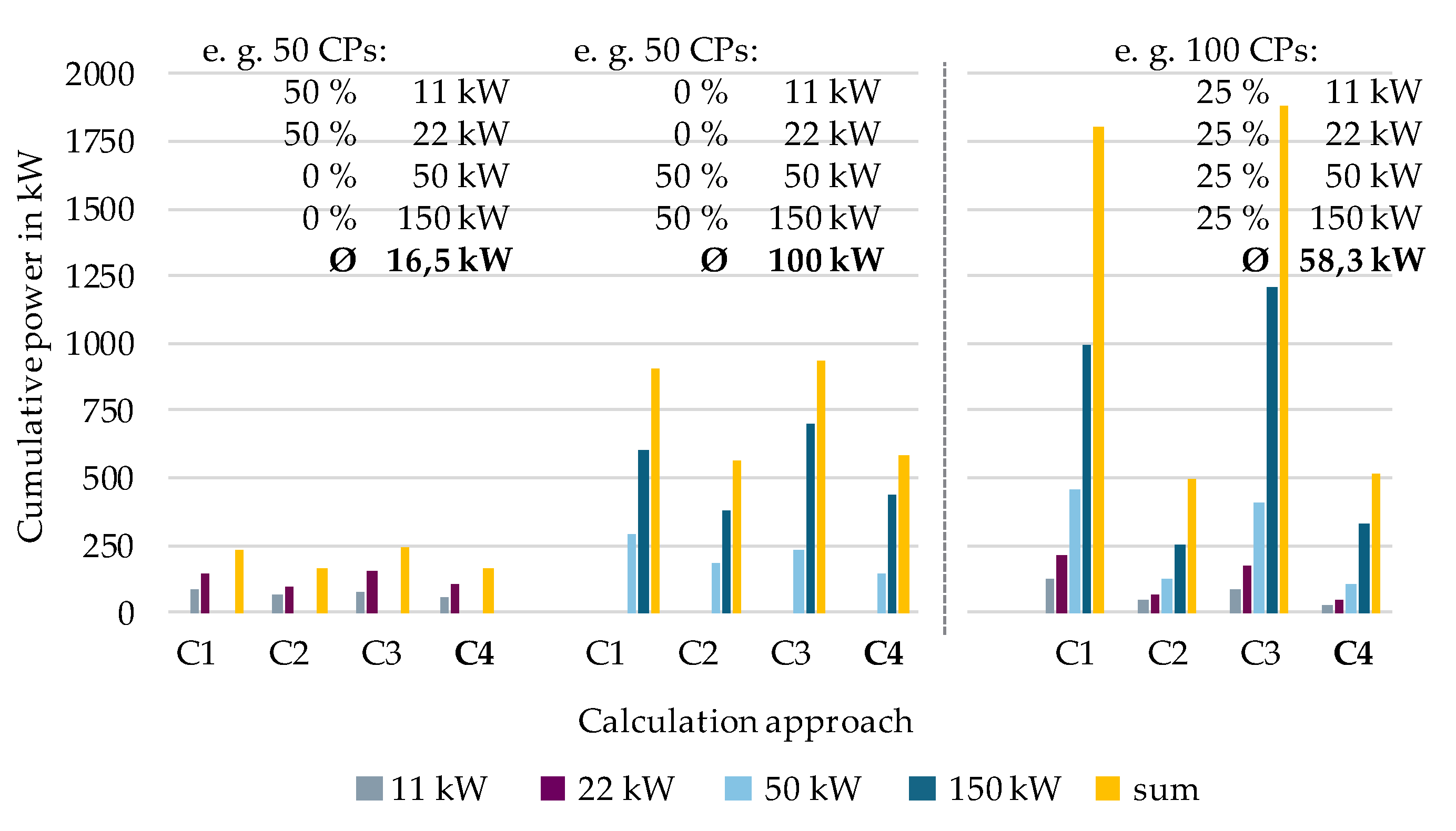
Calculation C1 describes the multiplication of the respective charging power with the SF for the respective charging power for the number of CPs for this charging power. C2 uses the number of all CPs in the grid instead. In contrast to C1 and C2, C3 and C4 do not use the respective charging power, but the average charging power in the grid. A comparison of these calculations can be found in Table 4. It can be seen directly that C4 uses only one SF per grid. However, to be able to estimate which differences result from the calculations regarding the cumulative power in the grid, an example can be taken from Figure 6. The left group of bars shows PrCPs, the middle group PuCPs and the right group a combination of both. It can be seen that C1 and C3 as well as C2 and C4 are very similar. Furthermore, it can be seen that C1 and C3 are significantly higher than the C2 and C4 and are estimated to be too high with 100 CPs with a cumulative of approximately 1.8 MW compared to approximately 500 kW in C2 and C4.
Table 4.
Comparison of different simultaneity factor calculations for charging infrastructure.
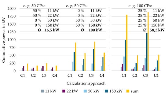
Figure 6.
Example of cumulative charging capacities with a different calculation of simultaneities for charging points (CPs).
From the previously presented evaluation of the calculation of simultaneity for charging infrastructure, the calculation method C4 will be used for all further analyses in the following.
3.3.2. Planning Perspectives for the Dimensioning of the Distribution Transformer and Outgoing Feeders under Consideration of Simultaneity Factors
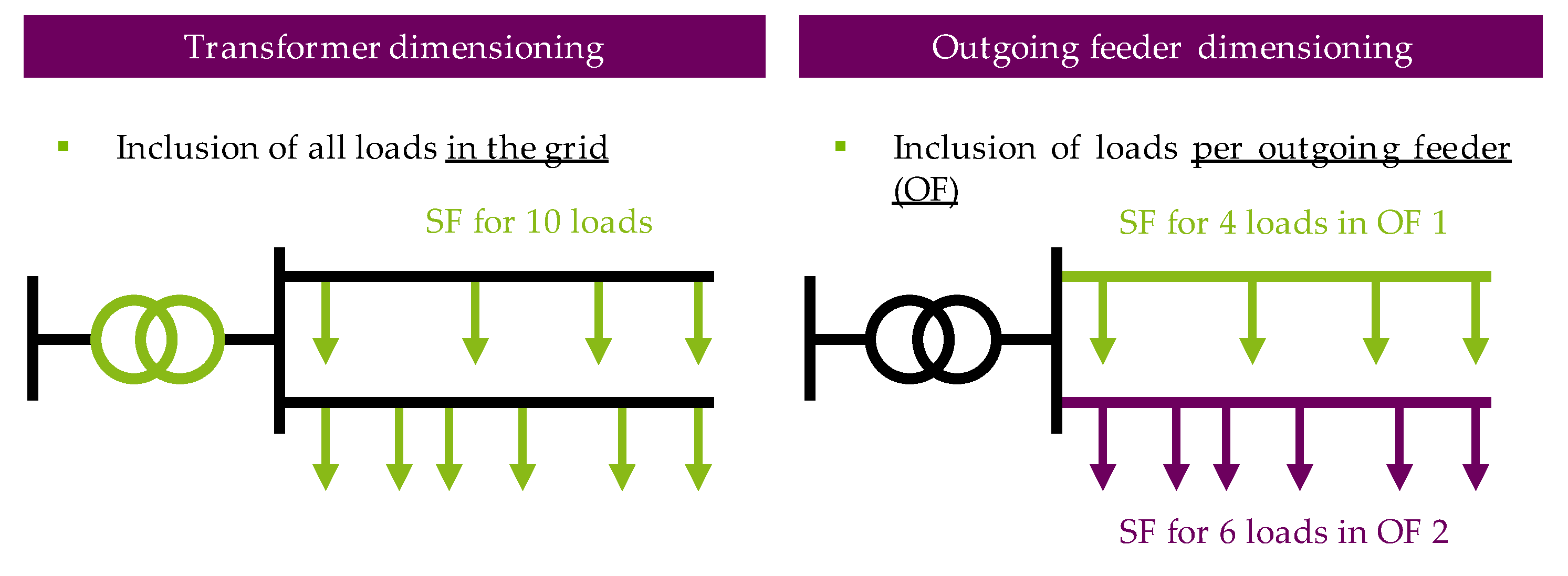
In combination with Section 3.2, Section 3.3, and Section 3.3.1, the following section explains how different grid equipment is dimensioned in the grid calculation software. Figure 7 shows the two procedures. On the left as well as on the right, an exemplary grid is shown, in which a distribution transformer (DT) supplies two outgoing feeders (OFs) with a different number of loads in each. The SF depends on the number of loads that must be supplied at the same time. When dimensioning the DT all connected loads in the grid must be taken into account. If a single OF is dimensioned, the number of connected loads is lower, which results in a higher SF. Using the same factors applied for the dimensioning of the OF would overestimate the required transformer capacity. This neglects the fact that this calculation must be performed per line section. This results in oversized line sections in some places, which only have to supply a small number of loads. In practice, however, it is common practice in many cases to use a standard cable cross-section for lines regardless of the exact number of directly connected loads.
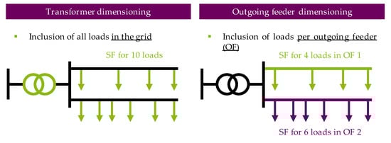
Figure 7.
Planning perspectives taking into account the respective simultaneity factor (SF).
3.4. Limit Violations for Grid Planning
After the LV grids have been modeled for the scenarios, HP-Variants and benchmark years in the grid calculation software, limits must be specified in order to be able to identify limit value violations during grid planning and to eliminate them with suitable planning measures.
According to [31], with respect to the voltage band, it is specified that ±10% of the nominal voltage must be observed. The voltage at the low-voltage side of the DT (slack) is set to 95% in the modeled grids, which represents the voltage at the secondary side. So, a voltage drop of a maximum of 5% is still allowed within the LV grids. As soon as this value is exceeded, regardless of the year, planning measures must be taken to remedy this limit violation.
In addition to exceeding the voltage limit, thermal equipment overloads can also occur both from the perspective of the DT as well as from the perspective of the respective line (not only OF). Irrespective of the fact that in practice an overload of 120% is also temporarily accepted, for example to the DT and the power lines in the event of a fault, the loading is limited to 100% of the rated value.
4. Load Management Systems
A load management in this article is defined as a system that adjusts the active power of selected loads depending on the current grid state as a DLM for different variants.
4.1. Variants of Dynamic Load Management and Usability
Table 5 shows three different variants of a DLM that control different loads [30]. The power output of the respective CPs is limited to a maximum of 3.7 kW. Thus, no selective switching off is considered in order to analyze which (base) loads are to be expected in the grids, unless specific switching off of the CPs is possible [30].
Table 5.
Control of the loads within the DLM-Variants.
For HPs, a switch-off is considered by adopting so-called turn-off periods. In DLM-Variant 1, HPs are switched off before the charging infrastructure is, because HPs can rely on heat storage as a back up when turn-off periods exist, so that the end-customer does not initially experience any loss of comfort. However, it must be explicitly pointed out that HPs are switched on again after a turn-off period is over. So, this DLM-Variant 1 is only intended to show what is possible in principle with intelligent control, without claiming it to be realistic. DLM-Variant 3 is also classified as rather theoretical [30].
4.2. Modeling Process for Distribution Transformers and Outgoing Feeders
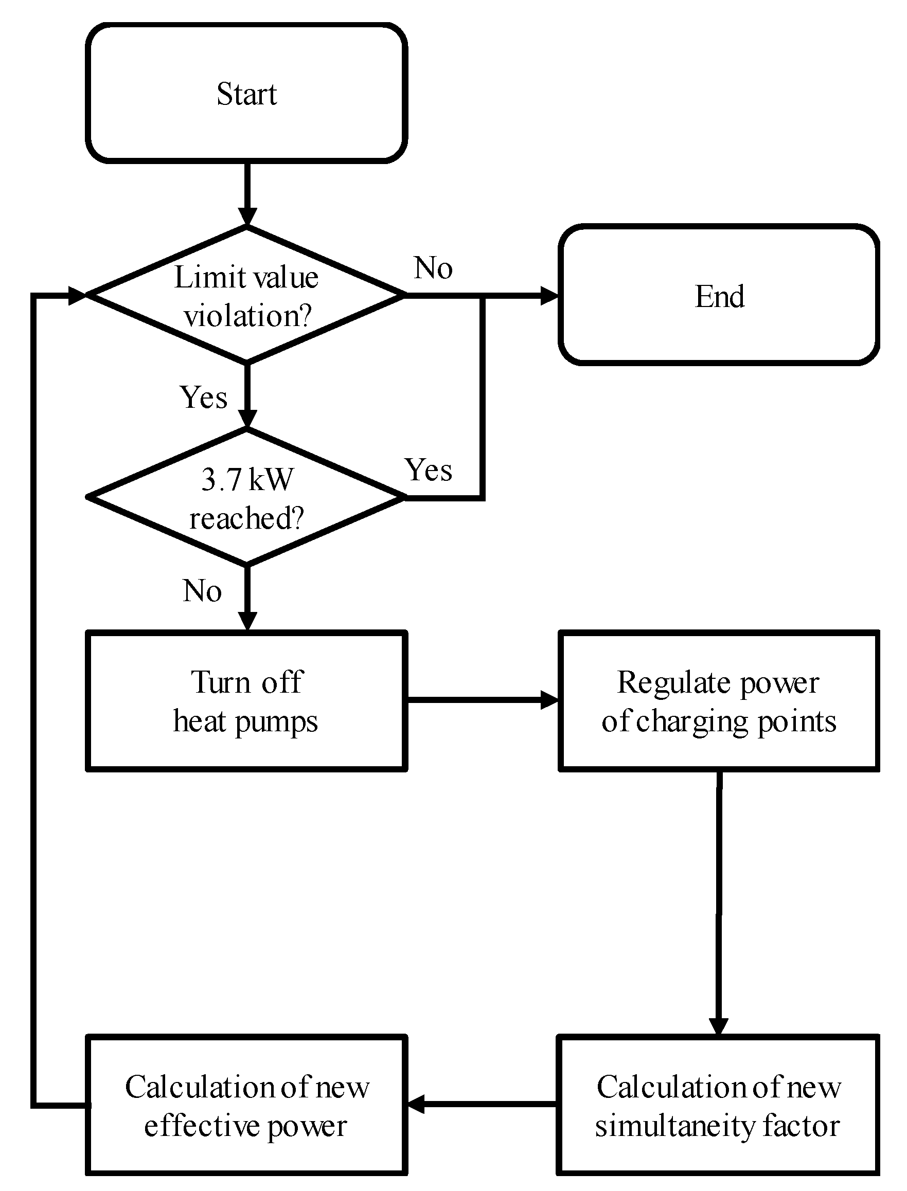
In Figure 8 and Figure 9, the simplified process flows can be seen from the perspective of DTs and OFs. Both processes are similar. The difference is that from the perspective of the OFs, each individual OF is analyzed with a power-flow calculation, whereas this is not necessary from the perspective of the DTs, since they consider all loads in the respective grids [30].

Figure 8.
Process flow for the distribution transformers under consideration of heat pumps [30].
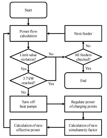
Figure 9.
Process flow for the outgoing feeders under consideration of heat pumps [30].
Therefore, the first step is to check whether equipment overloads (DT and OF) or violation of the lower voltage limits (only OF) occur. As soon as this is the case, all HPs (per OF or all for DTs) are switched off first in DLM-Variant 1. If there are still limit violations, the controlled CPs are reduced in 1-kW-steps to a maximum of 3.7 kW until limit violations are avoided. However, if limit violations are then still present despite the load reduction, the process is terminated because the abort function is reached at 3.7 kW [30].
In both processes, a new SF is continuously calculated as the average charging power changes, which is calculated with the respective new charging power to form an effective charging power [30].
4.3. Consideration of a Decentralized Grid Automation
To control load points in operation, a grid automation system is required. For this purpose, a remote terminal unit (RTU) and sensors are required, which—in this article—can measure a maximum of four OFs or lines. Figure 10 shows the modeling of four examples.
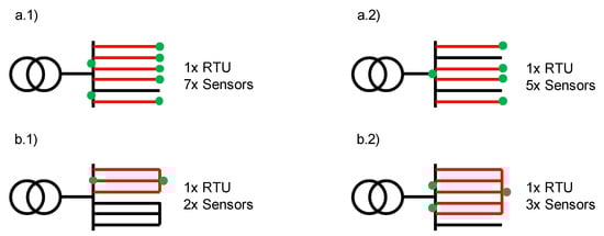
Figure 10.
Examples of consideration of a grid automation system for different topologies with (a.1) radial grid with five overloaded outgoing feeders (OFs), (a.2) radial grid with four overloaded OFs, (b.1) meshed grid with one overloaded mesh and three OFs, and (b.2) meshed grid with one overloaded mesh and five OFs.
Case (a.1) shows a radial grid where five OFs are overloaded, so that the sensors must be considered seven times. Two sensors are needed for the LV side measurement of the five OFs to monitor the loadings and another five sensors at weak points in the respective OFs for voltage measurement. In case (a.2), on the other hand, sensors are only required at a total of five times, since only four OFs are in total overloaded. In case that the DT is overloaded before the necessary sensors are installed from the perspective of the OFs, the sensors are used beforehand. The (n-1)-principle applies to the measurement of the DT, since the last OF can be calculated from all the others. On the other hand, cases (b.1) and (b.2) show two examples of meshed grids. In addition, in each of the four cases one RTU is needed. Actuators are not used at all, since it is assumed that they are available in the CPs and can be used.
5. Planning Measures
If limit violations are identified, they must be eliminated with suitable planning measures. Conventional measures are, therefore, initially implemented as a reference. These are voltage adjustment measures such as the adjustment of the tap at the DT of 2.5% of the voltage twice [32]. In the case of power overloads in particular, cable measures become necessary. This involves the replacement of older cable types, such as NKBA cables, or cross-sections smaller than 150 mm2 in the grid. In the case of more modern cable types with a larger corresponding cross-section, such as NAYY 150 mm2, reinforcement is carried out.
The DLM is used as an innovative measure. If this cannot completely eliminate the limit violations, additional conventional measures are taken.
Since, among other parameters, no information is available on the year of construction of the individual cable sections, this most cost-effective approach was selected. Irrespective of this, it may very well be the case in practice that even cables of a more modern type must be replaced when they reach a certain age.
6. Cost Assumptions and Dataset
In order to reach conclusions about the analyzed grids and to derive recommendations for action, it is important to evaluate the costs of each grid planning variant. For this reason, both the cost assumptions and various calculation variants for implementing the DLM are presented below. After that, the underlying dataset of all LV grids is presented in order to be able to classify the results appropriately.
6.1. Cost Assumptions
Table 6 shows the cost assumptions on which the evaluation is based.
Table 6.
Cost assumptions for low-voltage equipment.
6.2. Different Equipment of the Load Management for Evaluation
For a differentiated evaluation of the DLM as a sensitivity analysis, the following four cost considerations are carried out for the cost calculation of the DLM:
- Full equipment (FE)
- Reduced sensors (RM)
- Basic only (BO); only RTU
- No costs (NC); assumption that information and communication technology is already installed in the grids
FE represents the full equipment when all DLM components need to be set up. RM is used to reduce the number of sensors for voltage measurement at weak points in the OFs. BO assumes that only the RTU is taken into account in terms of costs and NC represents a calculation in which everything for a DLM is already available in the grids, hence, no additional investment costs have to be taken into account.
6.3. Dataset
Table 7 shows the underlying dataset. It shows 13 analyzed LV grids with apportioned charging infrastructure for PrCPs, PuCPs, and HPs for the progressive scenario in 2050. Moreover, the already installed transformer power and the existing building connections and metering points are listed.
Table 7.
Grid structure parameters of the used LV grids for the progressive scenario in 2050.
Note: Although grids G02 and G11 are shown, an analysis of the limit violations showed that neither voltage band violations nor equipment overloads (DT and OFs, respectively) occur in these two grids. Therefore, these two grids are omitted from all further evaluations. It should be noted, however, that these are inner-city LV grids, in which there are no underground garages at apartment buildings.
7. Evaluation and Results
Based on chapter 6, the results from the perspective of the DTs are presented. Then, from the perspective of the OFs, it is shown which line measures are necessary both in the conventional reference variant and in the innovative planning variants with DLM. Finally, the cost assessment with the net present value method is carried out from the combination of both perspectives and the savings potential compared to the reference variant is presented.
7.1. Planning Perspective: Distribution Transformer
Figure 11 shows an evaluation of the equipment overloads of DTs and the required reinforcement. Furthermore, only those DTs are shown which are overloaded in the future. As an example, grid G06 is not shown in this analysis since a total power of 1,200 kVA is installed and no DT overloads occur in any scenario. It can be seen that in addition to the current standard size of 630 kVA, the capacities 800 kVA and 1,000 kVA will also become increasingly necessary for DTs.
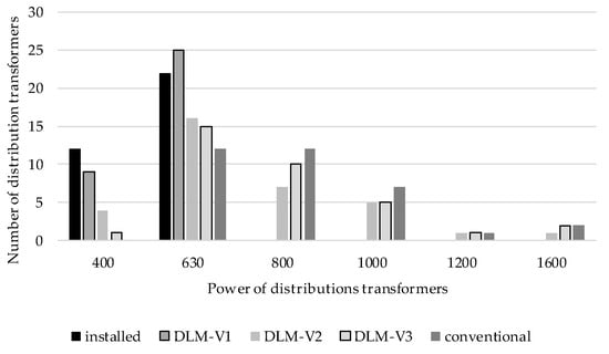
Figure 11.
Power ranges from distribution transformers with and without DLM in case of thermal overloads in the benchmark year 2050 (two scenarios and three HP-Variants).
7.2. Planning Perspective: Outgoing Feeders/Grid Cables
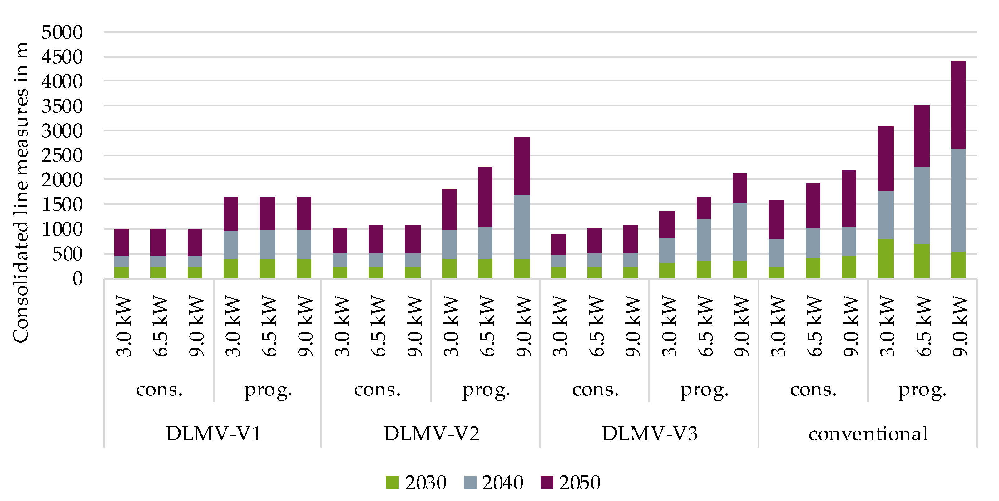
In addition to the necessary increase in transformer power capacity, Figure 12 shows the consolidated line measures required across 11 grids (excluding G02 and G11) in the respective planning variants. It can be seen that the conventional reference variant requires by far the most line measures, whereas a considerable number of lines can be saved with a DLM. However, a more detailed conclusion or recommendation for action can only be derived once a cost evaluation is carried out.
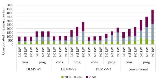
Figure 12.
Necessary line measures for conventional planning and under consideration of a DLM over all cases (two scenarios, three HP-Variants, and three benchmark years).
7.3. Cost Evaluation and Savings Potential
The cost evaluation is performed using the present value method. Briefly explained, it is simply the sum of the present values of capital and operational expenditures per annum (CapEx and OpEx). The present residual values of the grid operating equipment are subtracted from this value, resulting in the present value of all equipment, which is used as the basis for comparison.
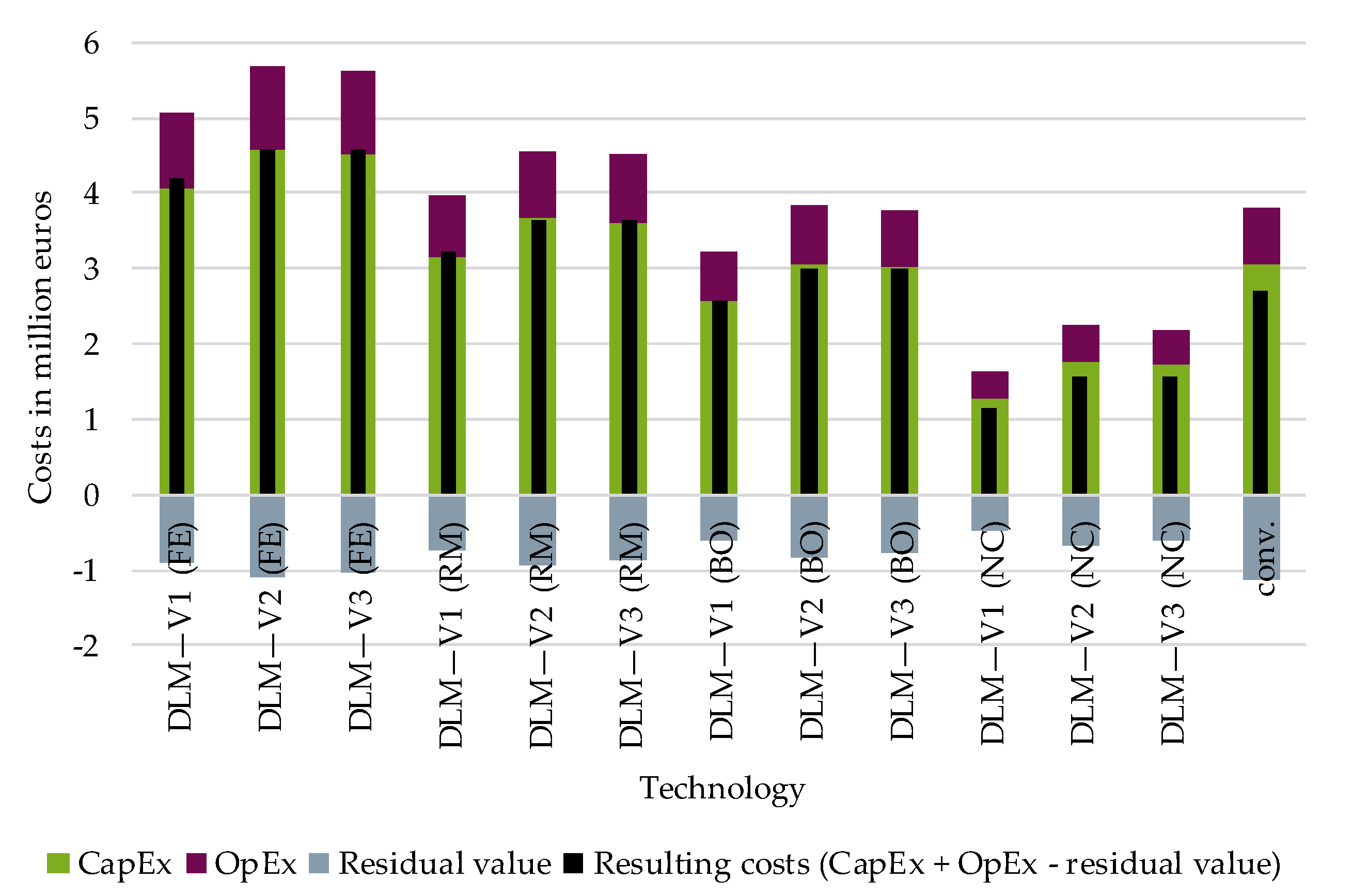
In contrast to the fact described in Section 7.2 that innovative measures within the framework of the DLM can save considerable line measures, Figure 13 shows a different picture when the cost evaluation is included. It shows that almost all DLM variants are more expensive if the DLM requires costs in full or in part. Only when information and communications technology is already available in the grid, this measure becomes more cost-effective than conventional grid expansions.

Figure 13.
Aggregated present values (two scenarios and three heat pump variants) for conventional planning measures as well as DLM-Variants with different cost calculations.
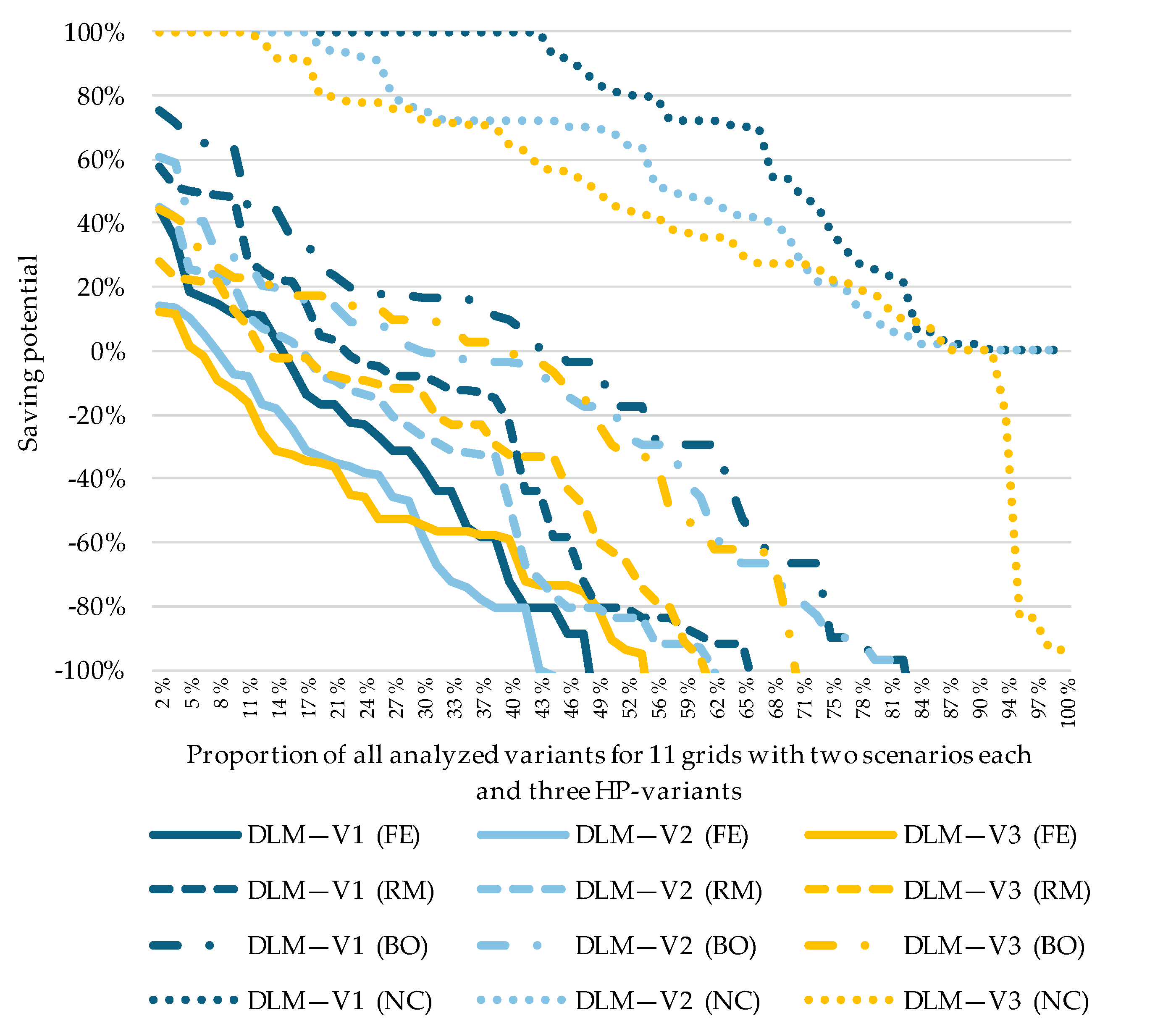
Figure 14 additionally shows the relative savings potential compared to the respective conventional reference variant in all cases separately analyzed (e.g.,: grid G01 6.5 kW conservative, G13 3.0 kW progressive).
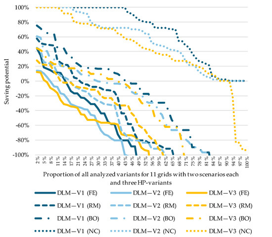
Figure 14.
Savings potential of the DLM-Variants for various cost calculations compared to conventional planning.
Based on the example of DLM-Variant 1 (RM), it becomes clear that in approximately 10% of all analyzed variants, the savings potential is a maximum of 50%, whereas from approximately 22% of all analyzed variants, it becomes more expensive than exclusive conventional planning measures.
Depending on these DLM-Variants, which consider different costs for the DLM, a savings potential of max. 45% is possible. If all the equipment required for a DLM are already installed in the grids, the savings potential increases significantly.
8. Discussion
Based on the methods, framework conditions, and assumptions described above, it can be concluded that load management can reduce the requirement for conventional grid expansions to a considerable extent. Depending on the scenario and variant, it can even completely replace grid expansions, but not in all cases. With the background of the cost assessment carried out, however, it must be stated that load management is currently still too expensive and that conventional grid expansions are, therefore, often preferable. Especially since conventional grid expansions impose little to no loss of convenience for end consumers. However, if the equipment required for a DLM is already available, the savings potential rises significantly and exceeds 70% in approximately 38% of the analyzed cases.
The results of these and other studies can be used as a basis for political discourse on how the load increase due to charging infrastructure for electric mobility and the increasing electrification of the heating sector can be addressed by means of intelligent load management systems in the future and how the costs required for this can be allocated among all stakeholders.
The variants of load management applied in this article can be extended in the future to include other variants, such as the combined curtailment of private and public infrastructure. Furthermore, it can be analyzed what effects a selective and temporary complete shutdown of various CPs has on the planning measures still required in the grid.
Author Contributions
Conceptualization, P.W., S.A.A., K.K., J.M. and B.G.; methodology, P.W., S.A.A. and K.K.; validation, M.Z. and A.S.; formal analysis, J.W.; resources, M.Z.; data curation, P.W. and S.A.A.; writing—original draft preparation, P.W.; writing—review and editing, J.W. and J.M.; supervision, M.Z.; project administration, M.Z.; funding acquisition, M.Z. All authors have read and agreed to the published version of the manuscript.
Funding
This research is a results of the project “PuBStadt” which was funded by the German Federal Ministry for Economic Affairs and Energy following the decision of the “German Bundestag”, grant number 0350038A”.

Acknowledgments
The used data was provided by the six German DSOs Stromnetz Berlin GmbH, Enercity Netzgesellschaft mbH, Rheinische Netzgesellschaft mbH, SachsenNetze GmbH, Stuttgart Netze GmbH and Erlangener Stadtwerke AG.
Conflicts of Interest
The authors declare no conflict of interest. The funders had no role in the design of the study; in the collection, analyses, or interpretation of data; in the writing of the manuscript, or in the decision to publish the results.
References
- Müller, M.; Schulze, Y. Future grid load with bidirectional electric vehicles at home. In Proceedings of the International ETG Congress, Wuppertal, Germany, 18–19 May 2021. [Google Scholar]
- Möller, C.; Kotthaus, C.; Zdrallek, M.; Schweiger, F. Comparison of Incentive Models for Grid-supporting Flexibility Usage of Private Charging Infrastructure. In Proceedings of the International ETG Congress, Wuppertal, Germany, 18–19 May 2021. [Google Scholar]
- Wruk, J.; Cibis, K.; Resch, M.; Sæle, S.; Zdrallek, M. Optimized strategic planning of future norwegian low-voltage networks with a genetic algorithm applying empirical electric vehicle charging data. Electricity 2021, 2, 91–109. [Google Scholar] [CrossRef]
- Ramaswamy, P.C.; Chardonnet, C.; Rapoport, S.; Czajkowski, C.; Sanchez, R.R.; Arriola, I.G.; Bulto, G.O. Impact of electric vehicles on distribution network operation: Real world case studies. In Proceedings of the CIRED Workshop, Helsinki, Finland, 14–15 June 2016. Paper 0415. [Google Scholar]
- Stoeckl, G.; Witzmann, R.; Eckstein, J. Analyzing the Capacity of Low Voltage Grids for Electric Vehicles. In Proceedings of the IEEE Electrical Power and Energy Conference, Winnipeg, MB, Canada, 3–5 October 2011; ISBN 978-1-4577-0404-8. [Google Scholar]
- Propst, A.; Siegel, M.; Braun, M.; Tenbohlen, S. Impacts of electric mobility on distribution grids and possible solution through load management. In Proceedings of the 21st International Conference on Electricity Distribution, Frankfurt, Germany, 6–9 June 2011. Paper 0126. [Google Scholar]
- Schoen, A.; Ulffers, J.; Maschke, H.; Junge, E.; Bott, C.; Thurner, L.; Braun, M. Considering Control Approaches for Electric Vehicle Charging in Grid Planning. In Proceedings of the International ETG Congress, Wuppertal, Germany, 18–19 May 2021. [Google Scholar]
- Zimmerman, L. Progress Report 2018—Market Ramp-Up Phase; German National Platform for Electric Mobility NPE: Berlin, Germany, 2018.
- Bundesministerium für Umwelt, Naturschutz und nukleare Sicherheit BMU. Langfristszenarien und Strategien für den Ausbau der erneuerbaren Energien in Deutschland bei Berücksichtigung der Entwicklung in Europa und global; Bundesministerium für Umwelt, Naturschutz und nukleare Sicherheit BMU: Bonn, Germany, 29 March 2012.
- Shell Deutschland Oil GmbH. Shell Passenger Car Scenarios for Germany to 2040; Shell Deutschland Oil GmbH: Hamburg, Germany, 2014. [Google Scholar]
- Öko-Institut e.V. eMobil 2050; Öko-Institut e.V.: Berlin, Geermany, September 2014. [Google Scholar]
- Institut für Mobilitätsforschung ifmo. Die Zukunft der Mobilität; Institut für Mobilitätsforschung ifmo: Munich, Germany, 2015. [Google Scholar]
- PricewaterhouseCoopers PwC. Autofacts; PricewaterhouseCoopers PwC: Frankfurt on the Main, Germany, September 2016. [Google Scholar]
- Center of Automotive Management CAM. Marktentwicklung von Elektrofahrzeugen für das Jahr 2030; Center of Automotive Management CAM: Bergisch Gladbach, Germany, December 2017. [Google Scholar]
- Fraunhofer-Institut für System-und Innovationsforschung ISI. Entwicklung der regionalen Stromnachfrage und Lastprofile; Fraunhofer-Institut für System-und Innovationsforschung ISI: Karlsruhe, Germany, 17 November 2016. [Google Scholar]
- The Boston Consulting Group BCG. The Electric Car Tipping Point; The Boston Consulting Group BCG: Munich, Germany, January 2018. [Google Scholar]
- BloombergNEF. Electric Vehicle Outlook 2018. 2018. Available online: https://europeanlithium.com/electric-vehicle-outlook-2018-bloomberg/ (accessed on 23 June 2021).
- RBC Capital Markets. Electric Vehicle Forecast Through 2050 & Primer. 2018. Available online: http://www.fullertreacymoney.com/system/data/files/PDFs/2018/May/14th/RBC%20Capital%20Markets_RBC%20Electric%20Vehicle%20Forecast%20Through%202050%20%20Primer_11May2018.pdf (accessed on 23 June 2021).
- Deutsche Energie-Agentur dena. dena-Leitstudie Integrierte Energiewende—Ergebnisbericht; Deutsche Energie-Agentur dena: Berlin, Germany, July 2018. [Google Scholar]
- Bundesverband Wärmepumpe BWP. Branchenstudie 2018: Marktanalyse-Szenarien Handlungsempfehlungen; Bundesverband Wärmepumpe BWP e.V.: Berlin, Germany, 4 December 2018. [Google Scholar]
- Fraunhofer-Institut für Windenergie und Energiesystemtechnik IWES. Wärmewende 2030; Fraunhofer-Institut für Windenergie und Energiesystemtechnik IWES: Kassel, Germany, 2017. [Google Scholar]
- The Boston Consulting Group BCG. Klimapfade für Deutschland; The Boston Consulting Group BCG: Munich, Germany, 2018. [Google Scholar]
- Deutsche Energie-Agentur GmbH dena. Gebäudestudie—Szenarien für eine marktwirtschaftliche Klima- und Ressourcenschutzpolitik 2050 im Gebäudesektor; Deutsche Energie-Agentur GmbH dena: Berlin, Germany, October 2017. [Google Scholar]
- Wirbals, L. Entwicklung und Anwendung von Verteilungsszenarien für Elektrofahrzeuge im städtischen Bereich. Master Thesis, University of Wuppertal, Wuppertal, Germany, 2019. [Google Scholar]
- Wintzek, P. Untersuchung von Rahmenbedingungen und Entwicklung von Szenarien für die Kopplung von städtischen Stromnetzen mit Gas- und Wärmenetzen sowie Entwicklung eines Tools zur Verteilung von Power-to-X-Anlagen. Master Thesis, Trier University of Applied Sciences, Trier, Germany, 2019. [Google Scholar]
- Federal Office of Statistics. Census Database 2011; Federal Office of Statistics: Wiesbaden, Germany, 2011.
- GfK SE Growth from Knowledge. Population structure data; GfK SE Growth from Knowledge: Nuremberg, Germany, 2018. [Google Scholar]
- Plurality and Majority Systems. Available online: www.britannica.com/topic/election-political-science/Plurality-and-majority-systems (accessed on 6 February 2021).
- Monscheidt, J.; Gesmjäger, B.; Slupinski, A.; Yan, X.; Ali, S.A.; Wintzek, P.; Zdrallek, M. An energy demand model for electric load forecast in urban distribution networks. In Proceedings of the CIRED Workshop, Berlin, Germany, 22–23 June 2020. [Google Scholar]
- Wintzek, P.; Ali, S.A.; Talmond, F.; Zdrallek, M.; Röstel, T.; Monscheidt, J.; Gemsjäger, B.; Slupinski, A. Influence of a dynamic load management on the future grid planning of urban low-voltage grids. In Proceedings of the International ETG Congress, Wuppertal, Germany, 18–19 May 2021. [Google Scholar]
- DIN EN 50160:2011-02. Voltage Characteristics of Electricity Supplied by Public Electricity Networks, German version EN 50160:2010 + Corr.:2010 + A1:2015 + A2:2019 + A3:2019; DKE Deutsche Kommission Elektrotechnik Elektronik Informationstechnik in DIN und VDE: Berlin, Germany, 2020. [Google Scholar]
- DIN und VDE. DIN EN 50588-1:2019-12. Medium Power Transformers 50 Hz with Highest Voltage for Equipment Not Exceeding 36 kV—Part 1: General Requirements, German version EN 50588-1:2017; DKE Deutsche Kommission Elektrotechnik Elektronik Informationstechnik in DIN und VDE: Berlin, Germany, 2019. [Google Scholar]


Publisher’s Note: MDPI stays neutral with regard to jurisdictional claims in published maps and institutional affiliations. |
© 2021 by the authors. Licensee MDPI, Basel, Switzerland. This article is an open access article distributed under the terms and conditions of the Creative Commons Attribution (CC BY) license (https://creativecommons.org/licenses/by/4.0/).