
An Efficient Model-Based Clustering via Joint Multiple Sink Placement for WSNs


Abstract
1. Introduction
- We propose a complete model that aims at increasing the network’s lifetime. It performs essential tasks like CH selection (higher Cp factor), path construction from sink to CH (less costly path), and sink placement (in the barycenter of the cluster); as a result, it minimizes the load on the sensor nodes.
- Under the operation of our model, no intermediate node participates or transmits their data packets with less than an energy threshold and more than a distance threshold (long link—discussed in Section 3.1), thereby conserving a significant amount of energy.
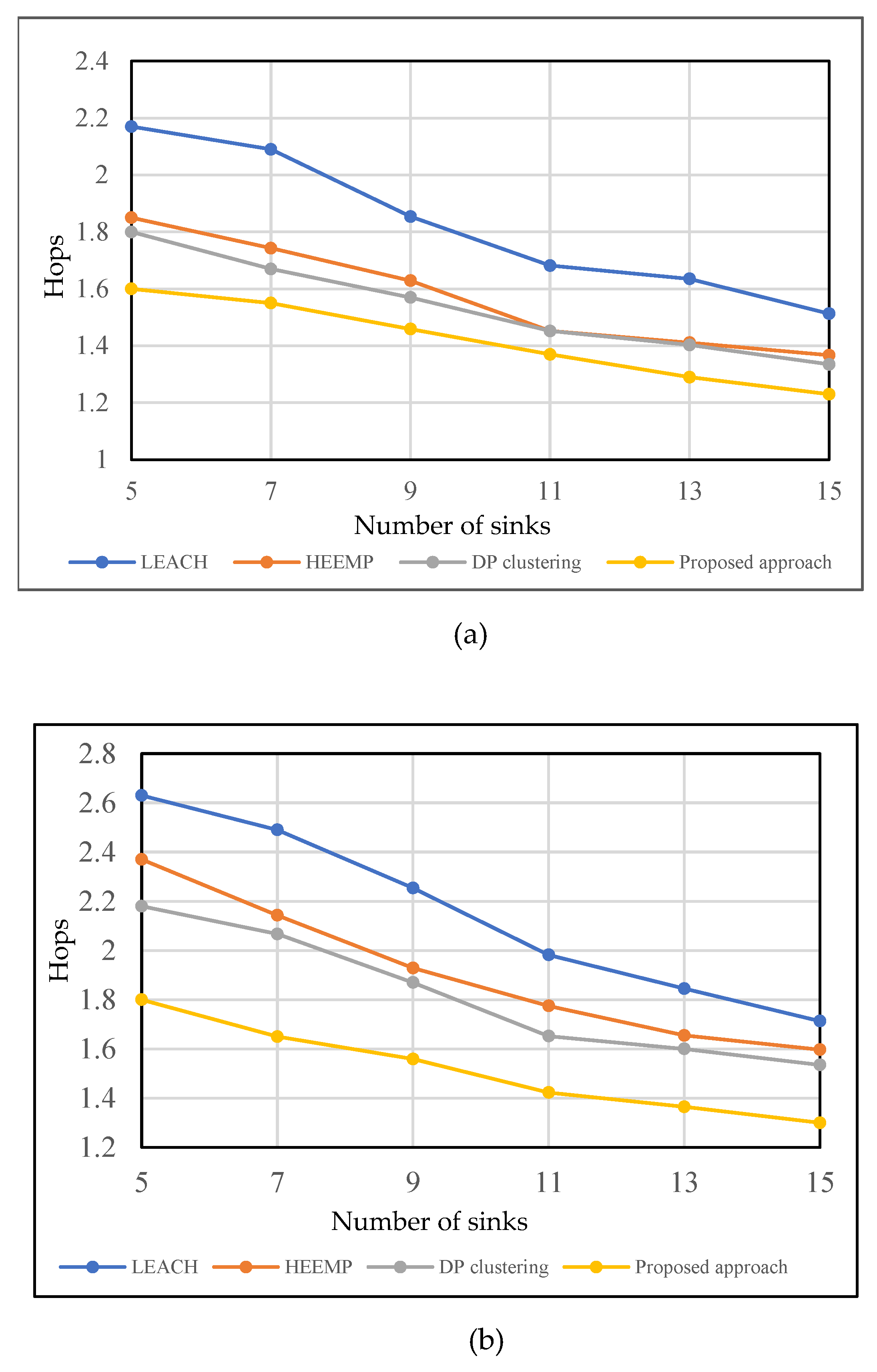
- We compared our proposed technique with others under various simulation settings (varying the number of sensor nodes, CHs, and sinks) to identify areas of limitation and found that it outperformed all of them. We observed that the number of hops is reduced by more than 4% to one hop, and the residual energy is increased by more than 3%.
2. Related Works
2.1. Sink Placement
2.2. Data Transmission and Routing Paths
3. Preliminaries
3.1. Problem Definition
3.2. Ant Clustering Algorithm
3.3. Energy Model
4. Our Proposal
4.1. Deployment Sensors
- Sensor nodes are stationary and are deployed randomly in the environment.
- Multiple sinks (base stations) should be in fixed positions.
- The sensor nodes in the base station’s communication range transmit data directly to the sink.
- The sensor nodes are aware of their neighbours’ node locations.
- The sensor nodes can send and receive data from nodes in the communication range.
- Each sensor node’s total energy consumption cannot exceed its initial energy.
- All sensor nodes have different energies, communications, and sensing ranges.
4.2. Improving the Ant Clustering Algorithm for Sensor Node Clustering
4.2.1. Initialization Step
| Algorithm 1: Initialization phase (IAC) |
|

4.2.2. Main Clustering
| Algorithm 2: main clustering (IAC) | |
| 1. | /*Main loop*/ |
| 2. | for t = 1 to do |
| 3. | for all ants do |
| 4. | If (ant unladen) then |
| 5. | Compute using Equation (13) |
| 6. | Select a random real number [0,1] |
| 7. | If ( then |
| 8. | Pick up |
| 9. | End if |
| 10. | Else |
| 11. | If (ant carrying object) ) then |
| 12. | Find MSCH |
| 13. | Compute using Equation (14) |
| 14. | If ( then |
| 15. | Try to drop near MSCH |
| 16. | .CN ← MSCH .CN |
| 17. | refreshed_memory(ant) |
| 18. | end if |
| 19. | End if |
| 20. | if UnsuccessfulTries > δ then //δ is a predefined threshold |
| 21. | α ← α + ∆α |
| 22. | end if |
| 23. | end for |
| 24. | end for |
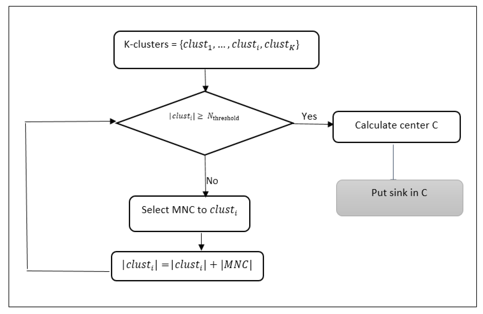
4.3. Sink Placement
- When sink k is located in the barycentre of cluster j:where and are the coordinates of sensor i, which exists in cluster j, is the range communication of sensor i, and is the number of sensors in cluster j.
- When sink k is located in the barycentre of p neighbour clusters:where is the set of p cluster heads of these neighbours’ clusters with communication range , and are the coordinates of cluster head that exists in cluster i, and p is the number of clusters.
4.4. Data Routing and Transmission
| Algorithm 3: Cluster Head Adjustment | |
| Input: | Old_CH |
| Output: | New_CH |
| 1. for each SN in a cluster do | |
| 2. calculate Cp | |
| 3. select node with max Cp | |
| 4. if () ≺ d() | |
| 5. select the following nodes with max Cp | |
| 6. Else | |
| 7. Select as New_CH | |
| 8. End for | |
| Algorithm 4: Repacking _CH_ Route | |
| Declare Drect_nodes_sink = {} | |
| Direct_nodes_CH = {} | |
| Multi_path_R = {} | |
| Multi_path_LR = {} | |
| Multi_path_BR = {} //represents the set of best routes to CH | |
| 1. | for each in nodes |
| 2. | if d() < d() & ( > d( then |
| 3. | Add to Direct_nodes_sink |
| 4. | Else |
| 5. | for each CH do |
| 6. | if ( < ) then |
| 7. | select new CH using Algorithm 3 |
| 8. | If & ( > d( then |
| 9. | Add to Direct_nodes_CH |
| 10. | Else |
| 11. | for each route Rj ∈ Multi_path_R do |
| 12. | if ∀ ∈ Rj: d( ) < then |
| 13. | Multi_path_LR = Multi_path_LR ∪ Rj |
| 14. | End if |
| 15. | End for |
| 16. | for each route LRj ∈ Multi_path_LR |
| 17. | Calculate cost(LRj) using Equation (18) |
| 18. | end for |
| 19. | BR = min(cost(LR)) |
| 20. | Multi_path_BR = Multi_path_BR ∪ BR |
| 21. | End if |
| 22. | End if |
| 23. | End for |
| 24. | End if |
| 25. | end for |
5. Simulation and Evaluation
5.1. Simulation Setup
5.2. Simulation Results
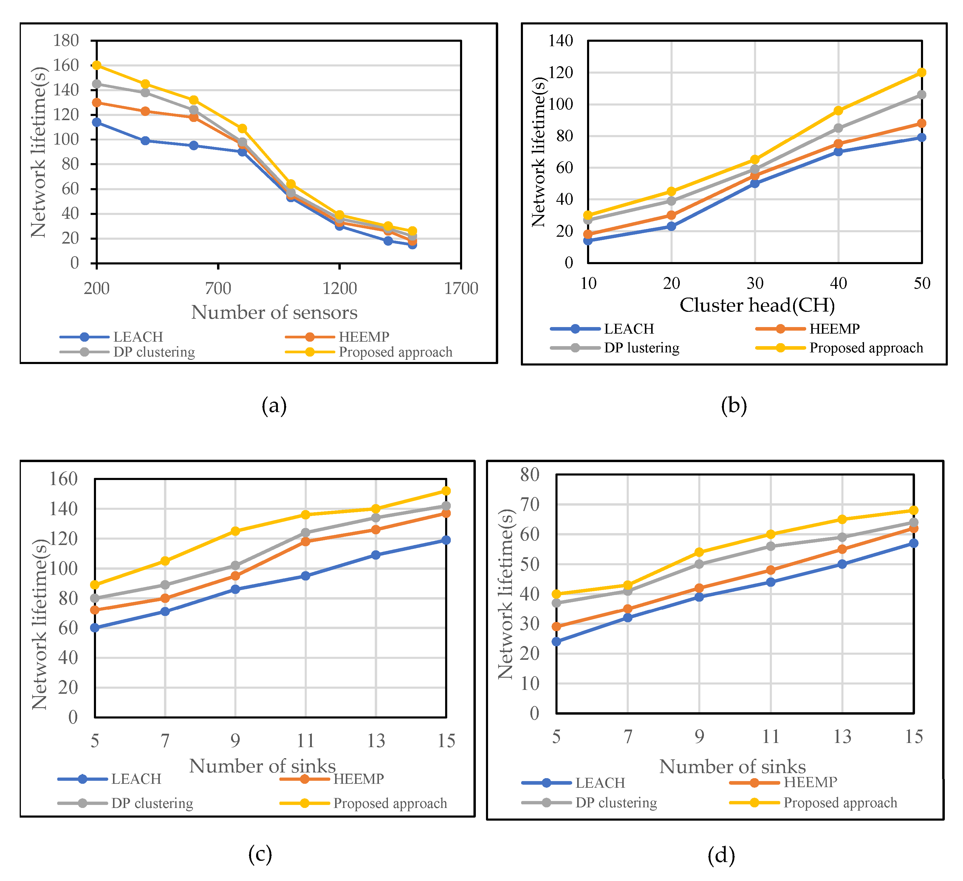
5.2.1. Statistical Results over The Lifetime Based on Various Methods
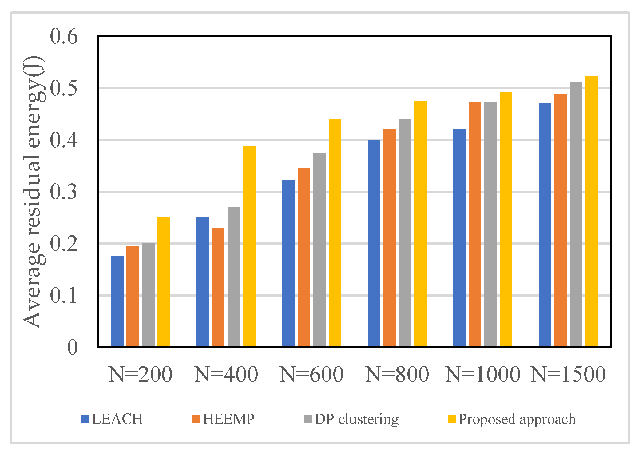
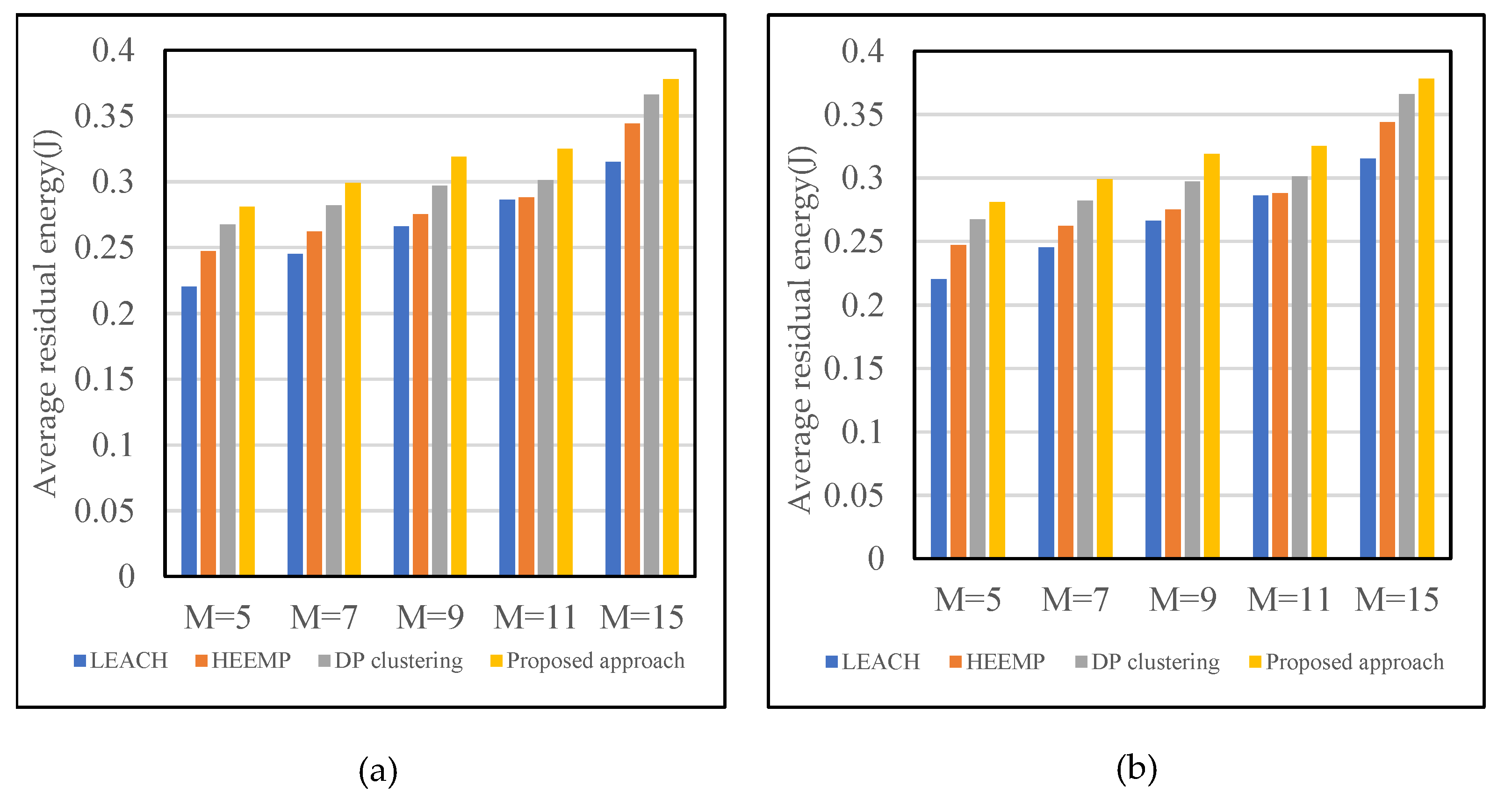
5.2.2. Statistical Results on Average Residual Energy Based on Various Methods
5.2.3. Statistical Results for Hops Based on Various Methods
6. Conclusions
Author Contributions
Funding
Data Availability Statement
Conflicts of Interest
References
- Yousif, M.; Hewage, C.; Nawaf, L. IoT Technologies during and Beyond COVID-19: A Comprehensive Review. Future Internet 2021, 13, 105. [Google Scholar] [CrossRef]
- Wang, Y.; Zen, H.; Sabri, M.F.M.; Wang, X.; Kho, L.C. Towards Strengthening the Resilience of IoV Networks—A Trust Management Perspective. Future Internet 2022, 14, 202. [Google Scholar] [CrossRef]
- Qian, C.; Liu, X.; Ripley, C.; Qian, M.; Liang, F.; Yu, W. Digital Twin—Cyber Replica of Physical Things: Architecture, Applications and Future Research Directions. Future Internet 2022, 14, 64. [Google Scholar] [CrossRef]
- Hackl, J.; Dubernet, T. Epidemic Spreading in Urban Areas Using Agent-Based Transportation Models. Future Internet 2019, 11, 92. [Google Scholar] [CrossRef]
- Autili, M.; Di Salle, A.; Gallo, F.; Pompilio, C.; Tivoli, M. A Choreography-Based and Collaborative Road Mobility System for L’Aquila City. Future Internet 2019, 11, 132. [Google Scholar] [CrossRef]
- Ramakrishnan, A.M.; Ramakrishnan, A.N.; Lagan, S.; Torous, J. From symptom tracking to contact tracing: A framework to explore and assess COVID-19 apps. Future Internet 2020, 12, 153. [Google Scholar] [CrossRef]
- Hyla, T.; Pejaś, J. eHealth Integrity Model Based on Permissioned Blockchain †. Future Internet 2019, 11, 76. [Google Scholar] [CrossRef]
- Hammood, D.A.; Rahim, H.A.; Alkhayyat, A.; Ahmad, R.B. Body-to-Body Cooperation in Internet of Medical Things: Toward Energy Efficiency Improvement. Future Internet 2019, 11, 239. [Google Scholar] [CrossRef]
- Zannou, A.; Boulaalam, A.; Nfaoui, E.H. System service provider–customer for IoT (SSPC-IoT). In Embedded Systems and Artificial Intelligence; Springer: Berlin/Heidelberg, Germany, 2020; pp. 731–739. [Google Scholar]
- Trakadas, P.; Simoens, P.; Gkonis, P.; Sarakis, L.; Angelopoulos, A.; Ramallo-González, A.P.; Skarmeta, A.; Trochoutsos, C.; Calvο, D.; Pariente, T.; et al. An artificial intelligence-based collaboration approach in industrial iot manufacturing: Key concepts, architectural extensions and potential applications. Sensors 2020, 20, 5480. [Google Scholar] [CrossRef]
- Sayeed, A.; Verma, C.; Kumar, N.; Koul, N.; Illés, Z. Approaches and Challenges in Internet of Robotic Things. Future Internet 2022, 14, 265. [Google Scholar] [CrossRef]
- Parada, R.; Palazón, A.; Monzo, C.; Melià-Seguí, J. RFID Based Embedded System for Sustainable Food Management in an IoT Network Paradigm. Future Internet 2019, 11, 189. [Google Scholar] [CrossRef]
- Djukanovic, G.; Kanellopoulos, D.N.; Popovic, G. Evaluation of a UAV-Aided WSN for Military Operations: Considering Two Use Cases of UAV. Int. J. Interdiscip. Telecommun. Netw. (IJITN) 2022, 14, 1–16. [Google Scholar] [CrossRef]
- Sam, A.J.; Mahamuni, C.V. A Wireless Sensor Network (WSN) Prototype for Scouting and Surveillance in Military and Defense Operations using Extended Kalman Filter (EKF) and FastSLAM. SSRN Electron. J. 2022. [Google Scholar] [CrossRef]
- Ahmad, R.; Wazirali, R.; Abu-Ain, T. Machine Learning for Wireless Sensor Networks Security: An Overview of Challenges and Issues. Sensors 2022, 22, 4730. [Google Scholar] [CrossRef] [PubMed]
- Cureau, R.J.; Pigliautile, I.; Pisello, A.L. A New Wearable System for Sensing Outdoor Environmental Conditions for Monitoring Hyper-Microclimate. Sensors 2022, 22, 502. [Google Scholar] [CrossRef] [PubMed]
- Fascista, A. Toward Integrated Large-Scale Environmental Monitoring Using WSN/UAV/Crowdsensing: A Review of Applications, Signal Processing, and Future Perspectives. Sensors 2022, 22, 1824. [Google Scholar] [CrossRef] [PubMed]
- Bouarourou, S.; Boulaalam, A.; Nfaoui, E.H. A bio-inspired adaptive model for search and selection in the Internet of Things environment. PeerJ Comput. Sci. 2021, 7, e762. [Google Scholar] [CrossRef]
- Bouarourou, S.; Zannou, A.; Boulaalam, A.; Nfaoui, E.H. Sensors Deployment in IoT Environment. In Proceedings of the International Conference on Digital Technologies and Applications, Fez, Morocco, 15–20 December 2022; pp. 276–283. [Google Scholar]
- Nazib, R.; Moh, S. Sink-Type-Dependent Data-Gathering Frameworks in Wireless Sensor Networks: A Comparative Study. Sensors 2021, 21, 2829. [Google Scholar] [CrossRef]
- Zannou, A.; Boulaalam, A.; Nfaoui, E.H. SIoT: A New Strategy to Improve the Network Lifetime with an Efficient Search Process. Future Internet 2020, 13, 4. [Google Scholar] [CrossRef]
- Mishra, S.; Thakkar, H. Features of WSN and Data Aggregation techniques in WSN: A Survey. Int. J. Eng. Innov. Technol.(IJEIT) 2012, 1, 264–273. [Google Scholar]
- Oyman, E.; Ersoy, C. Multiple sink network design problem in large scale wireless sensor networks. In Proceedings of the 2004 IEEE International Conference on Communications (IEEE Cat. No.04CH37577), Paris, France, 20–24 June 2004; pp. 3663–3667. [Google Scholar] [CrossRef]
- Safa, H.; Moussa, M.; Artail, H. An energy efficient Genetic Algorithm based approach for sensor-to-sink binding in multi-sink wireless sensor networks. Wirel. Netw. 2013, 20, 177–196. [Google Scholar] [CrossRef]
- Wan, R.; Xiong, N.; Loc, N.T. An energy-efficient sleep scheduling mechanism with similarity measure for wireless sensor networks. Hum. -Cent. Comput. Inf. Sci. 2018, 8, 18. [Google Scholar] [CrossRef]
- Razzaque, M.A.; Dobson, S. Energy-Efficient Sensing in Wireless Sensor Networks Using Compressed Sensing. Sensors 2014, 14, 2822–2859. [Google Scholar] [CrossRef] [PubMed]
- Bangash, J.I.; Abdullah, A.H.; Anisi, M.H.; Khan, A.W. A Survey of Routing Protocols in Wireless Body Sensor Networks. Sensors 2014, 14, 1322–1357. [Google Scholar] [CrossRef] [PubMed]
- Malik, A.; Khan, M.Z.; Faisal, M.; Khan, F.; Seo, J.-T. An Efficient Dynamic Solution for the Detection and Prevention of Black Hole Attack in VANETs. Sensors 2022, 22, 1897. [Google Scholar] [CrossRef] [PubMed]
- Lansky, J.; Ali, S.; Rahmani, A.M.; Yousefpoor, M.S.; Yousefpoor, E.; Khan, F.; Hosseinzadeh, M. Reinforcement Learning-Based Routing Protocols in Flying Ad Hoc Networks (FANET): A Review. Mathematics 2022, 10, 3017. [Google Scholar] [CrossRef]
- Curry, R.M.; Smith, J.C. A survey of optimization algorithms for wireless sensor network lifetime maximization. Comput. Ind. Eng. 2016, 101, 145–166. [Google Scholar] [CrossRef]
- Gawade, R.D.; Nalbalwar, S.L. A Centralized Energy Efficient Distance Based Routing Protocol for Wireless Sensor Networks. J. Sens. 2016, 2016, 1–8. [Google Scholar] [CrossRef]
- Tsoumanis, G.; Oikonomou, K.; Koufoudakis, G.; Aïssa, S. Energy-efficient sink placement in wireless sensor networks. Comput. Netw. 2018, 141, 166–178. [Google Scholar] [CrossRef]
- Jari, A.; Avokh, A. PSO-based sink placement and load-balanced anycast routing in multi-sink WSNs considering compressive sensing theory. Eng. Appl. Artif. Intell. 2021, 100, 104164. [Google Scholar] [CrossRef]
- Heinzelman, W.R.; Chandrakasan, A.; Balakrishnan, H. Energy-efficient communication protocol for wireless microsensor networks. In Proceedings of the 33rd Annual Hawaii International Conference on System Sciences, Maui, Hawaii, 7 January 2000; Volume 2, p. 10. [Google Scholar]
- Ghafoor, S.; Rehmani, M.H.; Cho, S.; Park, S.-H. An efficient trajectory design for mobile sink in a wireless sensor network. Comput. Electron. Eng. 2014, 40, 2089–2100. [Google Scholar] [CrossRef]
- Lindsey, S.; Raghavendra, C. PEGASIS: Power-efficient gathering in sensor information systems. In Proceedings of the Aerospace Conference Proceedings, Big Sky, MT, USA, 9–16 March 2002; Volume 3, pp. 1125–1130. [Google Scholar]
- Han, Z.; Wu, J.; Zhang, J.; Liu, L.; Tian, K. A general self-organized tree-based energy-balance routing protocol for wireless sensor network. IEEE Trans. Nucl. Sci. 2014, 61, 732–740. [Google Scholar] [CrossRef]
- Pantazis, N.A.; Nikolidakis, S.A.; Vergados, D.D. Energy-Efficient Routing Protocols in Wireless Sensor Networks: A Survey. IEEE Commun. Surv. Tutor. 2012, 15, 551–591. [Google Scholar] [CrossRef]
- Sajwan, M.; Gosain, D.; Sharma, A.K. Hybrid energy-efficient multi-path routing for wireless sensor networks. Comput. Electron. Eng. 2018, 67, 96–113. [Google Scholar] [CrossRef]
- Bonabeau, E.; Dorigo, M.; Theraulaz, G.; Theraulaz, G. Swarm Intelligence: From Natural to Artificial Systems; Oxford University Press: Oxford, UK, 1999. [Google Scholar]
- Sarathy, R.; Shetty, B.; Sen, A. A constrained nonlinear 0–1 program for data allocation. Eur. J. Oper. Res. 1997, 102, 626–647. [Google Scholar] [CrossRef]
- Handl, J.; Meyer, B. Ant-based and swarm-based clustering. Swarm Intell. 2007, 1, 95–113. [Google Scholar] [CrossRef]
- Jevtić, A. Swarm intelligence: Novel tools for optimization, feature extraction, and multi-agent system modeling. Telecomunicacion. Ph.D. Thesis, Technical University of Madrid, Madrid, Spain, 2011. [Google Scholar]
- Jevtić, A.; Quintanilla-Domínguez, J.; Barrón-Adame, J.M.; Andina, D. Image segmentation using ant system-based clustering algorithm. In Proceedings of the Soft Computing Models in Industrial and Environmental Applications, 6th International Conference SOCO 2011, Bilbao, Spain, 22–24 September 2011; pp. 35–45. [Google Scholar]
- Dorigo, M.; Birattari, M. Swarm intelligence. Scholarpedia 2007, 2, 1462. [Google Scholar] [CrossRef]
- Cui, X.; Potok, T.E.; Palathingal, P. Document clustering using particle swarm optimization. In Proceedings of the 2005 IEEE Swarm Intelligence Symposium, Pasadena, CA, USA, 8–10 June 2005; SIS 2005. pp. 185–191. [Google Scholar]
- Zhao, C.; Wu, C.; Wang, X.; Ling, B.W.-K.; Teo, K.L.; Lee, J.-M.; Jung, K.-H. Maximizing lifetime of a wireless sensor network via joint optimizing sink placement and sensor-to-sink routing. Appl. Math. Model. 2017, 49, 319–337. [Google Scholar] [CrossRef]
- Kabakulak, B. Sensor and sink placement, scheduling and routing algorithms for connected coverage of wireless sensor networks. Ad Hoc Netw. 2019, 86, 83–102. [Google Scholar] [CrossRef]
- Hong, Z.; Wang, R.; Li, X. A clustering-tree topology control based on the energy forecast for heterogeneous wireless sensor networks. IEEE/CAA J. Autom. Sin. 2016, 3, 68–77. [Google Scholar] [CrossRef]
- Mukherjee, S.; Amin, R.; Biswas, G.P. Design of routing protocol for multi-sink based wireless sensor networks. Wirel. Netw. 2019, 25, 4331–4347. [Google Scholar] [CrossRef]
- Cayirpunar, O.; Tavli, B.; Kadioglu-Urtis, E.; Uludag, S. Optimal Mobility Patterns of Multiple Base Stations for Wireless Sensor Network Lifetime Maximization. IEEE Sens. J. 2017, 17, 7177–7188. [Google Scholar] [CrossRef]
- Sapre, S.; Mini, S. A differential moth flame optimization algorithm for mobile sink trajectory. Peer—Peer Netw. Appl. 2020, 14, 44–57. [Google Scholar] [CrossRef]
- Gosain, D.; Snigdh, I.; Sajwan, M. DSERR: Delay Sensitive Energy Efficient Reliable Routing Algorithm. Wirel. Pers. Commun. 2017, 97, 3685–3704. [Google Scholar] [CrossRef]
- Sohraby, K.; Minoli, D.; Znati, T. Wireless sensor networks: Technology Protocols; Applications; John Wiley & Sons: Hoboken, NJ, USA, 2007. [Google Scholar]
- Heinzelman, W.R.; Kulik, J.; Balakrishnan, H. Adaptive protocols for information dissemination in wireless sensor networks. In Proceedings of the 5th annual ACM/IEEE International Conference on Mobile Computing and Networking, Washington, DC, USA, 15–20 August 1999; pp. 174–185. [Google Scholar]
- Akyildiz, I.F.; Su, W.; Sankarasubramaniam, Y.; Cayirci, E. Wireless sensor networks: A survey. Comput. Netw. 2002, 38, 393–422. [Google Scholar] [CrossRef]
- Handy, M.; Haase, M.; Timmermann, D. Low energy adaptive clustering hierarchy with deterministic cluster-head selection. In Proceedings of the 4th International Workshop on Mobile and Wireless Communications Network, Lake Buena Vista, FL, USA, 21–23 May 2003. [Google Scholar] [CrossRef]
- Manjeshwar, A.; Agrawal, D.P. TEEN: ARouting Protocol for Enhanced Efficiency in Wireless Sensor Networks. ipdps 2001, 1, 189. [Google Scholar]
- Tirani, S.P.; Avokh, A. On the performance of sink placement in WSNs considering energy-balanced compressive sensing-based data aggregation. J. Netw. Comput. Appl. 2018, 107, 38–55. [Google Scholar] [CrossRef]
- Sun, P.; Wu, L.; Wang, Z.; Xiao, M.; Wang, Z. Sparsest Random Sampling for Cluster-Based Compressive Data Gathering in Wireless Sensor Networks. IEEE Access 2018, 6, 36383–36394. [Google Scholar] [CrossRef]
- Zannou, A.; Boulaalam, A.; Nfaoui, E.H. Data Flow Optimization in the Internet of Things. Stat. Optim. Inf. Comput. 2022, 10, 93–106. [Google Scholar] [CrossRef]
- Lumer, E.D.; Faieta, B. Diversity and adaptation in populations of clustering ants. In Proceedings of the Third International Conference on Simulation of Adaptive Behavior: From Animals to Animats 3: From Animals to Animats 3, Brighton, UK, 8–12 August 1994; pp. 501–508. [Google Scholar]
- Deneubourg, J.-L.; Goss, S.; Franks, N.; Sendova-Franks, A.; Detrain, C.; Chrétien, L. The dynamics of collective sorting robot-like ants and ant-like robots. In From Animals to Animats: Proceedings of the First International Conference on Simulation of Adaptive Behavior; MIT Press: Cambridge, MA, USA, 1990; pp. 356–365. [Google Scholar]
- Nanda, S.J.; Panda, G. A survey on nature inspired metaheuristic algorithms for partitional clustering. Swarm EComput. 2014, 16, 1–18. [Google Scholar] [CrossRef]
- Grover, A.; Leskovec, J. node2vec: Scalable feature learning for networks. In Proceedings of the 22nd ACM SIGKDD International Conference on Knowledge Discovery and Data Mining, San Francisco, CA, USA, 13–17 August 2016; pp. 855–864. [Google Scholar]


| Authors \Year | Sink Type | Number of Sinks | Clustering Mechanism | Network Constraints Considered | Keys Points: Algorithms /Protocols | Limitation/ Constraint | ||
|---|---|---|---|---|---|---|---|---|
| Network Lifetime | Energy Consumption | Data Routing | ||||||
| Sapre et al. (2021) [52] | mobile | single | √ | √ | √ | √ | Combines meta-heuristic differential moth flame optimization (MFO) and differential evolution (DE) as DMFO to place the relay nodes to cluster the WSN. | Coverage time has not been considered in this model. As a result, it impacts the lifetime performance of sensor networks. |
| Kabakulak (2019) [48] | static | multiple | × | √ | √ | √ | SPSRC, a mixed integer programming formulation, determines the best placement for sensors and sinks, as well as sensor active/standby times and data transmission paths from each active node to its assigned sink. | This method assigns the task of selecting alive nodes to lower energy sensor nodes; this raises dead nodes and breaks network connections. |
| Tsoumanis et al. (2018) [32] | static | multiple | × | √ | √ | × | A k-median facility location problem. | Focus only on sink deployment. |
| Cayirpunar (2017) [51] | mobile | multiple | × | √ | √ | √ | The mixed integer programming (MIP) framework defines network lifetime (NL) for multiple mobile BSs under various mobility patterns. | The method fails to determine the data transmission delay and throughput. |
| Zhao et al. (2017) [47] | static | multiple | √ | √ | √ | √ | Sink location and sensor-to-sink route optimization using the PSO algorithm. | The protocol is limited to sinks in the monitoring zone. |
| Hong et al. (2016) [49] | static | multiple | √ | √ | √ | × | CTEF is a clustering-tree topology control technique based on the energy forecast for conserving energy and guaranteeing network load balancing while considering connection quality and packet loss rate. | This solution does not address the issue of data transmission delay. |
| Ghafoor et al. (2014) [35] | Mobile | single | × | √ | √ | √ | Based on the Hilbert curve, a mobile sink trajectory is created. | Collecting data in the direction of the Hilbert curve does not guarantee that the load on the network’s nodes will be balanced and energy consumption will rise. |
| Oyman et al. (2004) [23] | static | Multiple | √ | √ | √ | × | Sink placement using the k-means algorithm. | The method is unsuitable for large-scale networks, and the pathway from sensors to sinks must be considered. |
| Authors\ Year | Approach | Clustering Mechanism | Network Constraints Considered | CH Selection Criteria | Data Transmission | Drawbacks/Limitations | |
|---|---|---|---|---|---|---|---|
| Network Lifetime | Energy Consumption | ||||||
| Zannou et al. (2022) [61] | DP clustering | √ | √ | √ | -Coordinate’s location of the node. | Multi-hop | It is likely to select a low-energy node as CH. |
| Sajwan et al. (2018) [39] | HEEMP | √ | √ | √ | -Residual energy -Node degree | Multi-hop | The nodes near the CH node in the proposed multi-hop intra-cluster communications receive multiple messages and collect them without considering whether they can handle the load or not. |
| Jari et al. (2018) [33] | MPAR& EMPAR | √ | √ | √ | -Residual energy -distance | Multi-hop | The network becomes costly when several sinks are involved. Finding the best position becomes increasingly challenging as the number of sinks increases. |
| Pantazis et al. (2018) [38] | CDG | √ | √ | √ | -At the centre of evenly divided regions | Multi-hop | It considers network properties, but ignores CDG features. |
| Gawade et al. (2016) [31] | CEED | √ | √ | √ | -Dissipation energy of node -Distance to sink | Multi-hop | It puts a tremendous load on CH. |
| Han et al. (2014) [37] | GSTEB | √ | √ | √ | -Maximum residual energy (as root node) | Multi-hop | It consumes more energy due to direct routing. The significant number of control packets has a higher energy overhead. |
| Lindsey et al. (2012) [36] | PEGASIS | √ | √ | √ | -Each node selected as a leader | Multi-hop | There is a significant delay for remote nodes, and the single leader mechanism can generate congested. |
| Heinzelman et al. (2000) [34] | DT | √ | √ | √ | -Random threshold | Multi-hop | It ignores the distance between the Cluster Head and the BS. |
| Notation | Description |
|---|---|
| Number of sensor nodes | |
| M | Number of sinks |
| The sensor i | |
| ) | Distance between the sensor and the sensor . |
| min_d() | Minimum Distance between the sensor and the sensor . |
| All cluster head nodes in the network. | |
| BS | Base station/Sink. |
| Cluster head of the cluster. | |
| Chance of picking a node i factor. | |
| () | Communication range between a node and the node. |
| The cluster. | |
| | | Number of nodes in the cluster i. |
| S(i) | A set of alive neighboors of node i. |
| MNC | The most neighbors clusters. |
| Number of nodes in the cluster MNC. | |
| Rj | The multi path route. |
| BR | The route between CH and a node with minimum cost value (Best Route). |
| The residual energy. | |
| The minimum residual energy in the considering network. | |
| The maximum residual energy in the considering network. | |
| The energy required for reception data. | |
| The energy required for transmission data. | |
| The energy required in multi path model. | |
| The energy required in Direct path model. | |
| Number of ants | |
| Number of iterations |
| Parameters | Values |
|---|---|
| N | 1000 |
| M | 13 |
| CH | 30 |
| 500 | |
| 0.5 | |
| S | 30 m × 30 m |
| 0.05 | |
| 0.1 | |
| 0.15 | |
| 500 | |
| 0.3 J | |
| 0.9 J | |
| 20 nJ/bit | |
| 45 nJ/bit | |
| [10 m, 30 m] | |
| 30 m | |
| 0.2J |
| Approach | Number of Nodes with 1-Hop (%) | Number of Nodes with 2-Hop (%) | Number of Nodes with 3-Hop (%) | Number of Nodes with 4-Hop (%) | Number of Nodes with 5-Hop (%) |
|---|---|---|---|---|---|
| LEACH [57] | 87.2 | 4.8 | 3.5 | 2.5 | 2 |
| HEEMP [39] | 92.5 | 3.5 | 2.5 | 1.5 | 0 |
| DP clustering [61] | 93.5 | 3.5 | 2.8 | 0.2 | 0 |
| Our proposed | 96.5 | 2 | 1.5 | 0 | 0 |
Disclaimer/Publisher’s Note: The statements, opinions and data contained in all publications are solely those of the individual author(s) and contributor(s) and not of MDPI and/or the editor(s). MDPI and/or the editor(s) disclaim responsibility for any injury to people or property resulting from any ideas, methods, instructions or products referred to in the content. |
© 2023 by the authors. Licensee MDPI, Basel, Switzerland. This article is an open access article distributed under the terms and conditions of the Creative Commons Attribution (CC BY) license (https://creativecommons.org/licenses/by/4.0/).
Share and Cite
Bouarourou, S.; Zannou, A.; Nfaoui, E.H.; Boulaalam, A. An Efficient Model-Based Clustering via Joint Multiple Sink Placement for WSNs. Future Internet 2023, 15, 75. https://doi.org/10.3390/fi15020075
Bouarourou S, Zannou A, Nfaoui EH, Boulaalam A. An Efficient Model-Based Clustering via Joint Multiple Sink Placement for WSNs. Future Internet. 2023; 15(2):75. https://doi.org/10.3390/fi15020075
Chicago/Turabian StyleBouarourou, Soukaina, Abderrahim Zannou, El Habib Nfaoui, and Abdelhak Boulaalam. 2023. "An Efficient Model-Based Clustering via Joint Multiple Sink Placement for WSNs" Future Internet 15, no. 2: 75. https://doi.org/10.3390/fi15020075
APA StyleBouarourou, S., Zannou, A., Nfaoui, E. H., & Boulaalam, A. (2023). An Efficient Model-Based Clustering via Joint Multiple Sink Placement for WSNs. Future Internet, 15(2), 75. https://doi.org/10.3390/fi15020075