Abstract
Community-managed forests within agroforestry landscapes are vital for both carbon sequestration and agricultural sustainability. This study assesses the Hariyali Community Forest (HCF) in western Nepal, emphasizing its role in carbon storage within a Sal (Shorea robusta)-dominated lowland forest containing diverse native and medicinal species. Stratified field inventories combined with satellite-derived biomass and land-use/land-cover data were used to quantify carbon stocks and spatial trends. In 2022, the mean aboveground carbon density was 165 tC ha−1, totaling approximately 101,640 tC (~373,017 tCO2e), which closely matches satellite-based trends and indicates consistent carbon accumulation. Remote sensing from 2015–2022 showed a net tree cover gain of 427 ha compared to a 2000 baseline of 188 ha, evidencing effective community-led regeneration. The 615 ha Sal-dominated landscape also sustains agroforestry, small-scale horticulture, and subsistence crops, integrating livelihoods with conservation. Temporary carbon declines between 2020 and 2022, linked to localized harvesting and management shifts, highlight the need for stronger governance and local capacity. This study, among the first integrated carbon assessments in Nepal’s lowland Sal forests, demonstrates how community forestry advances REDD+ (Reducing Emissions from Deforestation and Forest Degradation, and the role of conservation, sustainable management of forests, and enhancement of forest carbon stocks in developing countries) objectives while enhancing rural resilience. Linking field inventories with satellite-derived biomass and land-cover data situates community forestry within regional environmental change and SDG (Sustainable Development Goals) targets (13, 15, and 1) through measurable ecosystem restoration and livelihood gains.
1. Introduction
Carbon sequestration, the capture and long-term storage of atmospheric carbon dioxide (CO2), is a critical natural mechanism for mitigating anthropogenic climate change [1,2]. Forest ecosystems are among the most important terrestrial carbon sinks, absorbing CO2 through photosynthesis and storing it in vegetation, litter, and soil. Globally, forests sequester approximately 2.6 ± 0.5 gigatons of carbon annually, accounting for nearly 90% of terrestrial biomass carbon and over 70% of soil organic carbon stocks [3,4].
However, these carbon pools are increasingly at risk due to LULC (Land Use Land Cover) changes, particularly deforestation, agricultural expansion, and urbanization [5]. Human-induced land-cover transitions, such as forest conversion to agriculture, fragmentation, or selective logging, can significantly modulate carbon storage. Depending on their type and intensity, these transitions may either diminish or enhance carbon sinks [6]. Reference [7] mapped global forest carbon fluxes and showed that disturbances and regrowth dynamics critically influence net carbon outcomes [8]. Similarly, studies in tropical ecosystems have shown that specific land-cover transitions can lead to substantial reductions in both biodiversity and carbon stocks, highlighting the ecological significance of forest state changes [9]. Recent assessments from comparable Asian mountain landscapes similarly reveal that land-use shifts such as expanding settlements and forest removal significantly reduce carbon stocks and result in measurable economic losses [10].
To counter these pressures, Nepal launched its Community Forestry Program (CFP) in the late 1970s, institutionalized through the 1982 Decentralization Act and the 1993 Forest Act [11]. Under this model, national forests are handed over to Community Forest User Groups (CFUGs), empowering local communities to manage and conserve forests for collective benefit. These forests provide not only environmental services, such as carbon sequestration and biodiversity protection, but also direct livelihood benefits including fuelwood, timber, fodder, and non-timber forest products (NTFPs) like wild fruits, medicinal herbs, and fibers [12]. By 2012, over 18,000 CFUGs were managing 2.4 million hectares of forest, involving 2.9 million households [13]. In addition to timber and non-timber products, community forests in Nepal contribute to local food systems through integrated agroforestry practices, seasonal horticulture, and the cultivation of subsistence crops in buffer zones, creating synergies between agricultural productivity and forest conservation.
As of 2024, the number has grown to 23,682 CFUGs, managing approximately 24,902 km2, which is around 37.7% of Nepal’s total forest area [14]. This community-led conservation model has been pivotal in increasing national forest cover, which rose from about 29% in the late 1990s to over 40% by 2020 [15,16,17,18].
The carbon sequestration potential of Nepal’s community forests is estimated at 2.79 tC ha−1 yr−1 [19], and studies confirm their role in reducing deforestation and improving forest health [20,21,22]. However, spatial variability in carbon outcomes persists due to localized LULC shifts, socio-economic dynamics, and uneven implementation of forest policies. This highlights the need for site-specific analysis of forest change and carbon dynamics to inform adaptive forest governance and support Nepal’s nationally determined contributions (NDCs) under the Paris Agreement.
Community stewardship has significantly improved HCF’s tree density, canopy cover, and species richness. However, the recent implementation of Scientific Forest Management (SFM) led to temporary biomass loss due to poor planning and limited oversight. In this context, community forests like HCF have growing potential to contribute to climate mitigation through REDD+ mechanisms and voluntary carbon markets, while also strengthening rural livelihoods and ecological resilience.
While community forestry in Nepal has been widely examined for its ecological and social outcomes [23,24,25,26], few studies have systematically integrated stratified field-based carbon inventories with satellite-derived biomass and temporal land-use/land-cover (LULC) trends, particularly in lowland Sal (Shorea robusta) forests. Studies have clearly demonstrated the comparative utility of different satellite-derived land cover datasets for forest monitoring, highlighting the respective advantages and limitations of products such as Phased Array type L-band Synthetic Aperture Radar-Forest/Non-Forest (PALSAR-FNF), Environmental Systems Research Institute (ESRI) Land Cover, and Google’s Dynamic World. These tools have shown promise in regional forest assessments and may enhance the accuracy of carbon accounting when integrated with ground validation. Similarly, spatiotemporal studies on forest carbon dynamics in managed forest units underscore the importance of integrating high-resolution temporal data with local forest management records [27,28].
This study addresses that gap by combining high-resolution field data with multi-temporal remote sensing to assess spatiotemporal variability in aboveground carbon under community management. Building on recent evidence highlighting the contribution of community-led conservation to climate resilience [29,30,31,32], it offers a site-specific, empirically validated, and replicable approach to forest carbon accounting within a critical transboundary biodiversity corridor. This study aims to provide an integrated assessment of aboveground carbon dynamics and community stewardship in a lowland Sal-dominated forest of western Nepal. The specific objectives were to:
- (1)
- Quantify aboveground carbon stocks across vegetation strata of the Hariyali Community Forest using stratified field inventories and species-specific allometric models.
- (2)
- Examine multi-temporal trends in forest biomass and carbon dynamics (2010–2022) through the integration of satellite-derived biomass datasets with ground-based measurements.
- (3)
- Analyze land-use and land-cover (LULC) transitions to evaluate how community management and regeneration have influenced spatial patterns of forest recovery and carbon accumulation.
- (4)
- Derive management and policy implications for adaptive community forestry, emphasizing data-driven carbon monitoring, sustainable harvesting, and alignment with REDD+ and Nepal’s NDC targets.
2. Study Area
Hariyali Community Forest is situated in Kanchanpur District, Far-West Province, Nepal (Figure 1). The district spans 161,741 hectares, with coordinates ranging from 28°50′00″ N to 28°52′30″ N latitude and 80°26′00″ E to 80°28′30″ E longitude. Elevation varies between 160 m and 255 m above sea level. The forest covers 614.88 hectares and is dominated by Sal (Shorea robusta), followed by Ashna (Terminalia tomentosa). According to the National Statistics Office of Nepal [33], the Hariyali Community Forest area comprises 1503 households and a total population of 6493 as of 2021.
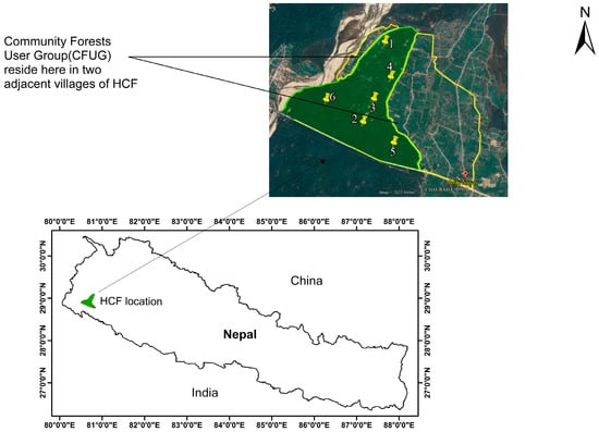
Figure 1.
Location map of the study area with six sample plots.
Located within a protected, forest-rich zone, Hariyali Community Forest plays a critical ecological role as part of a biological corridor in the Kanchanpur District. This corridor connects four Rural Municipalities, Raikwar-Bichawa, Baisi-Bichawa, Shankarpur, and Krishnapur, and links Nepal’s Churia forests in the north with India’s Dudhwa National Park in the south. It also forms part of a transboundary conservation landscape between Dudhwa National Park and Shuklaphanta Wildlife Reserve.
This study focuses on HCF, located in Krishnapur Municipality of Kanchanpur District, within the ecologically vital Laljhadi–Mohona Biological Corridor. This corridor forms a critical wildlife linkage between Nepal’s Churia range and India’s Dudhwa National Park. HCF is dominated by Sal (Shorea robusta), with associated species like Ashna (Terminalia tomentosa), Harro (Terminalia chebula), and Timur (Zanthoxylum armatum). It supports endangered fauna such as the Asian elephant (Elephas maximus) and Royal Bengal tiger (Panthera tigris tigris), providing breeding, migratory, and foraging habitat critical for regional biodiversity. The following six circular sample plots, including dense and sparse strata, were studied.
Within this corridor, the two adjoining villages, Belkundi (on the left in the study area map) and Mawafata (on the right), host the Community Forest User Group (CFUG) that manages Hariyali Community Forest (Figure 1) [https://www.google.com/earth/] accessed on 24 April 2025.
The region experiences a subtropical climate characterized by hot summers, mild winters, and distinct wet and dry seasons. According to climate data from the Dhangadhi (Attariya) station (Department of Hydrology and Meteorology, Nepal), summer temperatures (March–June) range from 30–40 °C, while the monsoon season (June–September) brings slightly cooler temperatures of 25–35 °C. Winter months (November–February) see temperatures drop to 15–25 °C, with occasional nighttime lows of 5–10 °C. Annual precipitation ranges from 1500 to 2000 mm, with the majority falling during the monsoon season. The remaining months, especially October to May, remain relatively dry. High humidity and sporadic flooding during the rainy season are notable features, underscoring the importance of accounting for seasonal variability when managing vegetation and hydrology in the adjacent Laljhadi–Mohona Corridor.
Adjacent farmlands incorporate agroforestry systems, where farmers intercrop fruit trees, fodder species, and annual crops, thereby enhancing both food security and the potential for carbon sequestration in the broader landscape. Resource use within the forest is regulated: extraction of stone, sand, and aggregates is permitted in a controlled manner, either consumed locally or sold beyond the user group, in line with the Initial Environmental Examination (IEE) report approved by Krishnapur Municipality. Meanwhile, households from the adjacent villages are permitted to collect mud, fodder, leaves, and fuelwood within specified time frames, in accordance with CFUG guidelines and under the supervision of the Division Forest Office, thereby balancing subsistence needs with ecological sustainability.
The Laljhadi–Mohona Corridor exemplifies a regional environmental change hotspot, where shifting climatic patterns, forest use, and agricultural practices converge. Understanding the forest–agriculture interface here provides insight into how local management decisions scale up to influence regional carbon balances and ecological connectivity across the Himalayan foothills.
3. Materials and Methods
This study employed an integrated methodological framework combining participatory field inventory, satellite-based carbon estimation, and LULC analysis to assess aboveground carbon (AGC) dynamics in the HCF. The research workflow is summarized in Figure 2.
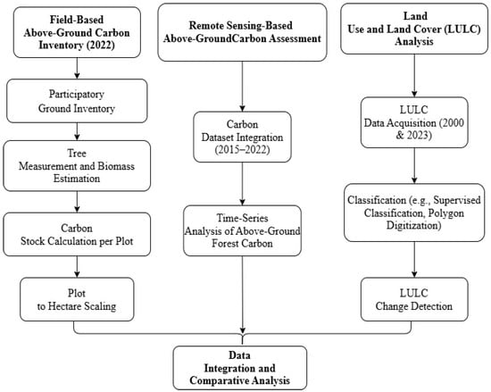
Figure 2.
Research workflow for Estimation of Above-Ground Carbon Stock Changes.
3.1. Field-Based Above-Ground Carbon Inventory (2022)
3.1.1. Participatory Ground Inventory
In April 2022, a participatory field inventory was conducted in HCF, situated north of the Mahendra Highway in Kanchanpur District, Nepal. We conducted the forest inventory jointly with a team of subject experts (as mentioned in the acknowledgement) in collecting tree data, including species, diameter at breast height (DBH), height, and plot location. This participatory approach improved data accuracy and fostered community ownership.
The carbon stock per plot was calculated using tree allometric equations, scaled to a per-hectare basis, and supported by secondary data from the Department of Hydrology and Meteorology, the Central Bureau of Statistics (CBS), and other relevant institutions.
3.1.2. Stratification and Sampling Design
To reduce variability and improve accuracy, the forest was stratified into two relatively homogeneous strata based on canopy density (>70% canopy cover = dense, <70% = sparse), dominant species, slope, altitude, and aspect [34,35]. Using stratified random sampling, six circular plots (0.025 ha each) were established, three per stratum, resulting in a total sampling intensity of 0.05%. Although the sampling intensity was low, stratification minimized bias, and homogeneity in canopy structure suggested that six plots were sufficient for baseline estimates. Nonetheless, we recognize this as a limitation and recommend higher plot density or UAV-based sampling for future research.
Our sampling design followed Nepal’s Community Forest Inventory Guideline (DoF, 2061 BS), which recommends flexible sampling intensities of 0.2%–1.5% depending on forest size, heterogeneity and logistical feasibility. Larger community forests are commonly inventoried using sampling fractions toward the lower end of this range, particularly when preliminary stratification indicates structural homogeneity. This practice is consistent with empirical studies from Nepal, where community-forest biomass inventories have applied 0.5%–1% sampling intensity or modest numbers of plots per stratum under similar conditions [36,37,38,39].
In our study, pre-stratification using satellite imagery suggested relatively homogeneous canopy structure across the 615 ha forest. This is supported by our observed field variability: total AGC exhibited a coefficient of variation of ~13.5%, with a mean of 164.76 tC ha−1 (SE = 6.49; 95% CI: 149.55–181.05 tC ha−1). The limited between-plot variation, in combination with Nepal’s accepted inventory practice, makes the use of six stratified plots a defensible initial baseline under community-forest monitoring conditions.
We acknowledge that this sampling intensity limits detection of fine-scale heterogeneity; therefore, we recommend increasing plot density and integrating UAV or LiDAR height metrics in future measurements to enhance spatial precision.
Plot locations are shown in Figure 1. Weighted means and standard errors were calculated as: Standard Error of the Mean, where Variance (Xw) is the weighted variance and Σwi is the sum of the weights. Weighted Mean where wi is the weight of the i-th data point and xi is the value of the i-th data point.
Using a stratified random sampling approach, six circular plots of 250 m2 (0.025 ha each) were established with a sampling intensity of 0.05%. Each plot was designed with concentric subplots:
- i.
- Main plot: 8.92 m radius for trees > 5 cm DBH
- ii.
- Subplot: 5.64 m radius for saplings (1–5 cm DBH)
- iii.
- Subplot: 1 m radius for regenerating saplings (<1 cm DBH)
- iv.
- Subplot: 0.56 m radius for leaf litter, herbs, and shrubs (Figure 3).
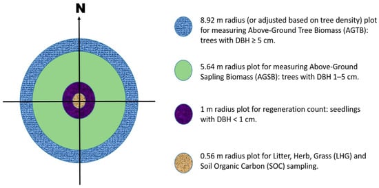 Figure 3. Sample plot layout.
3.1.3. Tree Measurements and Biomass Estimation
Tree diameters were measured using a diameter tape, and tree heights were estimated with an Abney level and linear tape, followed by trigonometric calculations. Understory vegetation, including grasses and herbs, was clipped and weighed in the field. Subsamples were dried in a laboratory oven at 102 °C for 24 h to determine oven-dry weight (Figure 4).
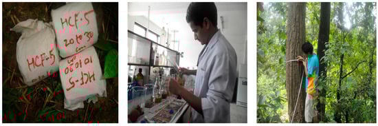
Figure 4.
Photographs of soil sample, lab work, DBH measurement (from left to right) for SOC and participatory ground inventory.
Appendix A, Table A3 describes plot-level environmental and site characteristics such as soil type, slope, vegetation cover, and disturbance indicators, which support the interpretation of field variability.
3.1.4. Biomass and Carbon Estimation
Reliable estimation of forest biomass is essential for understanding carbon dynamics and informing REDD+ initiatives. Several allometric models have been developed to estimate aboveground tree biomass (AGTB), varying in scope, applicability, and precision. Although Sharma proposed country-specific equations for Nepal [40], these models were derived from relatively small and geographically limited datasets, with restricted representation of tropical and subtropical forest types. Consequently, their applicability beyond specific ecological zones remains uncertain.
In contrast, the pan-tropical model by Chave is based on a large dataset encompassing diverse forest types and structural conditions across the tropics [41]. It incorporates tree height, diameter, and wood density, offering improved accuracy and broader transferability. This model is also widely validated, facilitates comparability with global carbon assessments, and is recommended for REDD+ and IPCC reporting frameworks. Hence, it was adopted in this study to ensure consistency and comparability with global biomass studies, while recognizing that further evaluation under Nepal-specific conditions could enhance local model calibration in future research.
The aboveground tree biomass (AGTB) was calculated using the allometric equation as follows [41]:
where,
- AGTB = above ground tree biomass (Kg)
- ρ = Wood specific gravity (Kg m−3)
- D = Tree diameter at breast height (m)
- H = Tree height (m)
We used the pan-tropical moist-forest equation [41], which incorporates DBH, total height, and wood density (ρ) and is widely recommended for REDD+ and IPCC Tier 2–3 carbon accounting. Species-level wood densities were obtained from the Global Wood Density Database and Nepal-specific publications (Appendix A). We also performed a sensitivity comparison using a Nepal-specific equation, e.g., Shorea robusta-based [42]. The resulting mean AGC differed by approximately 7%–10%, and relative differences among plots were conserved. This indicates that our key conclusions are robust to allometric model choice.
Stem biomass was multiplied by 0.45 and 0.11 to estimate branch and leaf biomass, respectively [43]. Biomass was converted to carbon by multiplying by 0.47 [44]. Sapling biomass was estimated using the regression model:
where
- AGSB = Above Ground Sapling Biomass (kg)
- a = intercept of allometric relationship for sapling (dimensionless)
- b = slope allometric relationship for sapling (dimensionless)
- D = Over bark diameter at breast height (measured at 1.3 m above the ground)
To ensure transparency and reproducibility, supplementary datasets are provided in the Appendix A. The allometric relationship and regression coefficients used for sapling biomass estimation are summarized in Table 1. Appendix A Table A1 presents the complete tree inventory data, including species-specific DBH, height, and wood density used for aboveground biomass estimation. These coefficients were derived from local species datasets to ensure appropriate biomass estimation for saplings. Carbon stock was again estimated using a 0.47 conversion factor [44]. Herbaceous vegetation and grasses within each sample plot were clipped at ground level and their total fresh weight (TFW) recorded in the field. A representative subsample of the clipped material was taken to obtain its sample fresh weight (SFW) and was subsequently oven-dried at 65 °C to a constant weight to determine the sample oven-dry weight (SODW). Because the entire plot sample was not oven-dried, the dry-to-fresh ratio of the subsample was used to estimate the total oven-dry weight (ODW):
where,

Table 1.
Allometric equation and regression coefficients used for sapling aboveground biomass estimation.
- ODW = Total oven dry weight
- TFW = Total fresh weight
- SODW = Sample oven dry weight
- SFW = Sample fresh weight
Carbon stock was estimated by applying the 0.47 factor [44]. The total aboveground carbon stock per hectare was computed by summing carbon contributions from tree biomass, saplings, herbs, and grasses:
where,
- TAGC = Total Above Ground Carbon [tC ha−1];
- C (AGTB) = Carbon stock in Aboveground Tree Biomass [tC ha−1];
- C (AGSB) = Carbon in Aboveground Sapling Biomass [tC ha−1];
- C (HG) = Carbon in Herbs and Grass [tC ha−1];
The result was converted to CO2 equivalents by multiplying by 3.67 [45].
3.2. Remote Sensing-Based Aboveground Carbon Assessment
3.2.1. Carbon Dataset Integration (2015–2022)
Satellite-derived aboveground biomass data for 2015–2022 were obtained from the Centre for Environmental Data Analysis (CEDA; Didcot, Oxfordshire, UK) using the European Space Agency’s (ESA; Paris, France) Climate Change Initiative (CCI) and GlobBiomass products. The GlobBiomass dataset provides global aboveground biomass estimates at 100 m resolution and is generated through the integration of ALOS PALSAR L-band synthetic aperture radar (SAR), Envisat ASAR C-band SAR, and Moderate Resolution Imaging Spectroradiometer (MODIS) optical data, combined with regional calibration using ground plots and allometric models. The CCI biomass product offers annual, harmonized AGB layers suitable for long-term carbon trend analysis. Both datasets were accessed through the CEDA archive (https://data.ceda.ac.uk/neodc/esacci/biomass/ accessed on 24 April 2025), and were used to assess temporal variations in aboveground forest carbon across the study area.
3.2.2. Time Series Analysis of Aboveground Forest Carbon
Raster datasets were reprojected to WGS 1984 UTM Zone 44N to ensure spatial consistency. Zonal statistics were computed using ArcGIS Desktop version 10.8 (Environmental Systems Research Institute—Esri, Redlands, CA, USA) to extract the mean aboveground biomass (AGB) per hectare within the Hariyali Community Forest. A biomass-to-carbon conversion factor of 0.47 was applied to estimate aboveground carbon stock per hectare [44], which was then scaled to the total forest area to calculate the total carbon stock for each year in the time series.
Field data were collected in 2022, while satellite biomass datasets span 2010–2022, enabling temporal trend analysis. We acknowledge this temporal mismatch and interpret trends accordingly, recognizing that field data offer fine-scale precision and satellite data provide valuable long-term monitoring.
3.3. Land Use and Land Cover (LULC) Analysis
3.3.1. LULC Data Acquisition (2000 and 2022)
Landsat 7 Enhanced Thematic Mapper Plus (ETM+) imagery (30 m resolution) from 2000 was acquired from the United States Geological Survey (USGS) Earth Explorer platform (USGS, Reston, VA, USA), while pre-classified LULC data for 2022 were obtained from the ArcGIS Living Atlas (Esri, Redlands, CA, USA). Atmospheric correction was applied to raw imagery, and cloud contamination and data gaps were masked and the bands were composited. The datasets were clipped to the study area and projected to WGS 1984 UTM Zone 44N for consistency. The 2000 LULC map was produced using supervised Maximum Likelihood Classification (MLC), while the 2022 map was obtained from the ESRI Global Land-Cover product. To ensure comparability, the 2022 classes were reclassified to match the 2000 schema. A validation using high-resolution satellite imagery yielded an overall accuracy of 93% and kappa = 0.89. We acknowledge methodological differences between years and discuss their implications for uncertainty and change detection.
3.3.2. Classification (Supervised Classification and Polygon Digitization) Validation
Supervised classification was performed on the 2000 Landsat imagery using the Maximum Likelihood Classification (MLC) algorithm in ArcGIS version 10.8 (Esri, Redlands, CA, USA). The satellite imagery for this classification was obtained from the United States Geological Survey (USGS; Reston, VA, USA). Training samples were collected based on a stratified random sampling strategy, and the classification was validated using ground truth points. Ground validation relied on satellite-derived high-resolution imagery from Google Earth Pro version 7.3 (Google LLC, Mountain View, CA, USA), community knowledge, and GPS-referenced field observations where available. For the remote sensing component, Appendix A, Table A4 provides the confusion matrix of the 2000 supervised land-cover classification, while Appendix A, Table A5 summarizes kappa value ranges and the corresponding strength of agreement used to evaluate classification accuracy. Manual polygon digitization was used to refine misclassified regions. Land use and land cover (LULC) categories included forest, shrubland, rangeland, water bodies, and built-up areas.
Classification accuracy was evaluated via a confusion matrix and kappa coefficient using 350 ground truth points from GPS-based field observations and high-resolution satellite imagery. The overall accuracy was 95%, with a kappa coefficient of 0.93, indicating reliable LULC classification for change detection analysis.
In contrast, the 2022 LULC dataset was sourced from ESRI’s Living Atlas of the World (Esri, Redlands, CA, USA), as a pre-classified, readily available land cover layer, requiring no additional supervised classification.
3.3.3. LULC Change Detection
A post-classification change detection approach was employed to compare the 2000 and 2022 classified maps. Change matrices were generated to quantify spatial and temporal transitions between LULC classes, with a focus on forest loss and gain. These changes were further analyzed for their spatial correlation with observed variations in aboveground carbon stock, allowing for interpretation of carbon dynamics in relation to land cover transformation.
Field-based carbon estimates, satellite-derived biomass data, and LULC change detection results were integrated to assess the spatiotemporal patterns of carbon dynamics in the Hariyali Community Forest. This multi-source triangulation enabled the cross-validation of remote sensing and field inventory data, thereby enhancing the reliability of the findings. By overlaying carbon trends with LULC transitions, the study provided insights into the impacts of land use change on carbon sequestration potential within this community-managed forest system.
4. Results
4.1. Tree Vegetation Characteristics
Six concentric circular permanent sample plots (250 m2 each) were established in the HCF, recording a total of 117 trees across seven species, with Sal (Shorea robusta) as the dominant species. Five DBH outlier trees with implausibly large or small diameter values caused by measurement or recording errors were excluded from the analysis. The DBH distribution followed a right-skewed trend, typical of regenerating forests with high recruitment and fewer mature individuals, indicating ongoing regeneration and strong potential for future carbon accumulation.
Plot-level and strata-wise averages were cross-validated to ensure consistency and representativeness of reported mean carbon densities. Tree density ranged from 160 trees/ha in sparse strata to 300 trees/ha in dense strata. However, higher tree density did not consistently translate into higher biomass or carbon stock due to the prevalence of smaller-diameter trees in some plots. Biomass variability also reflected species-specific differences in wood density.
The forest exhibited an inverted-J-shaped layer structure, characteristic of regenerating stands dominated by seedlings and saplings, with fewer mature individuals, suggesting a dynamic growth phase (Figure 5, Table 1). This structure supports the conclusion of sustained biomass growth over time.
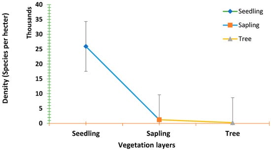
Figure 5.
Forest layer structure in Hariyali Community Forest.
The graph illustrates plant density across three forest layers: seedlings (~26,000/ha), saplings (~1000/ha), and mature trees (~100/ha). The steep density decline across layers reflects intense intra-species competition for light, nutrients, and space. Substantial variability in seedling density (as shown by error bars) highlights site-level differences in regeneration success. Native competition is the primary challenge, but the invasive species Lantana camara further suppress seedling survival by disrupting understory dynamics.
Regeneration assessments revealed the presence of diverse native species across all sampled plots (Appendix A, Table A2). Shorea robusta and Terminalia tomentosa were dominant, accompanied by species such as Lagerstroemia parviflora, Syzygium cumini, Terminalia chebula, and Phyllanthus emblica. The abundance of seedlings and saplings of both canopy and understory species indicates active natural regeneration and a stable successional trajectory within the community forest.
4.2. Vegetation Biomass
Field measurements across six 8.92 m radius plots yielded a mean aboveground carbon stock of 164.76 tC ha−1 (SE = 6.49; 95% CI: 149.55–181.05 tC ha−1), suggesting a relatively homogeneous carbon distribution across strata. Sapling biomass was higher in sparse forest strata (4.15 tC ha−1) than in dense strata (2.54 tC ha−1), likely due to increased light availability under open canopies.
Shrub biomass peaked in dense strata (4.68 tC ha−1) and was lowest in sparse areas (2.45 tC ha−1), suggesting favorable microclimatic conditions under moderate shading. Herbaceous biomass followed a similar trend, with higher values in dense strata (2.99 tC ha−1) versus sparse (2.56 tC ha−1). Combined, shrub and herbaceous biomass contributed approximately 1.8% and 0.8%, respectively, to the total aboveground carbon stock, highlighting the ecological significance of understory vegetation in multi-layered carbon storage.
4.3. Total Aboveground Carbon Stock Density
Table 2 presents the strata-wise total aboveground carbon stock. The majority of carbon was stored in trees, followed by shrubs, saplings, and herbaceous vegetation.
Table 2.
Strata- and Component-wise Aboveground Carbon Stock (tC ha−1).
Trees contributed the most to the total aboveground carbon stock, followed by shrubs, saplings, and herbaceous vegetation, respectively. Stratified analysis revealed slightly higher carbon density in dense strata (181.05 tC ha−1) compared to sparse strata (149.55 tC ha−1). This non-significant difference likely reflects the relatively young stand age and the uniform management history of the forest, both of which constrain biomass divergence despite apparent differences in canopy density. To ensure transparency and reproducibility, supplementary datasets are provided in the Appendix A. Appendix A, Table A1 presents the complete tree inventory data, including species-specific DBH, height, and wood density used for aboveground biomass estimation. A two-sample t-test comparing dense (181.05 tC ha−1) and sparse (149.55 tC ha−1) strata indicated no significant difference (t = 1.83, df = 4, p = 0.14). Cohen’s d = 1.00 suggests a moderate but non-significant effect, reflecting limited statistical power due to small sample size.
4.3.1. Satellite-Based Aboveground Biomass Carbon Trend (2010–2022)
Satellite-derived estimates indicate that aboveground carbon stock in HCF increased from 24.93 tC ha−1 in 2010 to a peak of 40.11 tC ha−1 in 2021, before slightly declining to 37.05 tC ha−1 in 2022 (Figure 6). This long-term trend clearly illustrates substantial carbon accumulation over the past decade, reflecting natural regeneration and sustained community stewardship.
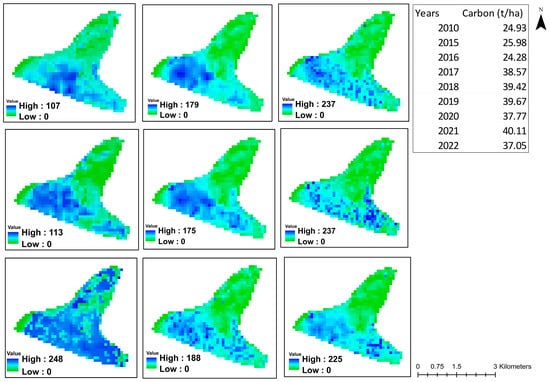
Figure 6.
Temporal Trends in Carbon Stock (2010–2022).
From 2010 to 2022, the carbon stock in the Hariyali Community Forest showed a general increasing trend, rising from 24.93 tC ha−1 in 2010 to 40.11 tC ha−1 in 2021. This steady growth reflects successful community stewardship and effective forest management interventions over time. However, a slight decline was observed between 2019 (39.67 tC ha−1) and 2020 (37.77 tC ha−1), followed by recovery in subsequent years. This short-term reduction appear to be associated with management activities implemented under the sustainable forest management (SFM) approach during that period. While detailed documentation is not available, it is understood that certain tree-thinning operations, intended to enhance stand structure and regeneration, may have been applied beyond their planned scope, temporarily reducing biomass density. The forest’s subsequent rebound in 2021 and 2022 indicates that the system quickly recovered under continued community oversight and adaptive management practices.
The moderate decline in 2022 compared to 2021 could be attributed to localized disturbances, selective harvesting, or short-term variability in vegetation productivity. Such fluctuations are common in remote sensing-derived products and should be interpreted within the broader positive trajectory. The overall net increase of ~12 tC ha−1 from 2010 to 2022 underscores the effectiveness of forest restoration and participatory management in enhancing ecosystem carbon storage.
4.3.2. Discrepancies Between Ground Measurements and Satellite-Derived Biomass
To provide a quantitative diagnostic of the discrepancy between field and satellite estimates, we compared the field-measured mean AGC for 2022 (164.76 tC ha−1; SE = 6.49; n = 6) with the satellite-derived estimate for the same year (37.05 tC ha−1). A one-sample t-test showed a significant difference (t = 19.68, df = 5, p ≪ 0.001). The effect size (Cohen’s d = 8.04) indicates a huge practical difference. The satellite value underestimated field AGC by 127.71 tC ha−1 (77.6%). This quantitative check confirms that coarse-resolution satellite biomass products substantially smooth or underestimate stand-level AGC in this community forest.
Recent studies consistently show that remote-sensing-derived biomass estimates diverge from ground-based inventories, especially in structurally complex tropical forests. For example, GEDI lidar observations have been shown to mis-estimate aboveground biomass when not calibrated with local field plots [46]. AGB estimation using Sentinel-2 data in tropical afro-montane forests similarly revealed significant uncertainty and systematic underestimation compared to field measurements [47]. Multi-source remote sensing approaches in tropical montane forests also reported persistent errors and limited agreement with ground-inventory biomass [48]. Even lidar-based assessments may substantially underpredict biomass in dense forests unless supported by ground calibration [49]. Regionally, lidar-referenced biomass maps in South Asia also demonstrate large mismatches when compared to coarse global biomass products, highlighting the need for site-specific calibration [50]. More recently, machine-learning models using GEDI and ICESat-2 canopy height retrievals show that significant bias remains unless ground data are incorporated [51]. A comprehensive review further confirms that remote-sensing biomass products frequently underperform relative to ground or airborne surveys, underscoring field measurements as the benchmark for accurate AGB estimation [52]. Collectively, these findings align with our observation that satellite-derived AGC (~37 tC ha−1) is substantially lower than field-derived AGC (165 tC ha−1), reflecting well-known limitations of uncalibrated remote sensing in dense, multi-layered tropical forests.
The maps were visualized using a standard deviation stretch, which enhances color contrast by representing pixel values relative to the mean (e.g., ±1 SD, ±2 SD), rather than showing the actual carbon quantities. Therefore, the SD-based color scale illustrates spatial variation and not absolute carbon values. It is important to note that satellite-based products operate at a relatively coarse spatial resolution (~100 m pixels), which tends to smooth fine-scale heterogeneity and underrepresent dense regeneration patches [53,54]. Consequently, while field-based inventories provide higher local accuracy, satellite data offer valuable temporal insights into decadal recovery dynamics. Integrating both approaches strengthens the reliability of carbon stock assessments.
Overall, the satellite-derived carbon trajectory, together with field measurements and LULC evidence, highlights a strong forest recovery pathway. Community-driven conservation, afforestation, and natural regeneration have collectively transformed the landscape, yielding significant carbon gains and reinforcing the role of participatory forest management in climate change mitigation.
4.4. LULC Change (2000–2022)
We used Landsat Collection 2 Level-2 surface reflectance data acquired from the United States Geological Survey (USGS) Earth Explorer portal. For the year 2000, imagery was obtained from the Landsat 7 Enhanced Thematic Mapper Plus (ETM+) sensor (C2 L2), and for 2022, imagery was obtained from the Landsat 8–9 Operational Land Imager/Thermal Infrared Sensor (OLI/TIRS) sensors (C2 L2). Both datasets provide atmospherically corrected surface reflectance products at a spatial resolution of 30 m across visible to shortwave infrared bands, and 15 m resolution for the panchromatic band. The thermal bands from OLI/TIRS are provided at 100 m resolution but resampled to 30 m. These Level-2 products include corrections for radiometric calibration, geometric alignment, and atmospheric effects (using the LaSRC algorithm for OLI/TIRS and LEDAPS for ETM+).
Land Use and Land Cover (LULC) analysis between 2000 and 2022 revealed a substantial expansion in woody vegetation cover, accompanied by a marked decline in rangeland areas (Figure 7). In 2000, woody vegetation cover occupied 449.10 ha (73.03%) of the total area, while rangelands extended over 165.78 ha (26.97%). By 2022, woody vegetation cover had expanded to 548.91 ha (89.27%), while rangeland declined sharply to 65.97 ha (10.73%). This represents a net gain of 99.81 ha of woody vegetation cover and a corresponding loss of 99.81 ha of rangeland over two decades, reflecting successful ecological recovery and vegetation regeneration.
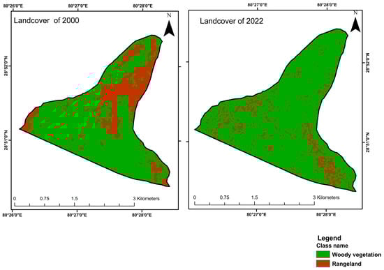
Figure 7.
LULC Area map 2000 and 2022.
The LULC maps (Figure 7) illustrate this transition, with large portions of rangeland in 2000 visibly converted into woody vegetation-dominated areas by 2022. These shifts are consistent with community-led restoration, natural regeneration, and improved forest stewardship practices that collectively drove positive landscape change.
In spite of previous concerns about temporal inconsistencies, the use of 2022 datasets for both LULC and carbon measurements ensures direct comparability. The observed expansion of woody vegetation cover in the GIS analysis strongly reinforces the carbon stock results derived from field inventory and remote sensing. Together, these findings demonstrate a clear positive relationship between forest recovery and carbon enhancement, highlighting the effectiveness of afforestation, natural regeneration, and community-led conservation in driving ecological transition within HCF.
These land-cover transitions, observed within a transboundary ecological corridor, mirror broader regional reforestation and agro-ecological recovery trends across South Asia, highlighting the cascading benefits of community-led forest governance on landscape resilience.
5. Discussion
Despite the limited number of field plots (n = 6), site selection was guided by pre-stratification using high-resolution satellite imagery and Google Earth Pro inspection, which indicated predominantly homogeneous forest canopy and terrain. The relatively flat topography and uniform vegetation cover, along with minimal variation in canopy texture or spectral reflectance, justified a more focused sampling strategy under logistical constraints. Stratification into dense and sparse canopy zones revealed only modest differences in carbon density (dense: 181.05 tC ha−1; sparse: 149.55 tC ha−1; CV ≈ 13.5%), suggesting low ecological heterogeneity. Such structural uniformity aligns with established patterns in community-managed Sal forests and supports the representativeness of the selected plots. The inventory used six plots (~0.05% sampling intensity), which is within the range applied in Nepal’s CFUG inventories for large community forests but may not capture fine-scale variation. Although our observed coefficient of variation (~13.5%) indicated moderate homogeneity, future inventories should increase plot numbers or integrate high-resolution remote sensing (UAV/LiDAR) to reduce uncertainty and improve spatial representation. Future studies could incorporate broader spatial sampling and UAV-assisted stratification to further validate these patterns.
Satellite biomass estimates (~37.05 tC ha−1) substantially underestimated carbon stocks compared to field measurements (165.30 tC ha−1) due to coarse spatial resolution and generalized allometric assumptions. Field inventories, which incorporate species-specific allometries, DBH, and wood density, capture fine-scale variability, highlighting the importance of integrating ground-truth data to calibrate remote sensing outputs. These discrepancies are expected and consistent with known limitations of coarse-resolution remote sensing, which often underestimates biomass in dense or vertically complex forests. Stratified analysis and structural observations confirm that field-based measurements more accurately reflect site-specific carbon storage, including understory contributions critical for future sequestration.
Evidence from Nepal supports this interpretation. Strong agreement was found between RS-based biomass (~209–214 t/ha) and field inventories (~210 t/ha) when LiDAR and satellite data were integrated [55]. Calibration with local plots improved LiDAR-based biomass predictions, reducing RMSE from ~106 to ~61 t/ha [56]. Landsat 8 imagery also underestimated biomass relative to field inventories in community forest buffer zones [57].
Global findings are consistent. RS estimates tend to diverge from ground data unless calibrated with field plots [58], and global biomass maps often over- or underestimate carbon unless combined with local observations [54]. Strong agreement between GEDI LiDAR and USFS plots was observed (R2 = 0.88–0.90), although biases persisted at density extremes [59]. Collectively, this evidence underscores the necessity of integrating local measurements with remote sensing to produce accurate carbon estimates.
The observed low coefficient of variation (CV ≈ 13.5%) further supports the structural and compositional homogeneity across strata. The J-shaped vertical profile and abundant regeneration layers reinforce the use of fewer plots for carbon estimation and emphasize the ecological value of multi-layered forest structure. The significant increase in tree cover (from 73.03% to 89.27%) and corresponding carbon gains highlight the critical role of community forests in climate mitigation, while temporary declines associated with Scientific Forest Management thinning reflect expected short-term reductions that promote long-term forest health. Balancing local livelihood needs with carbon objectives underscores the socio-ecological context of community forestry.
Combining field-based inventories with satellite remote sensing provides robust and actionable insights into forest carbon dynamics. The integration of ground truthing, structural assessments, and remote sensing ensures technical accuracy and informs adaptive management strategies. Our sampling intensity and number of plots (n = 6) align with national forest inventory protocols [34,35] and observed structural uniformity, consistently high regeneration, and low CV values support the representativeness of our estimates. Future research should expand sampling coverage, integrate UAV-based technologies, and apply bark correction factors to improve precision further.
Short-term AGC declines (2019–2020; 2021–2022) could be consistent with localized thinning under Scientific Forest Management, but without spatially explicit harvest records these should be interpreted as plausible hypotheses rather than definitive causal attributions. Broader policy implications (e.g., SDG/NDC contributions) are framed cautiously, as our findings represent a site-level case study rather than a generalizable national estimate. This study is subject to several limitations, including limited sampling intensity, height measurement error, lack of bark thickness correction, transfer uncertainty in allometric models, and remote-sensing resolution and temporal mismatches. These collectively contribute to uncertainty in AGC estimates and are acknowledged here to guide future improvements.
From a regional environmental change perspective, the observed carbon recovery trajectory reflects the capacity of community forestry to mediate coupled human–natural system dynamics under climate and land-use pressures. The convergence between remote sensing and field-based evidence demonstrates how participatory management can generate regionally significant climate mitigation outcomes while strengthening local adaptation capacity, contributing to national NDC targets and the 2030 Agenda for Sustainable Development, particularly in data-scarce mountainous regions.
6. Recommendations
Based on the findings of this study, the following evidence-driven recommendations are proposed to sustain and scale community forest carbon gains:
- 1.
- Establish Local Carbon Baselines and Monitoring:
Implement CFUG-level carbon inventories using the integrated field and satellite method. Institutionalize periodic re-measurement (every 3–5 years) to track gains (~12 tC ha−1 from 2010–2022) and support REDD+ reporting.
- 2.
- Science-Based Thinning and Regeneration Planning:
Guide thinning and regeneration using DBH distribution and regeneration density to sustain carbon gains and avoid temporary losses.
- 3.
- Multi-Layer Carbon Accounting:
Include saplings, shrubs, and herbaceous layers (~2.6 tC ha−1) in carbon reporting to better represent sequestration potential and enhance REDD+ payment accuracy.
- 4.
- Pilot Community Carbon Credit Schemes:
Leverage verified gains (~101,640 tC/373,017 tCO2e) to establish CFUG-led carbon trading frameworks, channeling revenues into forest regeneration and livelihoods.
- 5.
- Strengthen Adaptive Management:
Provide CFUG training in biomass monitoring, GIS mapping, and low-cost UAV or smartphone monitoring to reduce uncertainty and enhance management decisions.
- 6.
- Integrate Agroforestry Carbon in Buffer Zones:
Promote carbon-positive crops in buffer zones to enhance soil carbon and reduce pressure on core forests.
- 7.
- Policy Recognition of Community Forest Performance:
Formally recognize high-performing CFUGs in national carbon accounting and REDD+ benefit-sharing frameworks to incentivize sustained stewardship.
7. Conclusions
This study provides one of the first integrated assessments of aboveground carbon dynamics in a lowland Shorea robusta-dominated CFUG forest of Nepal, combining stratified field inventories with multi-temporal satellite-derived biomass and land-cover analyses. The convergence between field-measured (165 tC ha−1) and satellite-observed trends (net +12 tC ha−1 from 2010–2022) validates the reliability of integrated monitoring for community-managed forests. The J-shaped diameter structure, high regeneration density, and consistent carbon across strata indicate a stable and self-sustaining system with strong sequestration potential.
Two short-term carbon declines, first in 2019–2020 and again in 2021–2022, coincided with Scientific Forest Management (SFM) thinning and localized harvesting by the CFUG, illustrating how management intensity directly affects carbon outcomes. This underscores the need for adaptive, data-driven silviculture guided by continuous field-satellite monitoring. The demonstrated role of agroforestry mosaics in sustaining both carbon and livelihoods further highlights the importance of cross-scale land-use integration in carbon policy design.
This study highlights substantial differences between field-based and satellite-derived AGC estimates, underscoring the need for local calibration when applying coarse-resolution biomass products in community forests. While Hariyali CF demonstrates strong carbon stewardship, upscaling these findings requires expanded sampling, integration of UAV/LiDAR structural data, and harmonized LULC workflows. Future work should emphasize multi-temporal field measurements, refined allometric modeling, and locally calibrated remote-sensing approaches to enhance the reliability of REDD+ and community based MRV (Measurement Reporting and Verification).
Overall, this study highlights the crucial role of community-managed forests in mediating regional environmental change across South Asia’s forest–agriculture frontiers. By demonstrating measurable carbon accumulation, ecological recovery, and socio-economic co-benefits within a transboundary corridor, the research establishes a scalable model for integrating community forestry into regional adaptation and mitigation strategies. These insights reinforce the relevance of participatory forest management to achieving SDG 13 (Climate Action), SDG 15 (Life on Land), and SDG 1 (No Poverty), positioning Nepal’s community forests as both local livelihood systems and regional climate resilience mechanisms.
Author Contributions
Conceptualization, P.R.J., A.H. and B.K.M.; methodology, A.H. and P.R.J.; data curation, A.H., P.R.J. and A.S.M.; software, A.H.; validation, A.H., P.R.J. and B.K.M., investigation, A.H. and B.K.M.; writing—original draft preparation, P.R.J.; writing—review and editing, A.H., P.R.J. and A.S.M. All authors have read and agreed to the published version of the manuscript.
Funding
This research was funded by National Natural Science Foundation of China (Grant No. 42261144749, 42377158); National Foreign Expert Individual Human Project (Category H) (H20240400); International Science and Technology co-operation Program of Shaanxi Province (Grant No. 2024GH-ZDXM-24); and Shaanxi Provincial Agricultural science and technology 114 public welfare platform to serve rural revitalization practical technical training (Grant No. 2024NC-XCZX-06).
Institutional Review Board Statement
Not applicable.
Informed Consent Statement
Not applicable.
Data Availability Statement
The original contributions presented in the study are included in the article material; further inquiries can be directed to the corresponding author.
Acknowledgments
We acknowledge the dedication and collaboration of all authors in conducting this study and preparing the manuscript. We thank Nabin Raj Joshi for field monitoring, D.R. Ojha (forester), Kishor Joshi and Chitra Rawal for field support, and Ramesh Basnet (lab asst.) and SchEMS College, Kathmandu, for lab support.
Conflicts of Interest
The authors declare no conflicts of interest.
Appendix A
Table A1.
Plants’ Biomasses.
Table A1.
Plants’ Biomasses.
| Year | CFUG | Strata | Plot | Species | DBH (cm) | Wood Specific Density | Angle A | Angle B | Distance D | Tree Height | Tree Condition | AGTB (kg) | AGTB (ton) | TBA (m2) |
|---|---|---|---|---|---|---|---|---|---|---|---|---|---|---|
| 2022 | HCFUG | sparse | 1 | Ashaina | 240 | 0.95 | 65 | 0 | 15 | 33.56 | 86,585.44435 | 86.5854444 | 4.523893 | |
| 2022 | HCFUG | sparse | 1 | Saal | 150 | 0.88 | 63 | 0 | 10 | 21.12 | 21,285.1584 | 21.2851584 | 1.767146 | |
| 2022 | HCFUG | sparse | 1 | Saal | 155 | 0.88 | 47 | 0 | 12 | 14.36 | top cut | 15,453.19521 | 15.4531952 | 1.886919 |
| 2022 | HCFUG | sparse | 1 | Saal | 100 | 0.88 | 65 | 0 | 9 | 20.8 | 9316.736 | 9.316736 | 0.785398 | |
| 2022 | HCFUG | dense | 2 | Saal | 260 | 0.88 | 68 | 0 | 12 | 31.2 | 94,471.70304 | 94.471703 | 5.309292 | |
| 2022 | HCFUG | dense | 2 | Saal | 180 | 0.88 | 70 | 0 | 14 | 39.96 | 57,992.38157 | 57.9923816 | 2.54469 | |
| 2022 | HCFUG | dense | 2 | Saal | 190 | 0.88 | 73 | 0 | 12 | 40.75 | 65,892.3914 | 65.8923914 | 2.835287 | |
| 2022 | HCFUG | dense | 2 | Saal | 120 | 0.88 | 53 | 0 | 15 | 21.4 | 13,803.10272 | 13.8031027 | 1.130973 | |
| 2022 | HCFUG | dense | 2 | Saal | 118 | 0.88 | 59 | 0 | 14 | 24.75 | 15,436.17425 | 15.4361742 | 1.093588 | |
| 2022 | HCFUG | dense | 2 | Jamun | 151 | 0.88 | 45 | 0 | 14 | 15.5 | 15,830.18708 | 15.8301871 | 1.790786 | |
| 2022 | HCFUG | dense | 2 | Ashaina | 280 | 0.95 | 70 | 0 | 15 | 42.71 | 149,984.3995 | 149.984399 | 6.157522 | |
| 2022 | HCFUG | dense | 3 | Saal | 143 | 0.88 | 50 | 0 | 35 | 43.21 | 39,578.26898 | 39.578269 | 1.606061 | |
| 2022 | HCFUG | dense | 3 | Saal | 118 | 0.88 | 40 | 0 | 25 | 22.47 | 14,014.17517 | 14.0141752 | 1.093588 | |
| 2022 | HCFUG | dense | 3 | Saal | 160 | 0.88 | 60 | 0 | 12 | 20.78 | 23,827.91066 | 23.8279107 | 2.010619 | |
| 2022 | HCFUG | dense | 3 | Saal | 311 | 0.88 | 65 | 0 | 15 | 33.66 | 145,826.1279 | 145.826128 | 7.59645 | |
| 2022 | HCFUG | dense | 3 | Saal | 186 | 0.88 | 65 | 0 | 12 | 27.23 | 42,196.26239 | 42.1962624 | 2.717163 | |
| 2022 | HCFUG | dense | 3 | Ashaina | 360 | 0.95 | 62 | 0 | 20 | 39.11 | 227,035.2396 | 227.03524 | 10.17876 | |
| 2022 | HCFUG | dense | 3 | Saal | 122 | 0.88 | 60 | 0 | 20 | 36.14 | 24,093.96439 | 24.0939644 | 1.168987 | |
| 2022 | HCFUG | dense | 3 | Haldi | 370 | 0.64 | 52 | 0 | 35 | 44.79 | 274,653.3908 | 274.653391 | 10.7521 | |
| 2022 | HCFUG | dense | 3 | Saal | 270 | 0.88 | 62 | 0 | 16 | 31.59 | 103,151.9895 | 103.15199 | 5.725553 | |
| 2022 | HCFUG | dense | 3 | Saal | 145 | 0.88 | 63 | 0 | 14 | 28.97 | 27,282.54965 | 27.2825496 | 1.6513 | |
| 2022 | HCFUG | dense | 3 | Saal | 170 | 0.88 | 70 | 0 | 12 | 34.46 | 44,608.08405 | 44.608084 | 2.269801 | |
| 2022 | HCFUG | dense | 3 | Saal | 135 | 0.88 | 67 | 0 | 14 | 34.48 | 28,147.20322 | 28.1472032 | 1.431388 | |
| 2022 | HCFUG | dense | 3 | Saal | 218 | 0.88 | 55 | 0 | 20 | 30.06 | 63,988.57194 | 63.9885719 | 3.732526 | |
| 2022 | HCFUG | dense | 3 | Saal | 103 | 0.88 | 57 | 0 | 20 | 32.29 | 15,344.15401 | 15.344154 | 0.833229 | |
| 2022 | HCFUG | sparse | 4 | Saal | 165 | 0.88 | 66 | 0 | 17 | 39.68 | 48,388.2601 | 48.3882601 | 2.138246 | |
| 2022 | HCFUG | sparse | 4 | Saal | 224 | 0.88 | 67 | 0 | 18 | 43.9 | 98,664.52091 | 98.6645209 | 3.940814 | |
| 2022 | HCFUG | sparse | 4 | Saal | 118 | 0.88 | 60 | 0 | 17 | 30.84 | 19,234.40864 | 19.2344086 | 1.093588 | |
| 2022 | HCFUG | sparse | 4 | Ashaina | 318 | 0.95 | 60 | 0 | 20 | 36.14 | 163,697.8 | 163.6978 | 7.94226 | |
| 2022 | HCFUG | sparse | 4 | Jamun | 215 | 0.88 | 72 | 0 | 12 | 38.43 | 79,569.70699 | 79.569707 | 3.630503 | |
| 2022 | HCFUG | dense | 5 | Saal | 105 | 0.88 | 50 | 0 | 9 | 12.22 | leaning | 6034.624596 | 6.0346246 | 0.865901 |
| 2022 | HCFUG | dense | 5 | Saal | 146 | 0.88 | 60 | 0 | 8 | 15.35 | 14,655.96928 | 14.6559693 | 1.674155 | |
| 2022 | HCFUG | dense | 5 | Saal | 141 | 0.88 | 52 | 0 | 6 | 8.9 | 7925.536793 | 7.92553679 | 1.56145 | |
| 2022 | HCFUG | dense | 5 | Ashaina | 241 | 0.95 | 70 | 0 | 10 | 28.97 | 75,367.31348 | 75.3673135 | 4.561671 | |
| 2022 | HCFUG | dense | 5 | Saal | 204 | 0.88 | 58 | 0 | 22 | 36.7 | 68,411.1441 | 68.4111441 | 3.268513 | |
| 2022 | HCFUG | dense | 5 | Saal | 183 | 0.88 | 65 | 0 | 20 | 44.39 | 66,586.74399 | 66.586744 | 2.63022 | |
| 2022 | HCFUG | dense | 5 | Saal | 190 | 0.88 | 68 | 0 | 15 | 38.62 | 62,448.20014 | 62.4482001 | 2.835287 | |
| 2022 | HCFUG | dense | 6 | Saal | 121 | 0.88 | 45 | 0 | 10 | 11.5 | 7541.696228 | 7.54169623 | 1.149901 | |
| 2022 | HCFUG | dense | 6 | Saal | 158 | 0.88 | 60 | 0 | 15 | 26.48 | 29,609.60468 | 29.6096047 | 1.960668 | |
| 2022 | HCFUG | dense | 6 | Saal | 150 | 0.88 | 70 | 0 | 15 | 42.71 | 43,043.9922 | 43.0439922 | 1.767146 | |
| 2022 | HCFUG | dense | 6 | Kaflayo | 127 | 0.72 | 60 | 0 | 15 | 27.48 | 19,852.93062 | 19.8529306 | 1.266769 | |
| 2022 | HCFUG | dense | 6 | Saal | 90 | 0.88 | 52 | 0 | 10 | 14.28 | 5181.001056 | 5.18100106 | 0.636173 | |
| 2022 | HCFUG | dense | 6 | Tedu | 40 | 0.72 | 30 | 0 | 4.5 | 322.5024 | 0.3225024 | 0.125664 | ||
| 2022 | HCFUG | dense | 6 | Tedu | 90 | 0.72 | 40 | 0 | 6.5 | 2358.2988 | 2.3582988 | 0.636173 | ||
| 2022 | HCFUG | dense | 6 | Tedu | 50 | 0.72 | 45 | 0 | 5.8 | 649.484 | 0.649484 | 0.19635 |
Table A2.
List of Plant Regeneration.
Table A2.
List of Plant Regeneration.
| Year | District | Plot | Species | Total Numbers |
|---|---|---|---|---|
| 2022 | Kanchanpur | 1 | Saal (Shorea robusta) | 2 |
| Ashaina (Terminalia tomentosa, also known as Asna) | 1 | |||
| Gunauni (Melia azedarach or similar species). | 3 | |||
| Bayar (Ziziphus mauritiana) | 1 | |||
| kukath/dheda (Likely to be Lagerstroemia parviflora.) | 2 | |||
| Ruina (Lagerstroemia parviflora) | 1 | |||
| Harro (Terminalia chebula) | 1 | |||
| Barro (Terminalia bellirica) | 2 | |||
| Amala (Phyllanthus emblica or Emblica officinalis) | 1 | |||
| unknown (used to prepare alcohol) | 28 | |||
| 2022 | Kanchanpur | 2 | Tarul (Amorphophallus paeoniifolius) | 22 |
| Githa (Diploknema butyracea) | 18 | |||
| kukath/dheda (Woodfordia fruticosa) | 10 | |||
| Ruina (Terminalia bellirica ). | 4 | |||
| 2022 | Kanchanpur | 3 | Ruina (Lagerstroemia parviflora) | 15 |
| Raj brikshya (Cassia fistula) | 5 | |||
| Kukath/kopre (Morus alba) | 1 | |||
| Saal (Shorea robusta) | 2 | |||
| Malu (Ficus hispida) | 7 | |||
| Harro(Terminalia chebula) | 3 | |||
| Barro (Terminalia bellirica) | 2 | |||
| Amala (Phyllanthus emblica/Emblica officinalis) | 1 | |||
| 2022 | Kanchanpur | 4 | Tendu (Diospyros melanoxylon) | 1 |
| Ashna (Terminalia tomentosa/Terminalia elliptica) | 2 | |||
| Dehro (Lagerstroemia parviflora) | 1 | |||
| Kumo (Carpinus viminea) | 1 | |||
| Kaflayo (Myrica esculenta) | 1 | |||
| Jamun (Syzygium cumini) | 1 | |||
| Saal (Shorea robusta) | 1 | |||
| Harro (Terminalia chebula) | 2 | |||
| Barro (Terminalia bellirica) | 1 | |||
| Ruina (Lagerstroemia parviflora) | 1 | |||
| Bijaysaal (Pterocarpus marsupium) | 1 | |||
| Kusum (Schleichera oleosa) | 1 | |||
| Bhalayo (Semecarpus anacardium) | 2 | |||
| Kopri (Celtis australis or Grewia tiliaefolia) | 1 | |||
| Jangre (Melastoma malabathricum) | 1 | |||
| Rajbriksya/monkey stick (Cassia fistula) | 3 | |||
| 2022 | Kanchanpur | 5 | Tendu (Diospyros melanoxylon) | 1 |
| Saal (Shorea robusta) | 1 | |||
| Saaj (Terminalia tomentosa/Terminalia elliptica) | 1 | |||
| Copri (Holoptelea integrifolia) | 2 | |||
| Kaflayo (Myrica esculenta) | 1 | |||
| 2022 | Kanchanpur | 6 | Jamun (Syzygium cumini) | 1 |
| Saaj (Terminalia tomentosa/Terminalia elliptica) | 2 | |||
| Dudhi (Euphorbia hirta) | 1 |
Table A3.
Plot Description.
Table A3.
Plot Description.
| Plot | GPS X | GPS Y | Altitude (m) | Soil Type | Fire | Fodder | Grazing | Firewood | Timber | Encroachment | Wildlife | Soil Erosion | Vegetation Type | Slope | Soil Color | Soil Depth (cm) | Tree Crown | Shrub Cover | Grass Cover |
|---|---|---|---|---|---|---|---|---|---|---|---|---|---|---|---|---|---|---|---|
| 1 | 28°52′8.86″ N | 80°27′46.53″ E | 221 | sandy | 0 | 0 | 0 | 0 | 0 | 0 | 1 | 0 | 1 | 0 | gray | 15 | 45% | 25% | 25% |
| 2 | 28°50′58.01″ N | 80°27′27.62″ E | 240 | sandy | 0 | 0 | 0 | 0 | 0 | 0 | 1 | 0 | 1 | 0 | brown | 12 | 50% | 35% | 30% |
| 3 | 28°51′26.89″ N | 80°27′34.21″ E | 224 | sandy | 0 | 0 | 0 | 0 | 0 | 0 | 1 | 0 | 1 | 0 | brown | 15 | 35% | 40% | 30% |
| 4 | 28°51′37.85″ N | 80°27′53.36″ E | 249 | sandy | 0 | 0 | 0 | 0 | 0 | 0 | 1 | 0 | 1 | 0 | brown | 12 | 40% | 45% | 30% |
| 5 | 28°50′40.91″ N | 80°27′58.29″ E | 333 | sandy | 0 | 0 | 0 | 0 | 0 | 0 | 1 | 0 | 1 | 0 | brown | 12 | 45% | 50% | 35% |
| 6 | 28°51′16.36″ N | 80°26′50.32″ E | 340 | sandy | 0 | 0 | 0 | 0 | 0 | 0 | 1 | 0 | 1 | 0 | brown | 10 | 45% | 45% | 35% |
Table A4.
Confusion Matrix 2000 (supervised classification).
Table A4.
Confusion Matrix 2000 (supervised classification).
| ClassValue | C_1 | C_4 | C_7 | Total | U_Accuracy | Kappa |
|---|---|---|---|---|---|---|
| Trees | 100.00 | 1.00 | 1.00 | 102.00 | 0.98 | 0.00 |
| Shrubs and Bushes | 5.00 | 150.00 | 5.00 | 160.00 | 0.94 | 0.00 |
| Rangeland | 2.00 | 2.00 | 84.00 | 88.00 | 0.95 | 0.00 |
| Total | 107.00 | 153.00 | 90.00 | 350.00 | 0.00 | 0.00 |
| P_Accuracy | 0.93 | 0.98 | 0.93 | 0.00 | 0.95 | 0.00 |
| Kappa | 0.00 | 0.00 | 0.00 | 0.00 | 0.00 | 0.93 |
Table A5.
Level of Agreement with Kappa values.
Table A5.
Level of Agreement with Kappa values.
| S/N | Value Range of Kappa | Strength of Agreement | % of Reliability |
|---|---|---|---|
| 1. | k ≤ 0 | No agreement | 0%–4% |
| 2. | 0.01 ≤ k ≤ 0.20 | Fair | 5%–15% |
| 3. | 0.21 ≤ k ≤ 0.40 | Slight | 16%–35% |
| 4. | 0.41 ≤ k ≤ 0.60 | Moderate | 36%–63% |
| 5. | 0.61 ≤ k ≤ 0.80 | Substantial | 64%–81% |
| 6. | 0.81 ≤ k ≤ 1.00 | Almost perfect agreement | 82%–100% |
References
- Friedlingstein, P.; O’Sullivan, M.; Jones, M.W.; Andrew, R.M.; Gregor, L.; Hauck, J.; Le Quéré, C.; Luijkx, I.T.; Olsen, A.; Peters, G.P.; et al. Global Carbon Budget 2022. Earth Syst. Sci. Data 2022, 14, 4811–4900. [Google Scholar] [CrossRef]
- Smith, C.; Al Khourdajie, A.; Yang, P.; Folini, D. Climate uncertainty impacts on optimal mitigation pathways and social cost of carbon. Environ. Res. Lett. 2023, 18, 094024. [Google Scholar] [CrossRef]
- Pan, Y.; Birdsey, R.A.; Fang, J.; Houghton, R.; Kauppi, P.E.; Kurz, W.A.; Phillips, O.L.; Shvidenko, A.; Lewis, S.L.; Canadell, J.G.; et al. A Large and Persistent Carbon Sink in the World’s Forests. Science 2011, 333, 988–993. [Google Scholar] [CrossRef]
- Bastin, J.-F.; Finegold, Y.; Garcia, C.; Mollicone, D.; Rezende, M.; Routh, D.; Zohner, C.M.; Crowther, T.W. The global tree restoration potential. Science 2019, 365, 76–79. [Google Scholar] [CrossRef]
- Intergovernmental Panel on Climate Change (IPCC) (Ed.) Frontmatter. In Climate Change 2022—Mitigation of Climate Change: Working Group III Contribution to the Sixth Assessment Report of the Intergovernmental Panel on Climate Change; Cambridge University Press: Cambridge, UK, 2023; pp. i–ii. [Google Scholar] [CrossRef]
- Li, J.; Gao, L.; Hu, X.; Jia, J.; Wang, S. Effects of personal carbon trading scheme on consumers’ new energy vehicles replacement decision: An economic trade-off analysis. Environ. Impact Assess. Rev. 2023, 101, 107108. [Google Scholar] [CrossRef]
- Harris, N.L.; Gibbs, D.A.; Baccini, A.; Birdsey, R.A.; de Bruin, S.; Farina, M.; Fatoyinbo, L.; Hansen, M.C.; Herold, M.; Houghton, R.A.; et al. Global maps of twenty-first century forest carbon fluxes. Nat. Clim. Chang. 2021, 11, 234–240. [Google Scholar] [CrossRef]
- Nunes, C.A.; Berenguer, E.; França, F.; Ferreira, J.; Lees, A.C.; Louzada, J.; Sayer, E.J.; Solar, R.; Smith, C.C.; Aragão, L.E.O.C.; et al. Linking land-use and land-cover transitions to their ecological impact in the Amazon. Proc. Natl. Acad. Sci. USA 2022, 119, e2202310119. [Google Scholar] [CrossRef]
- Zhen, Y.; Zhang, X.; Zhang, C.; Gao, Q.; Dong, J.; Zhang, L.; Lu, X.; Wang, Y. Effects of climate change and land use/cover changes on carbon sequestration in forest ecosystems in the coastal area of China. Front. For. Glob. Chang. 2023, 6, 1271239. [Google Scholar] [CrossRef]
- Joshi, P.R.; Huo, A.; Rijal, M. Impact of Land-Use Changes on Carbon Sequestration and Economic Losses: Insights from the Northern Qinling Mountains, China. J. Sustain. For. 2025, 1–29. [Google Scholar] [CrossRef]
- Bhusal, N. Avian Diversity and Abundance in the Machhaplan Complex, Hetauda, Nepal. For. J. Inst. For. Nepal 2021, 18, 90–106. [Google Scholar] [CrossRef]
- Lamsal, P.; Aryal, K.R.; Adhikari, H.; Paudel, G.; Maharjan, S.K.; Khatri, D.J.; Sharma, R.P. Effects of Forest Management Approach on Carbon Stock and Plant Diversity: A Case Study from Karnali Province, Nepal. Land 2023, 12, 1233. [Google Scholar] [CrossRef]
- Uprety, D.R.; Gurung, A.; Bista, R.; Karki, R.; Bhandari, K. Community Forestry in Nepal:A Scenario of Exclusiveness and its Implications. Front. Sci. 2012, 2, 41–46. [Google Scholar] [CrossRef]
- Dhungana, N.; Lee, C.-H.; Khadka, C.; Adhikari, S.; Pudasaini, N.; Ghimire, P. Evaluating Community Forest User Groups (CFUGs)’ Performance in Managing Community Forests: A Case Study in Central Nepal. Sustainability 2024, 16, 4471. [Google Scholar] [CrossRef]
- Aase, T.H.; Chapagain, P.S. Changing forest coverage and understanding of deforestation in Nepal Himalayas. Geogr. J. Nepal 2020, 13, 1–28. [Google Scholar] [CrossRef]
- FAO. Global Forest Resources Assessment 2020, Main Report; FAO: Rome, Italy, 2020. [Google Scholar] [CrossRef]
- FAO. Global Forest Resources Assessment and Remote Sensing Survey; FAO: Rome, Italy, 2022. [Google Scholar] [CrossRef]
- FRTC. Churia Forests of Nepal 2022; Ministry of Forests and Environment: Kathmandu, Nepal, 2022.
- Banskota, K.; Karky, B.; Skutsch, M. Reducing Carbon Emissions Through Community-Managed Forests in the Himalaya; International Centre for Integrated Mountain Development: Lalitpur, Nepal, 2007. [Google Scholar] [CrossRef]
- FAO. The State of Food and Agriculture 2021; FAO: Rome, Italy, 2021. [Google Scholar] [CrossRef]
- Chapagain, D.; Bharati, L.; Mechler, R.; Samir, K.C.; Pflug, G.; Borgemeister, C. Understanding the role of climate change in disaster mortality: Empirical evidence from Nepal. Clim. Risk Manag. 2024, 46, 100669. [Google Scholar] [CrossRef]
- Beyene, A.D.; Bluffstone, R.; Mekonnen, A. Community forests, carbon sequestration and REDD+: Evidence from Ethiopia. Environ. Dev. Econ. 2016, 21, 249–272. [Google Scholar] [CrossRef]
- Ulvdal, P. Stand Dynamics and Carbon Stock in a Sal (Shorea robusta C.F. Gaertn) Dominated Forest in Southern Nepal. Master’s Thesis, Swedish University of Agricultural Sciences, Uppsala, Sweden, 2016. [Google Scholar]
- Bhattarai, T.; Skutsch, M.M.; Midmore, D.; Rana, E. The Carbon Sequestration Potential of Community-based Forest Management in Nepal. Int. J. Clim. Chang. Impacts Responses 2012, 3, 233–253. [Google Scholar] [CrossRef]
- Sapkota, I.; Tigabu, M.; Odé, C. Spatial distribution, advanced regeneration and stand structure of Nepalese Sal (Shorea robusta) forests subject to disturbances of different intensities. For. Ecol. Manag. 2009, 257, 1966–1975. [Google Scholar] [CrossRef]
- Staddon, S. Carbon Financing and Community Forestry: A Review of the Questions, Challenges and the Case of Nepal. J. For. Livelihood 2009, 8, 25–32. [Google Scholar]
- Çelik, D.A.; Altunel, A.O. Is Dynamic World a Contender in Global Land-Cover Making Race? A Swift Field Assessment from Kastamonu, Türkiye. Egypt. J. Remote Sens. Space Sci. 2025, 28, 205–213. [Google Scholar] [CrossRef]
- Celik, D.A.; Şahin, A. Spatiotemporal changes of carbon storage in Çaltepe Forest Planning Unit. Artvin Çoruh Üniv. Orman Fak. Derg. 2023, 24, 224–233. [Google Scholar] [CrossRef]
- Bhatta, S.P.; Devkota, A. Carbon stock in the community managed Sal (Shorea robusta) forests of Dadeldhura district, western Nepal. South. For. A J. For. Sci. 2020, 82, 47–55. [Google Scholar] [CrossRef]
- Ayer, K.; Kandel, P.; Gautam, D.; Khadka, P.; Sayab Miya, M. Comparative Study of Carbon Stock and Tree Diversity between Scientifically and Conventionally Managed Community Forests of Kanchanpur District, Nepal: 10.32526/ennrj/20/202200010. Environ. Nat. Resour. J. 2022, 20, 494–504. [Google Scholar] [CrossRef]
- Smith, A.C.; Hurni, K.; Fox, J.; Van Den Hoek, J. Community forest management led to rapid local forest gain in Nepal: A 29 year mixed methods retrospective case study. Land Use Policy 2023, 126, 106526. [Google Scholar] [CrossRef]
- Tripathi, S.; Subedi, R.; Adhikari, H. Forest Cover Change Pattern after the Intervention of Community Forestry Management System in the Mid-Hill of Nepal: A Case Study. Remote Sens. 2020, 12, 2756. [Google Scholar] [CrossRef]
- NSO. National Population and Housing Census 2021; NSO: Kathmandu, Nepal, 2021. [Google Scholar]
- Ojha, H. Department of Forest’s new community Forestry Guideline. J. For. Livelihood 2024, 2, 78–81. [Google Scholar] [CrossRef]
- Luintel, H.; Bluffstone, R.A.; Scheller, R.M. The effects of the Nepal community forestry program on biodiversity conservation and carbon storage. PLoS ONE 2018, 13, e0199526. [Google Scholar] [CrossRef] [PubMed]
- Rana, E.B.; Shrestha, H.L.; Silwal, R. Participatory Carbon Estimation in Community Forest: Methodologies and Learnings. Initiation 2008, 2, 91–98. [Google Scholar] [CrossRef]
- Regmi, S.; Dahal, K.P.; Sharma, G.; Regmi, S.; Miya, M.S. Biomass and Carbon Stock in the Sal (Shorea robusta) Forest of Dang District Nepal. Indones. J. Soc. Environ. Issues (IJSEI) 2021, 2, 204–212. [Google Scholar] [CrossRef]
- Baral, S.K.; Malla, R.; Ranabhat, S. Above-ground carbon stock assessment in different forest types of Nepal. Banko Janakari 2010, 19, 10–14. [Google Scholar] [CrossRef]
- Khanal, S.; Boer, M.M. Plot-level estimates of aboveground biomass and soil organic carbon stocks from Nepal’s forest inventory. Sci. Data 2023, 10, 406. [Google Scholar] [CrossRef]
- Sharma, C.M.; Pukkala, T. Biomass Equations for Terai Forests of Nepal; Forest Survey and Statistics Division: Kathmandu, Nepal, 1990.
- Chave, J.; Andalo, C.; Brown, S.; Cairns, M.A.; Chambers, J.Q.; Eamus, D.; Fölster, H.; Fromard, F.; Higuchi, N.; Kira, T.; et al. Tree allometry and improved estimation of carbon stocks and balance in tropical forests. Oecologia 2005, 145, 87–99. [Google Scholar] [CrossRef]
- Pukkala, T. A Guide to Biomass Modelling for Forest Inventory in Nepal; Forest Survey and Statistic Division: Kathmandu, Nepal, 1990.
- Sharma, R.P.; Vacek, Z.; Vacek, S. Individual tree crown width models for Norway spruce and European beech in Czech Republic. For. Ecol. Manag. 2016, 366, 208–220. [Google Scholar] [CrossRef]
- IPCC. 2006 IPCC Guidelines for National Greenhouse Gas Inventories. Volume 4: Agriculture, Forestry and Other Land Use, Chapter 4: Forest Land; Institute for Global Environmental Strategies (IGES): Hayama, Japan, 2006. [Google Scholar]
- Pearson, T.R.H.; Brown, S.L.; Birdsey, R.A. Measurement Guidelines for the Sequestration of Forest Carbon; U.S. Department of Agriculture, Forest Service, Northern Research Station: Madison, WI, USA, 2007. [CrossRef]
- Sun, M.; Cui, L.; Park, J.; García, M.; Zhou, Y.; Silva, C.A.; He, L.; Zhang, H.; Zhao, K. Evaluation of NASA’s GEDI Lidar Observations for Estimating Biomass in Temperate and Tropical Forests. Forests 2022, 13, 1686. [Google Scholar] [CrossRef]
- Muhe, S.; Argaw, M. Estimation of above-ground biomass in tropical afro-montane forest using Sentinel-2 derived indices. Environ. Syst. Res. 2022, 11, 5. [Google Scholar] [CrossRef]
- Madundo, S.D.; Mauya, E.W.; Kilawe, C.J. Comparison of multi-source remote sensing data for estimating and mapping above-ground biomass in the West Usambara tropical montane forests. Sci. Afr. 2023, 21, e01763. [Google Scholar] [CrossRef]
- Sillett, S.C.; Graham, M.E.; Montague, J.P.; Antoine, M.E.; Koch, G.W. Ground-based calibration for remote sensing of biomass in the tallest forests. For. Ecol. Manag. 2024, 561, 121879. [Google Scholar] [CrossRef]
- Rodda, S.R.; Fararoda, R.; Gopalakrishnan, R.; Jha, N.; Réjou-Méchain, M.; Couteron, P.; Barbier, N.; Alfonso, A.; Bako, O.; Bassama, P.; et al. LiDAR-based reference aboveground biomass maps for tropical forests of South Asia and Central Africa. Sci. Data 2024, 11, 334. [Google Scholar] [CrossRef]
- Zhang, B.; Wang, Z.; Ma, T.; Wang, Z.; Li, H.; Ji, W.; He, M.; Jiao, A.; Feng, Z. Correcting forest aboveground biomass biases by incorporating independent canopy height retrieval with conventional machine learning models using GEDI and ICESat-2 data. Ecol. Inform. 2025, 86, 103045. [Google Scholar] [CrossRef]
- Kemigyisha, F.; Naturinda, E.; Omia, E.; Aboth, J.; Mutiibwa, D.; Kabenge, I.; Gidudu, A.; Kiggundu, N. Quantifying forest above ground biomass: A critical review of methods, challenges, and opportunities. Trees For. People 2025, 22, 101057. [Google Scholar] [CrossRef]
- Gibbs, H.; Brown, S.; Niles, J.; Foley, J. Monitoring and estimating tropical forest carbon stocks: Making REDD a reality. Environ. Res. Lett. 2007, 2, 045023. [Google Scholar] [CrossRef]
- Avitabile, V.; Herold, M.; Heuvelink, G.B.M.; Lewis, S.L.; Phillips, O.L.; Asner, G.P.; Armston, J.; Ashton, P.S.; Banin, L.; Bayol, N.; et al. An integrated pan-tropical biomass map using multiple reference datasets. Glob. Change Biol. 2016, 22, 1406–1420. [Google Scholar] [CrossRef]
- Kandel, P.N. Estimation of Above Ground Forest Biomass and Carbon Stock by Integrating Lidar, Satellite Image and Field Measurement in Nepal. J. Nat. Hist. Mus. 2015, 28, 160–170. [Google Scholar] [CrossRef]
- Kc, Y.B.; Liu, Q.; Saud, P.; Gaire, D.; Adhikari, H. Estimation of Above-Ground Forest Biomass in Nepal by the Use of Airborne LiDAR, and Forest Inventory Data. Land 2024, 13, 213. [Google Scholar] [CrossRef]
- Pandit, S.; Tsuyuki, S.; Dube, T. Landscape-Scale Aboveground Biomass Estimation in Buffer Zone Community Forests of Central Nepal: Coupling In Situ Measurements with Landsat 8 Satellite Data. Remote Sens. 2018, 10, 1848. [Google Scholar] [CrossRef]
- Goetz, S.J.; Baccini, A.; Laporte, N.T.; Johns, T.; Walker, W.; Kellndorfer, J.; Houghton, R.A.; Sun, M. Mapping and monitoring carbon stocks with satellite observations: A comparison of methods. Carbon Balance Manag. 2009, 4, 2. [Google Scholar] [CrossRef] [PubMed]
- Potapov, P.; Li, X.; Hernandez-Serna, A.; Tyukavina, A.; Hansen, M.C.; Kommareddy, A.; Pickens, A.; Turubanova, S.; Tang, H.; Silva, C.E.; et al. Mapping global forest canopy height through integration of GEDI and Landsat data. Remote Sens. Environ. 2021, 253, 112165. [Google Scholar] [CrossRef]
Disclaimer/Publisher’s Note: The statements, opinions and data contained in all publications are solely those of the individual author(s) and contributor(s) and not of MDPI and/or the editor(s). MDPI and/or the editor(s) disclaim responsibility for any injury to people or property resulting from any ideas, methods, instructions or products referred to in the content. |
© 2025 by the authors. Licensee MDPI, Basel, Switzerland. This article is an open access article distributed under the terms and conditions of the Creative Commons Attribution (CC BY) license (https://creativecommons.org/licenses/by/4.0/).