Abstract
North America’s midcontinent forest–prairie ecotone is currently exhibiting extensive eastern redcedar (ERC) (Juniperus virginiana L.) encroachment. Rapid expansion of ERC has major impacts on the species composition and forest structure within this region and suppresses previously dominant oak (Quercus) species. In Kansas, the growing-stock volume of ERC increased by 15,000% during 1965–2010. The overarching goal of this study was to evaluate the spatio-temporal dynamics of ERC in the forest–prairie ecotone of Kansas and understand its effects on deciduous forests. This was achieved through two specific objectives: (i) characterize an effective image classification approach to map ERC expansion, and (ii) assess ERC expansion between 1986 and 2017 in three study areas within the forest–prairie ecotone of Kansas, and especially expansion into deciduous forests. The analysis was based on satellite imagery acquired by Landsat TM and OLI sensors during 1986–2017. The use of multi-seasonal layer-stacks with a Support Vector Machine (SVM)-supervised classification was found to be the most effective approach to classify ERC distribution with high accuracy. The overall accuracies for the change maps generated for the three study areas ranged between 0.95 (95 CI: ±0.02) and 0.96 (±0.03). The total ERC cover increased in excess of 6000 acres in each study area during the 30-year period. The estimated percent increase of ERC cover was 139%, 539%, and 283% for the Tuttle Creek reservoir, Perry reservoir, and Bourbon County north study areas, respectively. This astounding rate of expansion had significant impacts on the deciduous forests where the conversion of deciduous woodlands to ERC, as a percentage of the total encroachment, were 48%, 56%, and 71%, for the Tuttle Creek reservoir, Perry reservoir, and Bourbon County north study areas, respectively. These results strongly affirm that control measures should be implemented immediately to restore the threatened deciduous woodlands of the region.
1. Introduction
Vegetation communities in ecotones are vulnerable to alterations in species composition due to the combined effects of climate change and land management practices since they are close to the limits of their natural ranges [1]. Within the schema of ecoregion classification for the United States [2], the transitional region between the heavily forested eastern US and the prairie grasslands of the Midwest is identified as the forest–prairie transitional region [3]. This midcontinent forest–prairie transitional region/ecotone of North America is currently experiencing extensive eastern redcedar (Juniperus virginiana) encroachment into the prairie ecosystem [4,5]. Eastern redcedar (ERC) continues to expand in area and density, particularly in Missouri, Nebraska, Kansas, and Oklahoma. Simultaneously, it drives major alterations in species composition and forest structure in this region, suppressing the dominant oak (Quercus) species [1,6].
In Kansas, the Forest Inventory and Analysis (FIA) data suggest that the growing-stock volume of ERC increased by 15,000% between 1965 and 2010 [7]. Kansas only has 2.4 million acres of forest land remaining, which constitutes just 5% of the state’s total land base. Because forests make up such a small area of the state, they play an important role in providing habitats for wildlife and delivering many other ecological, economic, and aesthetic benefits to the state. Oak/hickory is the predominant forest-type group in Kansas, accounting for 55% of the total forest lands [7]. Continued fire suppression in forestlands and the adverse effects of climate change, such as prolonged drought, would continue the current trend of shifting Quercus-dominated forests to Juniperus-dominated forests in this region and adversely affect associated ecosystem services [1]. Further, conversion of oak forests to ERC will intensify ERC expansion into the neighboring grasslands [6].
Identifying locations where ERC expansion is occurring at rapid rates is essential for land managers to plan and manage control efforts [6], such as using prescribed fire treatments and mechanical thinning [8]. Although ERC encroachment into the prairie ecosystem of the central US has been documented extensively [4,9,10], the threat of ERC in driving a structural and species compositional change in deciduous forests is less commonly studied. Available literature on ERC expansion in the forest–prairie ecotone of Kansas has been focused on grasslands, and no multi-temporal study has been conducted on the effects of ERC expansion on the remaining woodlands of Kansas. Conducting a spatial analysis to “identify locations where proactive management will be most effective” has been identified as one of the research priorities for the control of ERC expansion in this region [11]. Therefore, a remote sensing-based approach was utilized to conduct a multi-temporal change detection study to investigate ERC expansion, with two specific objectives: (i) Characterizing an effective classification approach to map ERC expansion, by assessing different classification algorithms and Landsat image preparation schemes; and (ii) assess ERC expansion between 1986 and 2017 in three study areas within the forest–prairie ecotone of Kansas, as well as its effects on the deciduous forests. The three study areas used in this analysis were selected based on the current ERC distribution. With the abundant ERC distribution found in these locations, it enabled the analysis to go back in time and characterize expansion rates within the last 30 years using archival Landsat satellite imagery.
2. Materials and Methods
Analysis of remote sensing imagery provides a powerful analytical tool for investigating vegetation dynamics and landcover change detection [12,13,14,15]. However, accurate image classification can be challenging. Due to the large size of data files, high dimensionality, and complexity, computationally efficient data mining algorithms and techniques are required to accurately convert these data into meaningful thematic information [16,17]. There are various pattern recognition or data mining techniques available for remote sensing image classification. Therefore, the user needs to select the most effective data mining technique for accurate image classification.
Being an evergreen tree species, ERC remains relatively constant in spectral characteristics throughout the year. Therefore, imagery acquired in the dormant season can be used to extract the ERC cover type from deciduous forests with high accuracy [18]. By utilizing a time series of cloud-free, dormant-season Landsat images spanning 2–3 decades, “gradual ecosystem changes” [19] could be characterized. However, appropriate image processing techniques should be used prior to analysis.
2.1. Study Areas and Datasets Used
To identify areas with a high ERC distribution within the forest–prairie ecotone of Kansas, three cloud-free Landsat OLI images, namely scene path 28/row 33 (21 January 2017), path 27/row 33 (3 March 2017), and path 27/row 34 (3 March 2017), were downloaded from the United States Geological Survey EarthExplorer website (http://earthexplorer.usgs.gov). These three Landsat scenes cover most of the forest–prairie ecotone of Kansas (Figure 1).
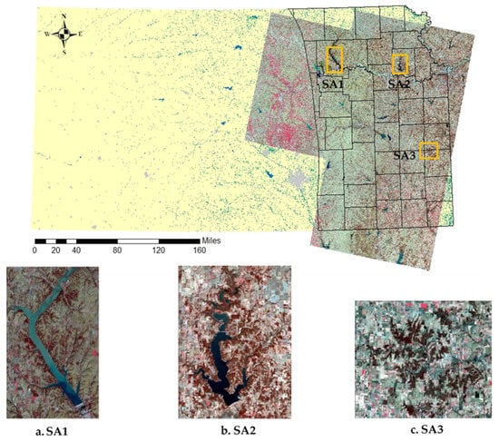
Figure 1.
Selection of the three study areas: (a) SA1—Tuttle Creek reservoir, (b) SA2—Perry reservoir, and (c) SA3—Bourbon County North. Three Landsat OLI images, namely scene path 28/row 33, path 27/row 33, and path 27/row 34 covers the majority of the forest–prairie ecotone of Kansas, outlined in black in the Kansas county map.
The images were selected from the dormant season for an accurate identification of the ERC cover type, as it is the most abundant evergreen tree species in the region. Images were displayed in a false-color scheme: near infra-red (NIR), red, and green. The mosaiced image was visually examined to identify areas with a wide ERC distribution. After careful inspection based on local knowledge of vegetation cover classes (information gathered through discussions with a group of subject matter experts with expertise in forest and range management, research, and extension), three study areas were selected: (i) Study Area 1 (SA1)—surrounding Tuttle Creek reservoir; (ii) Study Area 2 (SA2)—surrounding Perry reservoir; and (iii) Study Area 3 (SA3)—Bourbon county north (Figure 1).
Twelve cloud-free, Landsat Level-2 surface reflectance products were obtained through the USGS EarthExplorer website (Table 1).

Table 1.
Landsat scenes used in the study.
Images obtained for the time period of 1986–1988 were acquired by the Landsat-5 Thematic Mapper (TM) sensor, while the recent imagery for 2015–2017 were acquired by the Landsat-8 Operational Land Imager (OLI) sensor. There are major differences between the sensors and image products. However, the 30-m spatial resolution remains the same for the spectral bands used in this study. The Level-2 surface reflectance products were atmospherically corrected, which were generated from Landsat Ecosystem Disturbance Adaptive Processing System (LEDAPS) for Landsat TM images, and Landsat Surface Reflectance Code (LaSRC) for Landsat OLI images. This processing ensures higher consistency and comparability between images taken at different time periods compared to Level-1 digital number imagery [20,21]. Thus, it eliminates the requirement for additional pre-processing.
2.2. Assessment of Classification Algorithms
The dominant land cover classes in all these three selected areas were water, wetland areas, grasslands, crop fields, deciduous woodlands, and ERC forests. None of the areas contained major cities, and all other urban features, including roads and residential areas, were hardly discernible in the 30-m medium-resolution imagery. Hence, the urban land cover class was ignored in the analysis.
The study area surrounding the Tuttle Creek reservoir (SA1) was used to assess different classification approaches. Initially, four classification algorithms, namely the k-means clustering, Iterative Self-Organizing Data Analysis Technique (ISODATA), maximum likelihood (MLC), and support vector machines (SVM), were evaluated based on their classification accuracies of two single-date Landsat layer stacks for SA1. Each classification approach was expected to classify the two images with six land cover classes: water, grasslands, ERC, crop fields, wetlands, and deciduous woodlands. Image classification was performed using ENVI 5.3 software.
2.2.1. K-Means Clustering Algorithm
K-means clustering is an unsupervised classification technique. The end goal of the k-means algorithm is to find the optimal division of n entities in k groups. First, the algorithm must determine the initial number of clusters present in the data, and then locate the cluster means within the feature space. Within the process, each pixel is associated with the nearest cluster center using the Euclidean distance [22,23]. Based on the allocated pixels, the cluster means are re-calculated. This migration of cluster means is done iteratively until an optimal solution is reached where cluster means no longer change or the change from one iteration to another is less than a pre-defined threshold [22]. This iterative process reaches a cluster solution with high intra-class similarity and low inter-class similarity, and each data point can only be in one cluster.
After investigating for different combinations, the maximum number of classes and iterations were set to 10 and 20 respectively, which produced a reasonable classification result for the major cover classes. The classified images were manually inspected against the original Landsat image and an image with a higher resolution.
Google Earth TM (http://earth.google.com) images and National Agriculture Image Program (NAIP) imagery were downloaded though the USDA geospatial data gateway (https://datagateway.nrcs.usda.gov), and were used to inspect the 1986 and 2017 images along with the original Landsat images. Each of the ten classes were assigned to one of the six land cover classes mentioned earlier, to generate the final classified images (Figure 2c,d).
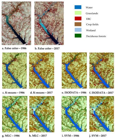
Figure 2.
False color composite of the study area surrounding the Tuttle Creek reservoir (SA1) in (a) 1986 and (b) 2017. K-means clustering classification products: (c) 1986 and (d) 2017. ISODATA clustering classification products: (e) 1986 and (f) 2017. Maximum Likelihood classification products: (g) 1986 and (h) 2017. Support Vector Machines (SVM) classification products: (i) 1986 and (j) 2017.
2.2.2. ISODATA
ISODATA is another unsupervised clustering algorithm used for land-use and landcover change detection [24,25], which is similar in most ways to the k-means clustering algorithm. In both k-means clustering and ISODATA, the objective is to minimize the mean squared distance from each data point to its nearest centroid (cluster center). However, the significant advantage of ISODATA over the k-means method is its ability to alter the number of clusters by deleting small clusters, merging nearby clusters, or splitting large diffuse clusters without user intervention [26]. The same sequence of steps as in the k-means clustering technique was employed using the ISODATA unsupervised classification tool of ENVI. The maximum number of classes was set to 10 with a minimum of 5. The change threshold was set at 5% and the minimum pixels per class to 1000. The initial clustering output generated 10 clusters, and these cluster were combined appropriately to generate the final classified images (Figure 2e,f).
2.2.3. Maximum Likelihood Classification (MLC)
In contrast to the unsupervised classification, supervised classification requires the user to select “training areas” for each pre-defined information class, which are used for statistical assessment of class reflectance, which is then extrapolated to the whole image [22,27]. Classification accuracy of this approach is highly dependent on how well the user defines these training areas. The training dataset is used to estimate the parameters of the classifier, and how well these parameter estimations are done will influence the overall accuracy of the final image classification [28]. Since selection of accurate training sites is crucial, the analyst should be extremely knowledgeable about the area. Though selection of training sites is a tedious task, supervised classification is still preferred over unsupervised methods since it gives more accurate class definitions and high classification accuracy [22].
MLC is one of the most commonly used parametric classifiers in change detection studies [29]. In MLC, the probability of each pixel belonging to one of each pre-defined set of classes is calculated using the mean and variance of each training class. This will create contours of probabilities around means of training data classes, and the unknown pixel will be placed in the most probable class based on the contours [22]. Since this classification is based on the mean and variance of the training sample, the training data sample should be large enough to represent the variance of that class throughout the image. The pre-defined training areas were selected to train the algorithm and to conduct the classification (Figure 2g,h).
2.2.4. Support Vector Machines (SVMs)
Support Vector Machines (SVMs) is a supervised non-parametric learning technique [30,31]. It represents a group of theoretically superior machine learning algorithms which locates the optimal boundaries between classes in a feature space [32,33]. In its simplest form, SVMs are linear binary classifiers which classify observations into one of the two possible labels by defining the optimal boundary between the two classes. At three dimensions this boundary becomes a plane, and with an increasing number of variable dimensions, the separator becomes a hyperplane. The SVM classification tool in ENVI was used to perform the classification. To approach an effective hyperplane, we chose the radial basis function (RBF, a Gaussian kernel) as the kernel type, considering that RBF allows for a nonlinear transformation of the training dataset. This classification requires the setting of several parameters: (i) the gamma value, which controls how far the influence of a single training point reaches (with lower values meaning farther influences and thus smoother hyperplanes); (ii) the penalty parameter, which defines the trade-off between the classification accuracy and the maximization of the decision margin between support vectors (with lower values meaning larger margins at the cost of classification accuracy); and (iii) the probability threshold that specifies the probability required for the SVM to classify a pixel. Through experimentation, we decided to adopt the default parameter values provided by ENVI, which are a gamma value of 0.143 (i.e., the inverse of the image band number 7), a penalty parameter of 100, and a probability threshold of 0 (forcing all pixels to be classified). These parameters achieved overall classification accuracies and kappa coefficient values closer to or above 0.90, and therefore were considered to be reasonable. The same training samples used for the MLC were used in the classification and to generate the final six-class classified images (Figure 2i,j).
2.3. Assessment of Image Preparation Schemes
In image classification and vegetation change detection studies, different image preparation schemes are employed to increase the accuracy of the final classification product [18,34]. Hence, once a suitable classification algorithm was selected, three Landsat image preparation schemes, namely single-date layer stacks, multi-seasonal layer stacks, and composite layer stacks (multi-temporal/multi-year layer stacks), were assessed to characterize the best classification approach for mapping and detecting ERC.
2.3.1. Multi-Seasonal Layer Stacking with SVMs
Multi-seasonal image stacks were generated for 1986 and 2017, by layer stacking the dormant-season image with a growing season image for the two study periods, respectively. Multi-seasonal layer stacks were previously found to be more effective in classifying ERC cover in this region [18]. An SVM classification was performed for the two multi-seasonal image stacks, using the previously created training areas (Figure 3a,b).
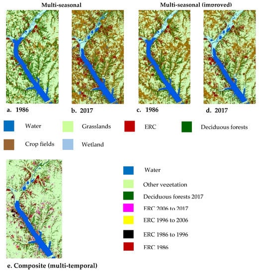
Figure 3.
Image preparation method comparisons. Multi-seasonal SVM classification (a) 1986 and (b) 2017. Multi-seasonal (improved) classification (c) 1986 and (d) 2017. (e) Composite (multi-temporal) image classification with SVM.
As an evergreen tree species, the spectral reflectance of ERC remains relatively constant throughout the year compared to other vegetation in the landscape. Presence of other photosynthetically active vegetation in the surrounding area, such as winter wheat during the dormant season, as well as grasslands, deciduous forests, and crop fields during the growing season, might create confusion with the ERC cover type when a single-date image classification is employed [18]. Therefore, the idea of using a multi-seasonal image stack is to allow the classification algorithm to utilize the relatively constant spectral reflectance of ERC to distinguish it from other vegetation demonstrating a fluctuating reflectance signal.
Post-classification inspection suggested that certain misclassifications can be avoided through improving the training area selection procedure. In this region, it is common to see burnt grasslands and fallowed crop fields that are not in production during the season of interest. Therefore, two additional classes, burnt areas and fallowed crop fields, were trained. However, once the classification was completed, fallowed crop fields and burnt areas were clumped into the agriculture and grassland classes, respectively, to generate the final classification images (Figure 3c,d).
2.3.2. Composite/Multi-Temporal Image Analysis with SVMs
Combining all the images from different time points into a multi-temporal dataset to classify change classes, is known as a type of composite image analysis. This method was successfully used with Landsat satellite images and an SVM classification, to monitor the invasion of an exotic tree species from 1986 to 2006 in Argentina [34]. The advantage of this method is that it requires only one classification image for the entire study period to depict the spatial pattern of change.
The composite image for SA1 was constructed by layer stacking dormant-season Landsat images for four time periods: 1986, 1996, 2006, and 2017. Training areas were selected for seven classes: ERC cover in 1986, changed to ERC during 1986 to 1996, changed to ERC during 1996 to 2006, changed to ERC during 2006 to 2017, deciduous forests in 2017, other vegetation, and water. Gradual expansion of the ERC cover across the landscape is clearly visible with the final classified image (Figure 3e). However, the selection of training areas for change classes is a very time-consuming task, especially when support data such as imagery with higher resolution is not available.
2.4. Accuracy Assessment
The accuracy assessment for the classification was conducted using a common reference dataset, as it would allow comparisons to be made across different classification approaches. The reference dataset was created with 75 points per class (450 in total). A classified image shapefile was converted to a raster along with the reference dataset. The two raster datasets of the reference and classified maps were combined using the spatial analyst tool. The resulting table was used to construct the confusion matrix and compute the user’s accuracy, producer’s accuracy, overall accuracy, and kappa coefficient (Table 2).
Table 2.
Error matrix for multi-seasonal SVM (improved) classification.
2.5. Assessing ERC Expansion between 1986 and 2017
The use of multi-seasonal layer stacks with an SVM classification was concluded to be the most effective approach to classify the 1986 and 2017 images for the three study areas. Each image was classified using the method outlined in Section 2.3.1. Once the 1986 and 2017 images were classified, they were converted to a raster file format for further processing. A class score was assigned to each landcover class of the two classified images. Using the new class score attribute as the value field, the 1986 image was subtracted from 2017 image. The resulting map consisted of 16 change classes. Hence, the map was reclassified to construct the final change map for each study area with six change classes: (i) deciduous to ERC, (ii) non-forest to ERC, (iii) ERC lost, (iv) ERC stable, (v) deciduous stable, and vi) all other. The non-forest to ERC category mainly includes conversion of crop fields and grasslands into ERC-dominated areas.
Accuracy Assessment and Area Estimation
The protocol used for accuracy assessment and area estimation followed the recommended good practices for map accuracy assessment and area estimation in land-change studies [35]. This statistically robust methodology is based on three pillars: (i) a stratified random sampling design for the selection of a subset of pixels from each class of the classified image; (ii) an accurate reference dataset, which could label each unit in the sample with high accuracy; and (iii) analysis of data using confusion matrices, and quantification of errors in classification with estimates of overall accuracy, the user’s accuracy (commission error), and the producer’s accuracy (omission error). The strength of this methodology is that it incorporates the estimated errors in classification in estimating the area of change [35]. The final estimations are reported along with computed uncertainties in terms of confidence intervals.
The total areas of different landcover classes in all three study areas were highly variable. Therefore, a stratified random sampling procedure was followed for the selection of samples from each class. Landsat satellite imagery along with high-resolution NAIP and GoogleEarthTM imagery were used to gather reference information. The complete procedure from sample size determination to final area estimations followed the good practices guidelines [35].
3. Results and Discussion
3.1. Selecting the Most Effective Classification Scheme
The initial comparisons between classification techniques were conducted using single-date Landsat layer-stacks for the study area surrounding the Tuttle Creek reservoir. The two unsupervised techniques, k-means clustering (Figure 2c,d) and ISODATA (Figure 2e,f), demonstrated major discrepancies in its classification solutions, compared to the supervised techniques of MLC (Figure 2g,h) and SVM (Figure 2i,j). Clearly, the unsupervised solutions failed to classify the wetland landcover class, as it was misclassified as other vegetation.
In contrast, the supervised classification permitted selection of a training sample from wetland areas, which ultimately reduced the misclassification error. The overall accuracy of classification for the two unsupervised techniques were less than 0.50, whereas the supervised classification solutions achieved higher accuracies, between 0.84 and 0.91. This improved classification accuracy of the supervised methods over the unsupervised methods are clearly reflected in Figure 4. Hence, supervised classification was preferred over unsupervised classification.
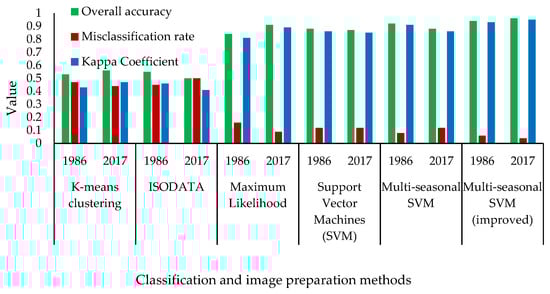
Figure 4.
Comparison of classification accuracies for different classification and image preparation methods.
The solutions derived through the MLC and SVM classifications were comparable to each other (Figure 4). Misclassifications were recorded for deciduous forests with wetlands and agricultural lands, which were common to both MLC and SVM classifications, and more pronounced with the 1986 image. This caused the user’s accuracy for deciduous forests in the 1986 classified image to be drastically reduced, and with the MLC solution, it was around 61%. There was little difference between MLC and SVM classification solutions at this point. However, they have major differences with respect to their functionality. MLC requires normality in the dataset, whereas SVM is a non-parametric statistical learning technique. Within this study, it is not guaranteed that the dataset will follow a normal distribution. Additionally, SVM has the capability of attaining a higher classification accuracy even with a limited training sample [30]. Thus, due to its functional superiority, SVM was chosen as the classification technique best suited for this study.
The selected SVM classification method was employed to classify the two multi-seasonal images for 1986 and 2017, respectively (Figure 3a,b). The corresponding error matrices revealed a slight improvement over single-date image classification (Figure 4). The same multi-seasonal images were classified again after following an improved training area selection process. Result of this improved classification approach (Figure 3c,d) yielded the best accuracy estimates achieved thus far (Figure 4).
Overall accuracies and Kappa coefficients for both 1986 and 2017 image classifications were between 0.93 and 0.96 (Table 2). This approach minimized misclassification errors. User’s accuracy for deciduous forests were 88% and 94% for the 1986 and 2017 images, respectively (Table 2). This is a vast improvement compared to previous solutions. Higher accuracy observed with multi-seasonal imagery in this study is in parallel to the previous findings for this area [18,36].
Finally, a composite image classification was conducted using the SVM technique. The final change map derived through the composite analysis depicted the spatial pattern of ERC expansion over the years (Figure 3e). However, the selection of training areas for change classes is a tedious process. There was much confusion even within a single change class, as one-pixel area represents three decades of change. However, the advantage of this method is the same richness of information in the composite stack of image layers [34]. Identifying pixel trajectories before 2003 was highly complicated due to the unavailability of images with higher resolution, such as NAIP imagery. This was experienced at both the training and accuracy assessment stages. Due to the time-consuming nature of this approach and the complexity of the composite image analysis procedure, the previously characterized multi-seasonal image classification with SVM was concluded as the most effective classification scheme for this study.
Pixel-based image classification of land cover with mixed vegetation is challenging [37]. A crucial task in this study was to distinguish ERC cover from deciduous woodlands and other vegetation. If the study was conducted based only on dormant-season Landsat imagery, a possible complication would be classification of a pixel as ERC, even when it exists underneath a deciduous canopy that is not detected with leaf-off, dormant-season imagery. However, in this study, we used multi-seasonal layer stacks instead of single-date imagery. Multi-seasonal imagery proved to be more effective in classifying land cover in this region with high accuracy. The strength of multi-seasonal imagery is that it incorporates information from the leaf-on, growing season image and from the leaf-off, dormant-season image at the individual pixel level. Therefore, when a pixel is classified into a certain change class, the decision is made based on its spectral reflectance both in the dormant season as well as the growing season. The accuracy assessment was done on the final change map, instead of individually classified maps for a single time point as it does not quantify the accuracy for change classes [38].
3.2. ERC Dynamics within the Three Study Regions
3.2.1. Tuttle Creek Reservoir—SA1
Visual comparison of the two classified images for 1986 and 2017 (Figure 5c,d) clearly illustrates ERC expansion within the study area. The final change map (Figure 5e) further dissects landcover change and ERC expansion based on its trajectory of change. Areas that were originally classified as deciduous forests in 1986 and were classified as converted to ERC in 2017 are depicted in dark blue color. All other land cover classes that went through a similar conversion to become ERC dominated by 2017 are represented in light blue.
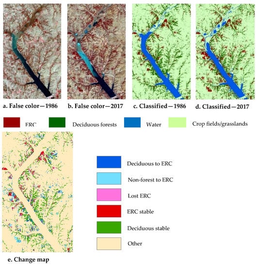
Figure 5.
SA1: Tuttle Creek reservoir. (a) 1986 Landsat TM image, (b) 2017 Landsat OLI image, (c) 1986 classified image, (d) 2017 classified image, and (e) final change map for Study Area 1 (1986 to 2017).
The change map demarcates the areas with lost ERC cover during the study period, as well as stable ERC and deciduous forest stands. All other change and stable classes were clumped together since it is beyond the interests of this study. A relatively smaller portion of the study area is covered by the two classes representing ERC expansion (deciduous to ERC and non-forest to ERC). Grasslands and crop fields dominate this landscape, a situation common throughout the forest–prairie ecotone and is represented by the change class of “other” in this map. Due to this high variability in total area per each change class, the error matrix for the change map is recommended to be reported in terms of area proportions (Table 3) [35]. The estimated area proportions for each change class was used to estimate the area, user’s accuracy, producer’s accuracy, and overall accuracy along with estimations on uncertainty (Table 3).
Table 3.
Area estimation with 95% confidence intervals—Tuttle Creek Reservoir.
The overall accuracy of the change map was estimated to be 0.96 (95% CI: ±0.02). Accuracy estimates for all the classes were above 80%, except for the non-forest to ERC producer’s accuracy. This suggested that a fair amount of ERC expansion into non-forest classes were not documented in the classified image. This is reflected by the non-forest to ERC change class having a 95% confidence interval of around 2000 acres for change area estimation. However, a higher level of precision in classification is observed for other classes. In total, ERC cover has expanded into surrounding areas by about 8200 acres. If lost ERC area is taken into the account, it was estimated that the ERC cover in SA1 has increased by around 6600 acres within the last 30 years (Table 3). The rate of increase is estimated to be a staggering 220 acres per year. Nearly a half of its expansion occurred into the deciduous forests; therefore, it is quite evident that similar to grassland ecosystems [4,9], the deciduous woodlands in this area are affected by the ERC’s rapid expansion.
3.2.2. Perry Reservoir—SA2
Similar to SA1, ERC expansion within this study region was clearly visible with the two classified images (Figure 6c,d). ERC cover was not prominent in the 1986 classified map but exhibited widespread distribution by 2017. This is evident by having a negligible proportion of area for the ERC stable class in the final change map (Table 4). An estimated 99% of the ERC cover mapped in 2017 seemed to have developed after 1986. Representations in the final change map (Figure 6e) were similar to the map constructed for SA1.
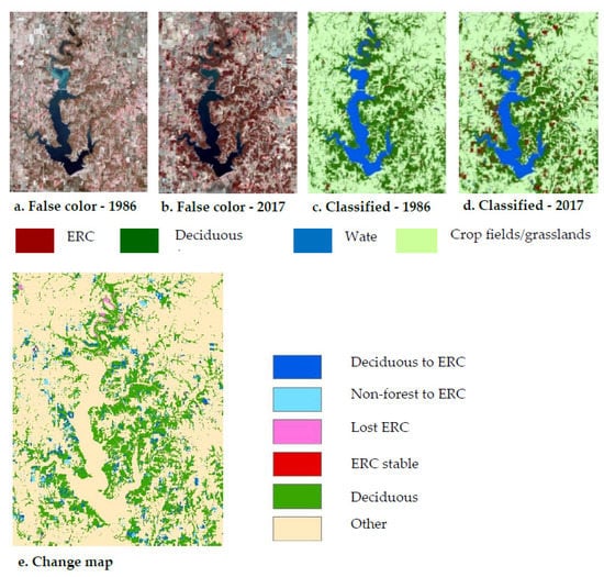
Figure 6.
SA2: Perry reservoir. (a) 1986 Landsat TM image, (b) 2017 Landsat OLI image, (c) 1986 classified image, (d) 2017 classified image, and (e) final change map for study area 2 (1986 to 2017).
Table 4.
Area estimation with 95% confidence intervals—Perry reservoirs.
The estimated overall accuracy of the change map was 0.96 (95% CI: ±0.02). The producer’s accuracy for change classes of non-forest to ERC and ERC lost was around 70% (Table 4). The margin of error was equal or in excess of 50% for these two classes. However, other classes were classified with a higher precision. In this study, our main focus is on the change class of deciduous forests to ERC, which was classified with higher accuracy. The study area has experienced an ERC expansion of 7600 acres within the period of 1986 to 2017, of which a majority (56%) of the expansion occurred into the deciduous forests. The annual rate of ERC expansion within this region was estimated at 216 acres per year, after accounting for lost ERC cover during the same time. Yet again, the astounding rate of ERC expansion within this region is evident with significant impacts on the deciduous forests.
3.2.3. Bourbon County North—SA3
Similar to the other two study regions, ERC expansion is evident with the two classified images for 1986 and 2017 (Figure 7c,d). ERC-dominated areas can be observed in 1986 at the northeast section of the study region (Figure 7c). After 30 years, ERC showed a widespread distribution throughout the study area (Figure 7d). The final change map (Figure 7e) illustrates the spatial trajectories of this ERC expansion, where areas represented in dark blue has undergone a conversion from deciduous forests to ERC by 2017. The pink-colored areas represent ERC expansion into other cover types, including grasslands and abandoned agricultural lands.
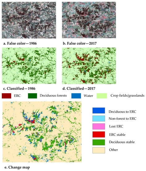
Figure 7.
SA3: Bourbon County North. (a) 1986 Landsat TM image, (b) 2017 Landsat OLI image, (c) 1986 classified image, (d) 2017 classified image, and (e) final change map for Study Area 3 (1986 to 2017).
The overall accuracy of the change map was estimated at 0.95 (±0.03) (Table 5). Compared to the previous two change maps, a higher producer’s accuracy is observed for all the change classes associated with ERC cover (stable, lost, and gained). The margin of error, which is an estimate of the uncertainty as a proportion of the estimated total area, was below 20% for all the classes. The estimated total gain of ERC cover within the 30-year period was about 6500 acres, out of which 71% symbolizes deciduous forest conversions. Once lost ERC cover is taken into the account, the annual rate of expansion of ERC within this region is estimated at 202 acres per year. These observations are comparable with the results obtained for the other two study areas.
Table 5.
Area estimation with 95% confidence intervals—Bourbon County North.
3.3. Impact on Deciduous Woodlands
The final change maps for the three study areas (Figure 5e, Figure 6e, and Figure 7e) spatially illustrates the status changes that occurred with the ERC cover class (stable, lost, and gain). It is evident that ERC has expanded at an alarming rate within all three areas investigated in this study. The rate of expansion exceeded 200 acres per year in all three areas, and the percent increase in ERC cover ranged from around 140% to 540% (Table 6). This astounding rate of expansion of ERC cover was also evident to be having a major impact on the deciduous forests of the region. This is clearly illustrated by Figure 8, which depicts total estimated ERC encroachment for the three study areas, broken down by its impact on deciduous forests and non-forest classes. Conversion of deciduous woodlands to ERC, as a percentage of the total encroachment, were 48%, 56%, and 71%, for SA1, SA2, and SA3, respectively. Eastern redcedar encroachment into the deciduous woodlands as a percentage of existing deciduous woodlands for the three sites were 25%, 13%, and 18%, respectively. This observed ERC encroachment into deciduous woodlands within the forest–prairie ecotone of Kansas, is in parallel to what was reported for other forest types in this region, such as the Cross Timbers of north-central Oklahoma [39] and the glade-like forest types in mid-Missouri [40].
Table 6.
Thirty-year ERC change within the three study areas.
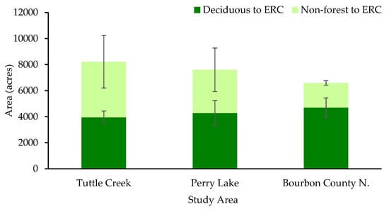
Figure 8.
Total eastern redcedar (ERC) encroachment between 1986 to 2017 in the three study areas, broken down by conversion of deciduous forests and non-forest classes to ERC.
All three study regions are located around recreational areas, such as reservoirs, lakes, and state parks, and includes a large number of rural homeowners. The underlying cause for the observed high ERC expansion could be related to how these lands are managed. ERC is commonly controlled in grasslands using repeated prescribed burns. However, with the presence of dispersed homes in the area, the resulting liability concerns may inhibit the use of periodic burns to control ERC. Thus, it provides conducive environments for ERC to expand into surrounding grasslands, deciduous forests, and abandoned agricultural lands. With continued fire exclusion, ERC gradually expands in area and density. In Kansas, a trend of ERC expansion, in disturbance-free environments, was outlined through FIA inventory data [7]. Further, once ERC starts invading deciduous forests, they have the ability to reduce the fitness of the dominant oak species and facilitate ERC growth, through positive soil–microbe feedbacks and altered litter chemistry [41]. This provides a plausible explanation for the observed ERC expansion into deciduous forests as documented in this study.
In addition to altering species composition and affecting associated ecosystem services, ERC encroachment increases the risk of wildfires [39,42]. Due to its structure, the highly flammable ERC trees can act as ladder fuels, increasing the risk of initiating a crown fire and converting it to a wildfire [18,39]. High flammability of ERC trees was visible during a controlled burn in Kansas [8], where some crowns of standing ERC trees (Figure 9a) and thinned trees lying on the ground (Figure 9b) caught on fire, with flame heights reaching 20 feet or more.
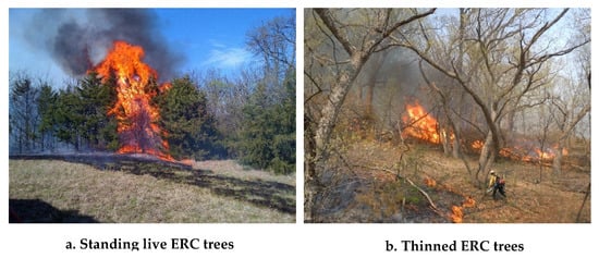
Figure 9.
Highly flammable (a) Live ERC tree crowns and (b) thinned trees lying on the ground caught on fire during a controlled burn in Kansas.
Despite the negative impacts on certain ecosystems, ERC is an essential evergreen element in windbreaks in Kansas [43,44]. Its dense, compact foliage and rapid growth rates make ERC an excellent species to be used in windbreaks to protect crops, shelter livestock, and reduce wind erosion, and also has been found to be providing crop-yield benefits in the Kansas–Nebraska region [45]. Therefore, it is vital to acknowledge its importance in the landscape, while monitoring and managing ERC to prevent its encroachment into surrounding areas [43]. However, accurate information on ERC distribution should be available for land management decisions to be made, especially when rapid expansion is evident. The Kansas Forest Service mapped the statewide rural tree canopy using 2015 NAIP imagery, and this geospatial layer can be used as a baseline for observing tree cover change over time [46].
Prescribed fire is the most effective and economical method of ERC control [43]. Successful control of ERC seedlings with prescribed fires, for oak woodland restoration, has been documented in eastern Kansas [8]. However, it is difficult to kill ERC trees that are taller than 2 m with low-intensity surface fires [47]. Supplementing the burn with thinning ERC trees and saplings would increase the fire intensity and fire effects [48,49,50].
4. Conclusions
This study focused on three study areas that demonstrated high ERC cover in 2017, enabling us to go back in time and characterize the development of the current ERC cover during the past 30-year period. The study reveals that ERC expansion can have a negative impact on the deciduous forests of this region. All three study areas witnessed an ERC expansion in excess of 6000 acres between 1986 and 2017, which accounted for a 139%, 539%, and 283% increase in ERC cover for SA1, SA2, and SA3, respectively. ERC encroachment into deciduous woodlands, as a percentage of the total ERC expansion, was 48%, 56%, and 71% for SA1, SA2, and SA3, respectively. To the best of our knowledge, this is the first multi-year study that investigated ERC expansion effects on deciduous forests using a remote sensing-based methodology in eastern Kansas. Results of this study strongly supports the FIA inventory-based predictions on possible future alterations in species composition in this region [6]. This would negatively impact the oak-dominated woodlands in the region, which are already undergoing a rapid species compositional change due to prolonged fire suppression [1,51]. High ERC expansion would also have adverse effects on the surrounding environment due to the increased wildfire risk.
The lesson learned in this study strongly affirm that the remaining deciduous woodlands of this region should be managed with appropriate silvicultural techniques, such as prescribed burning and mechanical thinning to reduce future ERC dominance. Optimal incorporation of ERC control measures with long-term oak restoration goals is recommended for oak-dominated woodlands of this region where rapid ERC encroachment is documented.
Author Contributions
Conceptualization and methodology, G.A.P.G. and J.W.; formal analysis, investigation, and writing—original draft preparation, G.A.P.G.; validation and writing—review and editing, J.W. and C.J.B.; supervision, and funding acquisition, C.J.B. All authors have read and agreed to the published version of the manuscript.
Funding
Partial funding for this work was provided by the Renewable Resources Extension Act program.
Acknowledgments
Special thanks to Carol Baldwin, Walter Fick, and Will Boyer of Kansas State University, and Ryan Armbrust of Kansas Forest Service for the assistance provided during the site selection and study design phase.
Conflicts of Interest
The authors declare no conflict of interest.
References
- DeSantis, R.D.; Hallgren, S.W.; Stahle, D.W. Drought and fire suppression lead to rapid forest composition change in a forest-prairie ecotone. Forest Ecol. Manag. 2011, 261, 1833–1840. [Google Scholar] [CrossRef]
- Bailey, R.G.; Avers, P.E.; King, T.; McNab, W.H. Ecoregions and Subregions of the United States; 1:7,500,000-Scale Map; USDA Forest Service: Washington, DC, USA, 1994.
- Johnson, P.S.; Shifley, S.R.; Rogers, R. The Ecology and Silviculture of Oak; CABI Publishing: New York, NY, USA, 2009. [Google Scholar]
- Briggs, J.M.; Hoch, G.A.; Johnson, L.C. Assessing the rate, mechanisms, and consequences of the conversion of tallgrass prairie to Juniperus virginiana forest. Ecosystems 2002, 5, 578–586. [Google Scholar] [CrossRef]
- Ratajczak, Z.; Nippert, J.B.; Briggs, J.M.; Blair, J.M. Fire dynamics distinguish grasslands, shrublands and woodlands as alternative attractors in the central great plains of North America. J. Ecol. 2014, 102, 1374–1385. [Google Scholar] [CrossRef]
- Meneguzzo, D.M.; Liknes, G.C. Status and trends of eastern redcedar (Juniperus virginiana) in the central United States: Analyses and observations based on forest inventory and analysis data. J. For. 2015, 113, 325–334. [Google Scholar] [CrossRef]
- Moser, W.K.; Hansen, M.H.; Atchison, R.L.; Butler, B.J.; Crocker, S.J.; Domke, G.; Kurtz, C.M.; Lister, A.; Miles, P.D. Kansas’ forests 2010. In Resource Bulletin; NRS-85; USDA Forest Service, Northern Research Station: Newtown Square, PA, USA, 2013; p. 63. [Google Scholar]
- Galgamuwa, G.A.P.; Barden, C.J.; Hartman, J.; Rhodes, T.; Bloedow, N.; Osõrio, R. Ecological Restoration of an Oak Woodland within the Forest-Prairie Ecotone of Kansas. For. Sci. 2018, 65, 48–58. [Google Scholar] [CrossRef]
- Briggs, J.M.; Knapp, A.K.; Brock, B.L. Expansion of woody plants in tallgrass prairie: A fifteen-year study of fire and fire-grazing interactions. Am. Midl. Nat. 2002, 147, 287–294. [Google Scholar] [CrossRef]
- Ratajczak, Z.; Briggs, J.M.; Goodin, D.G.; Luo, L.; Mohler, R.L.; Nippert, J.B.; Obermeyer, B. Assessing the potential for transitions from tallgrass prairie to woodlands: Are we operating beyond critical fire thresholds? Rangel. Ecol. Manag. 2016, 69, 280–287. [Google Scholar] [CrossRef]
- Leis, S.A.; Blocksome, C.E.; Twidwell, D.; Fuhlendorf, S.D.; Briggs, J.M.; Sanders, L.D. Juniper invasions in grasslands: Research needs and intervention strategies. Rangelands 2017, 39, 64–72. [Google Scholar] [CrossRef]
- Homer, C.G.; Aldridge, C.L.; Meyer, D.K.; Schell, S.J. Multi-scale remote sensing sagebrush characterization with regression trees over Wyoming, USA: Laying a foundation for monitoring. Int. J. Appl. Earth Observat. Geoinfor. 2012, 14, 233–244. [Google Scholar] [CrossRef]
- Lillesand, T.; Kiefer, R.W.; Chipman, J. Remote Sensing and Image Interpretation, 7th ed.; John Wiley & Sons: New York, NY, USA, 2015; p. 720. [Google Scholar]
- Sankey, T.T.; Glenn, N.; Ehinger, S.; Boehm, A.; Hardegree, S. Characterizing western Juniper expansion via a fusion of Landsat 5 thematic mapper and LiDAR data. Rangel. Ecol. Manag. 2010, 63, 514–523. [Google Scholar] [CrossRef]
- Vogelmann, J.E.; Tolk, B.; Zhu, Z. Monitoring forest changes in the southwestern United States using multitemporal Landsat data. Remote Sens. Environ. 2009, 113, 1739–1748. [Google Scholar] [CrossRef]
- Mennis, J.; Guo, D. Spatial data mining and geographic knowledge discovery—An introduction. Comput. Environ. Urban Syst. 2009, 33, 403–408. [Google Scholar] [CrossRef]
- Fayyad, U.M.; Piatetsky-Shapiro, G.; Smyth, P. Knowledge discovery and data mining: Towards a unifying framework. In Proceedings of the Second International Conference on Knowledge Discovery and Data Minining (KDD96); AAAI Press: Portland, OR, USA, 1996; pp. 82–88. [Google Scholar]
- Burchfield, D.R. Mapping Eastern Redcedar (Juniperus virginiana L.) and Quantifying its Biomass in Riley County, Kansas. Master’s Thesis, Kansas State University, Manhattan, KS, USA, 2014. [Google Scholar]
- Vogelmann, J.E.; Xian, G.; Homer, C.; Tolk, B. Monitoring gradual ecosystem change using Landsat time series analyses: Case studies in selected forest and rangeland ecosystems. Remote Sens. Environ. 2012, 122, 92–105. [Google Scholar] [CrossRef]
- Masek, J.G.; Vermote, E.F.; Saleous, N.E.; Wolfe, R.; Hall, F.G.; Huemmrich, K.F.; Gao, F.; Kutler, J.; Lim, T. A Landsat surface reflectance dataset for North America, 1990–2000. IEEE Geosci. Remote Sens. Lett. 2006, 3, 68–72. [Google Scholar] [CrossRef]
- Vermote, E.; Justice, C.; Claverie, M.; Franch, B. Preliminary analysis of the performance of the Landsat 8/OLI land surface reflectance product. Remote Sens. Environ. 2016, 185, 46–56. [Google Scholar] [CrossRef] [PubMed]
- Tso, B.; Mather, P. Classification Methods for Remotely Sensed Data; CRC Press: Boca Raton, FL, USA, 2009. [Google Scholar]
- Canty, M.J. Image Analysis, Classification and Change Detection in Remote Sensing: With Algorithms for ENVI/IDL and Python, 3rd ed.; CRC Press: Boca Raton, FL, USA, 2014. [Google Scholar]
- Rahman, M. Detection of land use/land cover changes and urban sprawl in Al-Khobar, Saudi Arabia: An analysis of multi-temporal remote sensing data. ISPRS Int. J. Geo-Infor. 2016, 5, 15. [Google Scholar] [CrossRef]
- Brannstrom, C.; Jepson, W.; Filippi, A.M.; Redo, D.; Xu, Z.; Ganesh, S. Land change in the Brazilian Savanna (Cerrado), 1986–2002: Comparative analysis and implications for land-use policy. Land Use Pol. 2008, 25, 579–595. [Google Scholar] [CrossRef]
- Memarsadeghi, N.; Mount, D.M.; Netanyahu, N.S.; Le Moigne, J. A fast implementation of the ISODATA clustering algorithm. Int. J. Comput. Geom. Appl. 2007, 17, 71–103. [Google Scholar] [CrossRef]
- Thomson, A. Supervised versus unsupervised methods for classification of coasts and river corridors from airborne remote sensing. Int. J. Remote Sens. 1998, 19, 3423–3431. [Google Scholar] [CrossRef]
- Charaniya, A.P.; Manduchi, R.; Lodha, S.K. Supervised parametric classification of aerial lidar data. In Proceedings of the IEEE 2004 Conference on Computer Vision and Pattern Recognition Workshop (CVPRW’04), Baltimore, MD, USA, 27 June–2 July 2004; Volune 3, pp. 1–8. [Google Scholar]
- Alqurashi, A.F.; Kumar, L. Land use and land cover change detection in the Saudi Arabian desert cities of Makkah and Al-Taif using satellite data. Adv. Remote Sens. 2014, 3, 106–119. [Google Scholar] [CrossRef]
- Mountrakis, G.; Im, J.; Ogole, C. Support vector machines in remote sensing: A review. ISPRS J. Photogr. Remote Sens. 2011, 66, 247–259. [Google Scholar] [CrossRef]
- Taati, A.; Sarmadian, F.; Mousavi, A.; Pour, C.T.H.; Shahir, A.H.E. Land use classification using support vector machine and maximum likelihood algorithms by Landsat 5 TM images. Walailak J. Sci. Technol. (WJST) 2015, 12, 681–687. [Google Scholar]
- Huang, C.; Davis, L.; Townshend, J. An assessment of support vector machines for land cover classification. Int. J. Remote Sens. 2002, 23, 725–749. [Google Scholar] [CrossRef]
- Christianini, N.; Shawe-Taylor, J. An Introduction to Support Vector Machines and Other Kernel-Based Learning Methods; Cambridge University Press: Cambridge, UK, 2000. [Google Scholar]
- Gavier-Pizarro, G.I.; Kuemmerle, T.; Hoyos, L.E.; Stewart, S.I.; Huebner, C.D.; Keuler, N.S.; Radeloff, V.C. Monitoring the invasion of an exotic tree (Ligustrum lucidum) from 1983 to 2006 with Landsat TM/ETM satellite data and support vector machines in Córdoba, Argentina. Remote Sens. Environ. 2012, 122, 134–145. [Google Scholar] [CrossRef]
- Olofsson, P.; Foody, G.M.; Herold, M.; Stehman, S.V.; Woodcock, C.E.; Wulder, M.A. Good practices for estimating area and assessing accuracy of land change. Remote Sens. Environ. 2014, 148, 42–57. [Google Scholar] [CrossRef]
- Hoch, G.A.; Briggs, J.M. Expansion of eastern red cedar (Juniperus virginiana) in the northern Flint Hills, Kansas. In Proceedings of the 16th North American Prairie Conference; Springer, J.T., Ed.; University of Nebraska: Kearney, Nebraska, USA, 1999; pp. 9–15. [Google Scholar]
- Wang, J.; Xiao, X.; Qin, Y.; Dong, J.; Geissler, G.; Zhang, G.; Cejda, N.; Alikhani, B.; Doughty, R.B. Mapping the dynamics of eastern redcedar encroachment into grasslands during 1984–2010 through PALSAR and time series Landsat images. Remote Sens. Environ. 2017, 190, 233–246. [Google Scholar] [CrossRef]
- FAO. Map Accuracy Assessment and Area Estimation: A Practical Guide; National Forest Monitoring Assessment Working Paper No. 46/E; Food and Agriculture Organization of the United Nations: Rome, Italy, 2016; Available online: http://www.fao.org/3/a-i5601e.pdf (accessed on 18 October 2017).
- Hoff, D.; Will, R.; Zou, C.; Lillie, N. Encroachment dynamics of Juniperus virginiana L. and mesic hardwood species into cross timbers forests of North-Central Oklahoma, USA. Forests 2018, 9, 75. [Google Scholar] [CrossRef]
- Knapp, B.O.; Pallardy, S.G. Forty-Eight Years of Forest Succession: Tree Species Change across Four Forest Types in Mid-Missouri. Forests 2018, 10, 633. [Google Scholar] [CrossRef]
- Williams, R.J.; Hallgren, S.W.; Wilson, G.W.; Palmer, M.W. Juniperus virginiana encroachment into upland oak forests alters arbuscular mycorrhizal abundance and litter chemistry. Appl. Soil Ecol. 2013, 65, 23–30.
- Twidwell, D.; Fuhlendorf, S.D.; Taylor, C.A., Jr.; Rogers, W.E. Refining thresholds in coupled fire–vegetation models to improve management of encroaching woody plants in grasslands. J. Appl. Ecol. 2013, 50, 603–613. [Google Scholar] [CrossRef]
- Armbrust, R.; Carlson, D.; Hartman, J.; McDonnell, T.; Paul, D.; Williams, J.; Yoder, A.; Biles, L. Eastern Redcedar Expansion: Perspective, response, and strategy. Agricultural Experiment Station and Cooperative Extension Service, Kansas State University, Manhattan, KS, USA. 2018. Available online: https://www.kansasforests.org/resources/resources_docs/Eastern-Redcedar.pdf (accessed on 13 September 2019).
- Strine, J.H. Windbreaks for Kansas. Agricultural Experiment Station and Cooperative Extension Service, Kansas State University. MF-2120. 2004. Available online: https://www.bookstore.ksre.ksu.edu/pubs/MF2120.pdf (accessed on 13 September 2019).
- Osorio, R.J.; Barden, C.J.; Ciampitti, I.A. GIS approach to estimate windbreak crop yield effects in Kansas–Nebraska. Agrofor. Syst. 2019, 93, 1567–1576. [Google Scholar] [CrossRef]
- Paul, D.A.; Whitson, J.W.; Marcotte, A.L.; Liknes, G.C.; Meneguzzo, D.M.; Kellerman, T.A. High-resolution land cover of Kansas (2015); Updated 27 November 2017; Forest Service Research Data Archive: Fort Collins, CO, USA; Available online: https://doi.org/10.2737/RDS-2017-0025 (accessed on 29 October 2019).
- Ansley, R.J.; Wiedemann, H.T. Reversing the woodland steady state: Vegetation responses during restoration of Juniperus-dominated grasslands with chaining and fire. Western North American Juniperus Communities; Springer: New York, NY, USA, 2008; pp. 272–290. [Google Scholar]
- Weir, J.R.; Derek, S.J. Ignition and fire behaviour of Juniperus virginiana in response to live fuel moisture and fire temperature in the southern Great Plains. Int. J. Wildl. Fire 2014, 23, 839–844. [Google Scholar] [CrossRef]
- Galgamuwa, G.A.P. Ecological Restoration of an Oak Woodland in Kansas Informed with Remote Sensing of Vegetation Dynamics. Ph.D. Dissertation, Kansas State University, Manhattan, KS, USA, 2017. [Google Scholar]
- Simões, L.H.P. Effects of Prescribed Burning and Thinning on Oak Regeneration in Northeast Kansas. Master’s Thesis, Kansas State University, Manhattan, KS, USA, 2019. [Google Scholar]
- Nowacki, G.J.; Abrams, M.D. The demise of fire and “mesophication” of forests in the eastern United States. BioScience 2008, 58, 123–138. [Google Scholar] [CrossRef]
© 2020 by the authors. Licensee MDPI, Basel, Switzerland. This article is an open access article distributed under the terms and conditions of the Creative Commons Attribution (CC BY) license (http://creativecommons.org/licenses/by/4.0/).