A Wavelet-Based Evolving Fuzzy Framework for Fault Diagnosis in the Tennessee Eastman Process

Abstract

Evolving fuzzy systems (EFS) offer an incremental learning, making them promising for fault diagnosis (FD) in industrial processes, where unknown faults and changing operation conditions are common. The evolving fuzzy structure enables incremental rule adaptation while maintaining interpretability and reduced computational complexity compared with deep learning approaches. However, the performance of EFS depends heavily on the preprocessing of input data. This study evaluates eight preprocessing strategies for EFS applied to the Tennessee Eastman benchmark process. A one-vs-rest EFS architecture was implemented for ten representative faults (IDV1, IDV2, IDV4, IDV5, IDV6, IDV7, IDV8, IDV10, IDV13 and IDV14) in order to make a comparison with other FD techniques. This approach uses seven variables selected by using the least angle regression. Preprocessing methods were applied to highlight fault signatures. Using the Daubechies-4 in the preprocessing achieved the best overall F1-score (73.68%) with a sensitivity of 97.37%, outperforming the no-preprocessing baseline (F1 = 70.67%). Per-fault analysis showed high performance for faults IDV6, IDV7, and IDV14, while IDV1, IDV2, IDV5, and IDV8 exhibited high sensitivity but lower specificity. These findings indicate that wavelet preprocessing significantly enhances EFS for FD, and that the choice of wavelet should be guided by application priorities: Daubechies-4 is recommended for maximum detection and fewer false alarms. The obtained results demonstrate that wavelet preprocessing substantially improves classification robustness and fault discrimination compared with the non-preprocessed baseline.

1. Introduction

In modern industrial processes, fault diagnosis (FD) is essential to detect anomalies that can lead to equipment degradation, safety risks, environmental harm, expensive corrective maintenance, and expensive unplanned shutdowns [1,2]. The growing complexity of industrial systems, tighter profit margins, stricter product specifications, and more stringent safety regulations have fueled the need for advanced, reliable, and interpretable fault diagnosis solutions [3].

The Tennessee Eastman (TE) process continues to be a standard benchmark for evaluating FD algorithms [4]. The TE process, which was first proposed by Downs and Vogel in 1993 [5], simulates a realistic chemical plant with 20 predefined faults, 41 measured variables, 12 manipulated variables, and five major unit operations. Its widespread use has enabled comparisons of various FD approaches, ranging from statistical methods (PCA, PLS, ICA) [6] to machine learning methods (support vector machines, neural networks) [7,8] and fuzzy systems [9,10].

Conventional FD techniques often operate in offline batch mode, where a model is trained once using historical data and then deployed for monitoring [11]. While effective in stationary settings, batch-trained models suffer from several drawbacks in practical industrial environments:

• Incapacity to handle unknown faults: The model typically fails to identify a fault not presented in the training data, often misclassifying it as normal operation [12].
• Lack of flexibility: Changes in process dynamics, raw material characteristics, environmental factors, set-points, or equipment wear can render the original model obsolete over time [13].
• Computational limitations: Retraining from scratch on growing historical datasets becomes increasing costly in terms of memory and time [14].

Evolving fuzzy systems (EFS) have emerged as an interesting approach for adaptive learning from data streams in order to overcome these constraints [15,16]. Unlike traditional fuzzy systems built in batch mode, EFS offer:

• Incremental learning: Samples are processed one at a time (or in blocks) without storing the entire dataset, making EFS suitable for streaming data and big data scenarios [17]; no epochs for training are needed.
• Structural evolution: New rules can be added when new operating conditions or system states emerge, and outdated or redundant rules can be eliminated to preserve compactness and interpretability [18].
• Rapid adaptation: Recursive updating of consequent parameters (e.g., linear functions in Takagi–Sugeno systems) enables fast adaptation to process changes [19].

Several EFS architectures have been proposed in the literature, including eTS [20], FLEXFIS [21], SAFIS [22], PANFIS [23], and GENEFIS [24]. Extensive surveys are available in [25,26]. Significantly, EFS has been effectively applied to fault diagnosis in various industries, such as rolling mills [27], chemical processes like the Tennessee Eastman process [28], and NO_x emission monitoring [29].

Incipient faults, those that initially cause minor deviations from normal behavior and are often masked by measurement noise, control actions, and typical process variability, are difficult to detect until they produce noticeable process changes. These faults represent a recurring challenge in FD [30]. Wavelet transforms offer multi-resolution analysis capable of simultaneously capturing high-frequency transients and low-frequency trends, making them highly successful for FD [31].

Wavelet-based techniques have produced impressive results on the TE process. For example, D’Angelo et al. [32] achieved an average sensitivity of 88.52% by combining fuzzy clustering with wavelets and beta distributions. Hajihosseini et al. [33] achieved a sensitivity of 98.6% for specific faults by using discrete wavelet transform (DWT) to extract bi-dimensional features fed into a neural network classifier. Wavelet-based deep learning architectures have been proposed for TE fault diagnosis [34,35].

In [36], Daubechies-4 and Polywoq4 wavelets were used to preprocess TE signals prior to classification using an inverse fuzzy model. Although DWT with eight decomposition levels proved particularly effective for highlighting fault signatures, it required 256 samples (approximately 12.8 h) before fault isolation can be performed. This delay motivated the investigation of alternative preprocessing techniques and an examination of detection speed, sensitivity, and specificity.

Despite the individual successes of wavelet preprocessing and EFS, several research gaps remain:

• Limited integration: Few studies have systematically integrated EFS with wavelet preprocessing for adaptive FD, despite the complementary advantages of both methods.
• Absence of comparative studies: No thorough comparison exists within the EFS framework of various preprocessing techniques (smoothing, differentiation, peak detection, and standard wavelets).
• Open-source implementations: Most EFS implementations are proprietary or only accessible in commercial environments like MATLAB© 2015b, hindering reproducibility and adoption in academic and industrial settings.

This article fills these gaps with the following contributions:

• Integration of EFS with wavelet preprocessing: A complete, modular implementation of EFS with one-vs-rest architecture for multi-fault classification in the TE process.
• Comparative study: Evaluation of eight preprocessing methods, including none, smoothing, peak detection, balanced preprocessing, strong smoothing, and the Daubechies, Haar, and Coiflet wavelets (all at level 4).
• Open-source implementation: The entire codebase is implemented in Octave©, a free and open-source MATLAB© alternative, ensuring full reproducibility.
• Detailed per-fault analysis: Results are reported not only as averages but also per individual fault (IDV1, IDV2, IDV4, IDV5, IDV6, IDV7, IDV8, IDV10, IDV13 and IDV14), revealing which faults are most challenging for EFS.

Unlike conventional FD approaches based exclusively on static classifiers or deep learning architectures requiring extensive retraining, the proposed methodology integrates evolving fuzzy systems with wavelet-based preprocessing in an adaptive framework oriented to industrial fault diagnosis. The contribution of this work is not centered on the development of a new standalone classifier, but rather on combining online rule evolution, incremental structural adaptation, and multi-resolution signal preprocessing for handling nonlinear process dynamics under changing operating conditions.

Furthermore, the proposed framework evaluates the influence of different wavelet families on the performance of evolving fuzzy diagnosis systems on the Tennessee Eastman benchmark. The results demonstrate that the preprocessing stage strongly affects the sensitivity, specificity, and robustness of the evolving classifier. Therefore, this work provides practical insights regarding the integration of signal processing and adaptive fuzzy inference for fault diagnosis in complex industrial systems.

The experimental results, summarized in Table 1, demonstrate that:

Table 1. Selected faults in the TE process.

Fault ID	Description	Type	Difficulty
IDV1	A/C feed ratio change	Step	Easy
IDV2	B composition change	Step	Easy
IDV4	Cooler water temperature change	Step	Easy
IDV5	Condenser temperature change	Step	Easy
IDV6	A feed loss	Step	Medium
IDV7	Separator pressure change	Step	Medium
IDV8	Reactant composition change	Random	Medium
IDV10	C feed temperature	Random	Hard
IDV13	Slow drift in reaction kinetics	Drift	Hard
IDV14	Sticking valve	Structural	Hard

• The Daubechies wavelet approach greatly outperforms the baseline without preprocessing (F1 = 70.67%), achieving the best overall F1-score (75.50%) with sensitivity of 97.17%.
• When false alarms are expensive, the Haar wavelet is preferred because it has the highest specificity (44.37%).
• The Coiflet wavelet performs poorly (F1 = 65.15%), especially on fault IDV7 (sensitivity = 17.33%), indicating that this application is not a good fit for it.
• While some faults (IDV1, IDV2, IDV5, IDV8 and IDV13) are still difficult to diagnose, frequently showing 100% of sensitivity but the specificity is around 50%, others (IDV6, IDV7, and IDV14) are diagnosed with extremely high accuracy (F1 > 94% with the best method).

These results emphasize how crucial it is to adjust preprocessing techniques to particular fault kinds and application needs (sensitivity vs. specificity trade-offs).

The remainder of the paper is structured as follows. Section 2 describes the Tennessee Eastman process, the selected faults and dataset, the principles of evolving fuzzy systems, the one-versus-rest architecture, the evaluated wavelet preprocessing techniques, and the experimental setup. Section 3 reports and discusses the results, including per-fault analysis and method comparisons. Section 4 presents the conclusions and contributions. Finally, Section 5 discusses limitations and future directions.

2. Materials and Methods

This section describes the materials and methods used in this investigation. First, the Tennessee Eastman (TE) benchmark process is introduced, including its key components, the ten faults selected for comparison with similar techniques, and the characteristics of the dataset used. Second, the principles of evolving fuzzy systems (EFS) are presented, including the recursive parameter adaptation mechanism, the Takagi–Sugeno rule structure, the one-vs-rest architecture for multi-fault classification, and the rule evolution and pruning criteria. Third, the wavelet-based preprocessing techniques evaluated in this study are described, including the Haar, Coiflet, and Daubechies wavelets, along with several traditional preprocessing methods that served as baselines. Finally, the experimental setup, including data partitioning, hyperparameter selection, evaluation metrics, and implementation details in the GNU Octave© 5.1.0 environment, is described in detail.

2.1. Tennessee Eastman Process Description

The Tennessee Eastman (TE) process is a widely recognized benchmark for fault diagnosis (FD) studies [5]. Originally it was developed by Downs and Vogel; it simulates a realistic chemical plant with five major unit operations: a reactor, a product condenser, a recycle compressor, a vapor–liquid separator, and a product stripper [5]. The process produces two liquid products (G and H) from four gaseous reactants (A, C, D, and E), with an inert component B present in the feed streams. The overall reaction scheme is as follows:

$$A\left(g\right)+C\left(g\right)+D\left(g\right)\to G\left(\mathit{liq}\right),$$

(1)

$$A\left(g\right)+C\left(g\right)+E\left(g\right)\to H(\mathit{liq}),$$

(2)

$$A\left(g\right)+E\left(g\right)\to F(\mathit{liq}),$$

(3)

$$3D\left(g\right)\to 2F(\mathit{liq}),$$

(4)

The TE process model includes 41 measured variables (x₁ to x₄₁) and 12 manipulated variables. The first 22 measurements are sampled every 3 min, while the remaining 19 composition variables have longer delay times (6–15 min) due to analysis requirements [4]. A total of 20 predefined faults (IDV1 to IDV20) are available for simulation, covering different fault types including step changes, random variations, slow drifts, and valve sticking [5].

In this work, ten representative faults were selected based on their prevalence in the literature, to compare results, and because of their varying difficulty levels [6,7,32]. Table 1 summarizes the selected faults and their characteristics.

The TE process simulations under both normal operating conditions and each of the ten chosen faults provided are used. Three severity levels are available for each fault. In accordance with standard procedure, the medium severity level was chosen to balance practical relevance and detection difficulty [36]. Each simulation run contains 2001 samples. Faults are introduced at sample 501 and removed at sample 1011 (500 normal samples, 511 fault samples, and 990 post-fault samples). The sampling time in the TE process is three minutes. The data used were obtained from simulations because original data available for non-Simulink© users contain fault data, and the post-fault behavior is also relevant for FD.

Seven measured variables were chosen as inputs for the EFS classifier in accordance with the variable selection methodology described in [15]; the variables are x₁, x₄, x₁₈, x₂₁, x₂₃, x₂₅, and x₂₈. Least angle regression (LARS) was used to determine which variables were most informative for fault isolation. After normalizing the data to zero mean and unit standard deviation using parameters estimated from normal operating data, clipping was used to restrict extreme values to the range [−3, 3].

LARS builds a model incrementally by adding the predictor most correlated with the current residual. Also, LARS moves in a direction equiangular between the selected predictors, ensuring monotonic progression of the L₁ norm of the coefficient vector while maintaining the same computational cost as ordinary least squares. The algorithm proceeds as follows:

• Computation of the correlations between each predictor and the current residual: $\mathrm{c}={\mathrm{X}}^{\mathrm{T}}\left(\mathrm{y}-\mathrm{X}\mathsf{\beta }\right)$.
• To identify the most correlated predictor: $\widehat{\mathrm{c}}={\max }_{\mathrm{j}}\left|{\mathrm{c}}_{\mathrm{j}}\right|$.
• To move the coefficient vector in the least angle direction until another predictor attains the same correlation.
• To add the new predictor to the active set and return to step 1.

For the TE process, LARS was applied to the full set of 41 measured variables. The seven variables with the largest absolute regression coefficients were from the solution of

$${min}_{\beta } {‖y-X\beta ‖}_2^2+\alpha {‖\beta ‖}_1,$$

(5)

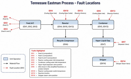
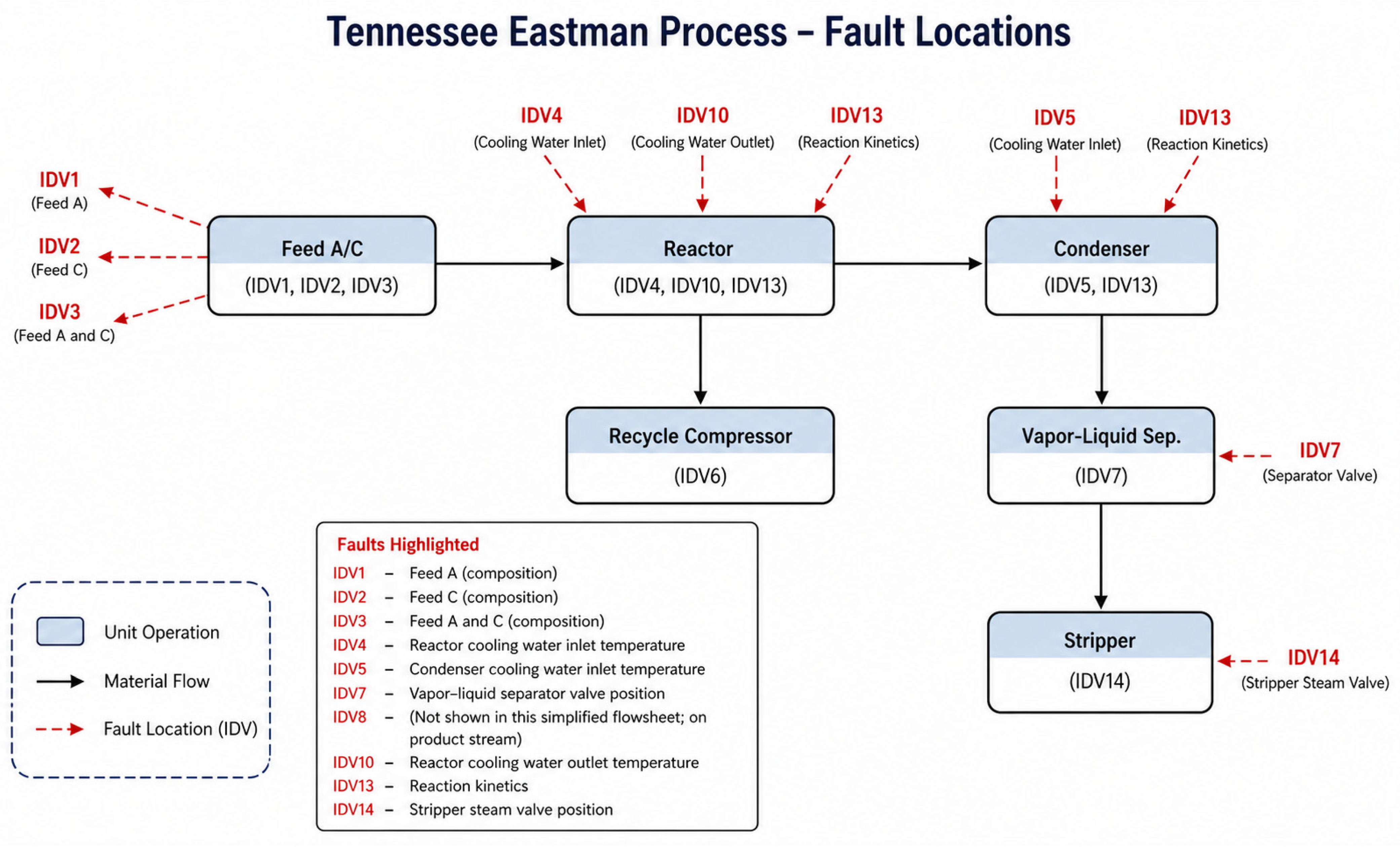
with X being the normalized data matrix with zero mean, y the target output vector, and β the coefficient to find. α is a regularization parameter that controls the sparsity of the solution. A scheme of fault locations in the TE process is shown in Figure 1, illustrating the components of the industrial process.

Figure 1. Fault locations in the TE process.

2.2. Evolving Fuzzy Systems

A class of adaptive fuzzy inference systems known as evolving fuzzy systems (EFS) gains incremental, single-pass knowledge from data streams [15]. In contrast to traditional fuzzy systems that are trained in batch mode, EFS offers three essential features:

• Incremental learning: They allow incremental operation and handling of unbounded data streams by processing data samples one at a time (or in blocks) without storing the complete dataset [17]. In this work, the data were split to evaluate our approach: 85% of the data were used to evolve the fuzzy system after certain preprocessing, and the remaining 15% were used to evaluate the methodology.
• Structural evolution: When the existing system cannot adequately represent new data patterns, the rule base can grow by adding new rules or shrink by removing unnecessary or redundant rules [18].
• Parameter adaptation: Forgetting mechanisms are used to recursively update both antecedent (membership function parameters) and consequent parameters to monitor evolving process dynamics [19].

A Takagi–Sugeno (TS) fuzzy model was used with local learning in this work, in which every rule has a linear consequent function. For regression tasks, the fuzzy rule has the following form:

$$\begin{gathered} {\mathrm{Rule}}^i:\mathrm{If} \left(x_1 \mathrm{is} {\mu }_{i1}\right) \mathrm{and}\dots \mathrm{and} {(x}_p \mathrm{is} {\mu }_{ip}), \mathrm{then} y=w_{i0}+w_{i1}{x}_1+ \\ \dots +w_{ip}{x}_p, \end{gathered}$$

(6)

where ${\mu }_i$ is a fuzzy set, x is the input data, and $w_i$ are the weights of the consequent. The consequent reduces to a singleton value that represents the estimated probability of the fault class for binary classification (fault vs. normal), which is then thresholded to yield a clear decision.

A one-vs-rest classification architecture was used to manage various fault types [26]. Separate binary EFS classifiers are trained for each of the ten selected faults. During operation, all classifiers are evaluated concurrently, and the classifier with the highest activation, or the first to surpass a confidence threshold, determines the detected fault. This strategy offers several benefits:

• Each binary classifier can be independently optimized for its specific fault.
• New fault types can be added by training additional binary classifiers without retraining existing ones.
• Training each fault against all normal and other fault samples naturally addresses class imbalance.

New rule generation is controlled by a vigilance criterion based on the Mahalanobis distance between the current data sample and existing rule centers [21]. If the minimum Mahalanobis distance is greater than a predetermined threshold (vigilance), which indicates that the sample is in an uncovered area of the input space, a new rule is generated. The current sample is used to initialize the new rule’s center, and a diagonal matrix scaled by ${\sigma }_{\mathrm{i}\mathrm{n}\mathrm{i}\mathrm{t}}^2$ is used to initialize its covariance matrix.

Periodically, a pruning mechanism preserves interpretability and compactness. Rules are assessed based on their age (time since last update) and accuracy (ratio of correct predictions to total samples assigned to the rule). Rules that are too old without updates or have low accuracy (less than 50%) are eliminated. To reduce redundancy, rules with very similar centers (Euclidean distance below a threshold) are merged.

2.2.1. Rule Evolution and Pruning

A new rule is created when the current sample x lies outside the coverage region of all existing rules. In this case, a new data behavior can be detected and represented by the new fuzzy rule. As mentioned above, the Mahalanobis distance is used to determine the coverage area between the sample and the rule center c. The Mahalanobis distance for a rule i is computed as follows:

$$d_M\left(i,x\right)=\sqrt{{{\left(x-c_i\right)}^T\Sigma }_i^{-1}\left(x-c_i\right)},$$

(7)

where ${\Sigma }_i$ is the covariance matrix. The sample is considered to be covered by rule i if $d_M(i,x)\le \rho$, $\rho$ being the vigilance threshold, and if for all existing rules ${\min }_i d_M\left(i,x\right)>\rho$, then a new rule is added with center $c_{new}=x$, the inverse covariance matrix will be ${\Sigma }_i^{-1}=\raisebox{1ex}{$1$}\!\left/ \!\raisebox{-1ex}{${\sigma }_{init}^2$}\right.\mathrm{I}$, and the consequent rule will be ${\theta }_{new}=y_{true}$.

To maintain compactness and to prevent unbounded rule base growth, the pruning procedure is executed every $T_{prune}$ = 50 samples. Algorithm 1 shows the pruning of rules when necessary. A rule is considered redundant and removed if it satisfies any of the following criteria:

• Low accuracy: The rule classification accuracy falls below 50%. The accuracy of rule i computed as

  $${\mathrm{acc}}_{\mathrm{i}}={\displaystyle \frac{\mathrm{correct} \mathrm{predictions}}{\mathrm{total} \mathrm{samples} \mathrm{assigned} \mathrm{to} \mathrm{the} \mathrm{rule}}},$$

  (8)

  and the rule is pruned if ${\mathrm{acc}}_{\mathrm{i}}<0.5$.
• Obsolescence: The rule has not been updated for a large number of samples, i.e., ${\mathrm{age}}_{\mathrm{i}}>{\mathrm{age}}_{\mathrm{m}\mathrm{a}\mathrm{x}}$, where ${\mathrm{age}}_{\mathrm{m}\mathrm{a}\mathrm{x}}=500$ samples in this case.
• Redundancy due to similarity: Two rules are considered too similar (their centers are close) and their consequents are nearly identical. Then rules i and j are merged if

$${‖c_i-c_j‖}_2<{\theta }_{merge}, \mathrm{and} \left|{\theta }_i-{\theta }_j\right|<{\theta }_{\theta },$$

(9)

with ${\theta }_{merge}=0.15$ being the distance threshold, and the consequent similarity threshold being ${\theta }_{\theta }=0.1$. When rules are merged, the one with higher accuracy is retained, and its center is updated as the weighted average of both centers using the number of samples assigned to each rule.

2.2.2. Parameter Adaptation

When a new sample x falls within the coverage region of existing rules, the center of the winning rule (the rule with the smallest $d_M$) is updated using a learning rate η according to

$$c_{win}\left(t\right)=c_{win}\left(t-1\right)+\eta \left(x-c_{win}\left(t-1\right)\right).$$

(10)

The inverse covariance matrix ${\Sigma }_{win}^{-1}$ is adaptively updated using a weighted recursive formulation to capture the local data distribution:

$${\Sigma }_{win}^{-1}\left(t\right)=\left(1-\lambda \right){\Sigma }_{win}^{-1}\left(t-1\right)+\lambda Q\left(t\right),$$

(11)

where

$$Q\left(t\right)={\displaystyle \frac{\left(x-c_{win}\right){\left(x-c_{win}\right)}^T}{{‖x-c_{win}‖}^2+ϵ}},$$

$\lambda =\raisebox{1ex}{$1$}\!\left/ \!\raisebox{-1ex}{$n_{win}+1$}\right.$ is a forgetting factor, and $n_{win}$ is the number of samples assigned to the winning rule. This recursive approximation allows the evolving fuzzy rule to adapt its local covariance structure online while avoiding matrix inversion at every iteration.

Algorithm 1: Pseudocode for the periodic rule pruning

1: Input: Current rule base R, pruning interval T_prune

2: Output: Updated rule base R

3: if (samplecounter mod Tprune = 0), then

4:  for each rule i in R do

5:    Compute acci = correcti/totali

6:    if acci < 0.5, then

7:     Remove rule i

8:    else if agei > agemax, then

9:     Remove rule i

10:   end if

11:  end for

12:  for each pair of rules (i, j) in R do

13:   if (distance(i, j) < θmerge) and (|θi − θj| < θθ), then

14:     Remove rule with lower acci

15:   end if

16:  end for

17: end if

The consequent parameters ${\theta }_i$ for each rule are updated using recursive fuzzily weighted least squares (RFWLS) [21], which performs local learning by weighting each sample’s contribution based on the corresponding rule’s normalized activation. The recursive update equation is

$${\theta }_i\left(t\right)={\theta }_i\left(t-1\right)+K_i\left(t\right)\left(y\left(t\right)-{\phi }_i^T\left(t\right){\theta }_i\left(t-1\right)\right),$$

(12)

where K_i is the Kalman gain matrix calculated from the fuzzily weighted covariance matrix P_i, ${\phi }_i\left(t\right)=\exp \left(-0.5d_M^2(i,x)\right)$ is the regressor vector, and θ_i is the parameter vector for rule i, ($w_{i1}, w_{i2},\dots , w_{ip}$). This local approach ensures that each rule’s consequent is updated only based on samples that activate that rule, weighted by their activation degree.

The normalized activation of rule i is

$${\phi }_{norm}\left(i,t\right)={\displaystyle \frac{{\phi }_i\left(t\right)}{{\sum }_{j=1}^C{\phi }_j\left(t\right)}}.$$

(13)

A modified version of eVQ (evolving Vector Quantization) [21] is used to update antecedent parameters (centers and covariance matrices).

The final decision is obtained from the aggregated output of the EFS. Each fuzzy rule produces a local consequent value based on the activation level of its premise, and these local outputs are combined using a weighted average aggregation mechanism. The resulting aggregated output represents the classifier’s confidence regarding the presence of a specific fault under the one-vs-rest scheme.

For FD, the aggregated output is compared against a fixed decision threshold. In this work, a threshold of 0.5 was employed, such that outputs greater than or equal to 0.5 are classified as fault conditions, while lower values were associated with normal operation. This threshold was selected because it provided stable behavior across the evaluated faults and maintained a suitable balance between sensitivity and specificity during the experimental analysis.

This adaptive behavior is particularly useful in industrial FD because process dynamics may evolve over time due to operating condition changes, sensor degradation, or previously unseen disturbances.

2.3. Wavelet-Based Preprocessing Methods

Because fault signatures are initially subtle and easily obscured by noise and control actions, wavelet transforms offer a multi-resolution analysis capability that is especially helpful for identifying incipient faults [30,31]. In this work, we compare several traditional techniques with three wavelet-based preprocessing methods.

In the proposed methodology, each process variable is preprocessed independently using discrete wavelet decomposition before entering the evolving fuzzy classifier. The original signals were decomposed using Haar, Daubechies, and Coiflet mother wavelets. After decomposition, the approximation coefficients are retained as filtered representations of the process dynamics, while high-frequency components associated mainly with noise were attenuated. These reconstructed signals are subsequently normalized and used as inputs for the EFS. This preprocessing stage aims to improve fault-related feature representation while preserving the temporal behavior of the original process variables.

The preprocessing stage was based on discrete wavelet transform (DWT), where each process signal x(nT) was decomposed into approximation and detail coefficients through successive low-pass and high-pass filtering operations:

$$x\left(nT\right)\to \left\{A_j\left(nT\right), D_j\left(nT\right)\right\},$$

(14)

where A_j(nT) represents the approximation coefficients, D_j(nT) are the detail coefficients at decomposition level j, and T is the sample time of three minutes. These reconstructed signals were subsequently normalized and used as inputs to the EFS.

2.3.1. Daubechies-4 (db4) Wavelet

The db4 wavelet transform uses differences in moving averages at several scales to approximate the effect of discrete wavelet decomposition. The detail coefficient at scale k for a given signal x(t) is calculated as follows:

$$d_k\left(t\right)=\left|{\mathrm{MA}}_{2k}\left(x\left(t\right)\right)-{\mathrm{MA}}_{2k+1}\left(x\left(t\right)\right)\right|,$$

(15)

where a moving average with window size w is indicated by MA_w. The total detail coefficients for all scales, normalized to [0, 1], constitute the final preprocessed signal. This approach can be used in typical scientific computing environments instead of classical db4 wavelet because it captures multiscale transitions without the need for a specialized wavelet toolbox.

2.3.2. Haar Wavelet

The Haar wavelet, which has a square-shaped scaling function, is the most basic orthogonal wavelet [37]. It works well for identifying sudden changes (step-type faults) and is computationally efficient. The discrete Haar wavelet transform decomposes the signal into approximation and detail coefficients at several levels. In this work, we use level-4 decomposition and reconstruct the signal using only the detail coefficients, which emphasize fault onsets and transients.

2.3.3. Coiflet Wavelet

Coiflet wavelets, especially coif4, are more symmetric than Daubechies wavelets and offer superior reconstruction capabilities. They are frequently chosen when the phase of signal components needs to be preserved. As with the Haar wavelet, we use level-4 decomposition and retain the detail coefficients for fault highlighting.

2.3.4. Conventional Preprocessing Techniques

For comparison, we also evaluate five conventional preprocessing methods:

• None: Normalized raw data (baseline).
• Smoothing: Moving average with window size 3.
• Peak detection: Deviations greater than two standard deviations determine the binary threshold.
• Adaptive thresholding comes after normalization in balanced preprocessing.
• Moving average with window size 7 is a strong smoothing technique.

2.4. Experimental Setup

A training set (85%, first 1700 samples) was used to evolve the fuzzy system, not for training, allowing the fuzzy system to be adapted according to incoming data. The validation set (15%, remaining 301 samples) was created from the available data (2001 samples) for each fault to evaluate the proposed framework according to its evolving property. The partitioning of normal operating data was comparable. To address class imbalance, we used undersampling of normal samples with a ratio of two normal samples for every fault sample during training.

The hyperparameters shown in Table 2 were selected empirically based on preliminary experiments and stability analysis over several TE fault scenarios. Parameters related to rule evolution, such as vigilance threshold and pruning frequency, were adjusted to balance model adaptability and rule base compactness. Learning rate parameters were selected to ensure stable incremental adaptation without excessive oscillations. The same hyperparameter configuration was maintained for all experiments to ensure consistency and reproducibility.

Table 2. ESF hyperparameters (default values).

Parameter	Symbol	Default Value	Description
Vigilance	Ρ	1.2	Threshold for creating new rules
Learning rate	H	0.05	Step size for center/consequent updates
Initial spread	σinit	0.5	Initial width of Gaussian membership functions
Maximum rules	Rmax	40	Upper bound on rule base size
Minimum samples per rule	Nmin	20	Samples required before pruning
Pruning interval	Tprune	50	Frequency of pruning (samples)
Persistence	Npersist	2	Consecutive detections required
Detection threshold	λ	0.25	Decision threshold for binary classification
Max age before pruning	${\mathrm{age}}_{\mathrm{m}\mathrm{a}\mathrm{x}}$	500	Samples without update
Merge distance threshold	${\theta }_{merge}$	0.15	Max center distance for merging
Merge consequent threshold	${\theta }_{\theta }$	0.1	Max consequent difference for merging
Persistence window	$N_{persist}$	2	Consecutive detection required

The final configuration was chosen as a trade-off between diagnostic performance and model complexity, avoiding excessive rule growth and overfitting effects.

Standard classification metrics calculated from the confusion matrix are used to evaluate the performance:

• Sensitivity (detection rate) = TP/(TP + FN) × 100%.
• Specificity = TN/(TN + FP) × 100%.
• F1-Score = 2 × (Precision × Sensitivity)/(Precision + Sensitivity) × 100%

where FP (false positives) are false alarms, FN (false negatives) are missed faults, TP (true positives) are correctly identified fault samples, and TN (true negatives) are correctly identified normal samples.

The open-source numerical computing environment GNU Octave©, version 7.1.0, was used to implement each algorithm. The code is organized modularly with distinct functions for EFS training, prediction, rule pruning, and wavelet preprocessing.

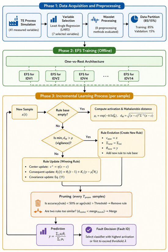
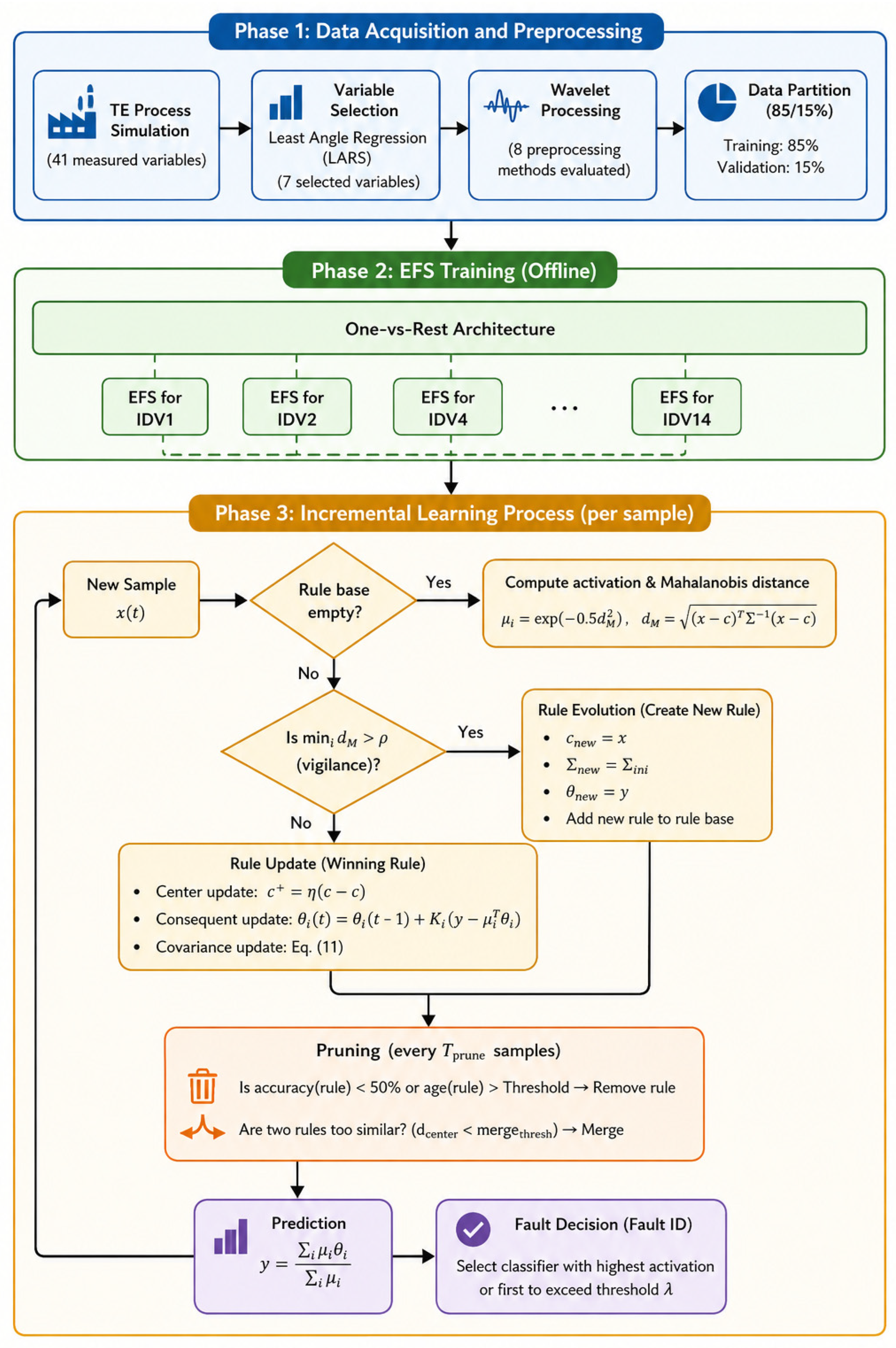
Figure 2 illustrates the proposed EFS-based fault diagnosis framework with wavelet preprocessing. Algorithm 2 shows the same information for programming.

Algorithm 2: Pseudocode for EFS incremental learning in fault detection.

1: Initialize: R = { }, samplecounter = 0

2: for each new sample (x, ytrue) do

3:  samplecounter = samplecounter + 1

4:  if R is empty, then

5:    Create first rule: c1 = x, σ1 = σinit, θ1 = ytrue

6:  else

7:    Compute activations φ1 = exp(−0.5 ∗ dM(i, x)2)

8:    Let i* = argmini dM(i, x)

9:    if dM(i*, x) > ρ and |R| < Rmax, then

10:    Create new rule: cnew = x, σnew = σinit, θnew = ytrue

11:   else

12:    Update winning rule i*: ci* = ci* + η(x − ci*)

13:    Update σi* using rank-one, Equation (11)

14:    Update θi* using RFWLS

15:   end if

16:   if samplecounter mod Tprune == 0, then

17:    Prune rules with (acci < 0.5 or agei > agemax)

18:    Merge rules with ||ci − cj||2 < θmerge and |θi − θj| < θθ

19:   end if

20:  end if

20:  ypred = Σiφnormθi

21:  faultdetected = (ypred > λ)

22: end for

Figure 2. Wavelet-based evolving fuzzy system for fault diagnosis scheme.

3. Results and Discussion

This section presents the experimental results of applying the evolving fuzzy system (EFS) with various preprocessing techniques to the Tennessee Eastman process. We first present the overall effectiveness of conventional preprocessing techniques, and then provide a comparison of wavelet-based methods, followed by a thorough per-fault analysis to identify which faults present the greatest difficulty for the proposed method. Finally, we discuss the implications of the results in light of the current literature.

The EFS itself is deterministic once the training and validation datasets are defined. However, small variations may appear between executions if random data partitioning is employed during the train/validation split stage. In order to improve reproducibility, the same experimental configuration and hyperparameters were maintained throughout all experiments. Another consideration is the pruning stage, because if more fuzzy rules are generated, the results may improve but the interpretability and computational cost will be compromised.

One important characteristic of evolving fuzzy systems is their capability to adapt their rule base incrementally as new data become available. In the proposed framework, incoming samples are processed sequentially without requiring complete retraining of the model structure, allowing the system to evolve its fuzzy rules according to new operating conditions or when data reveal new fault types.

Although, the present work did not explicitly evaluate the incorporation of entirely new fault classes during operation, the evolving architecture provides the structural basis for future adaptive extensions involving unknown or emerging faults under online industrial scenarios. The processed simulated data were added to the EFS to merge fuzzy rules indicting a fault, and with the 15% of data the framework was evaluated to obtain the F1-score.

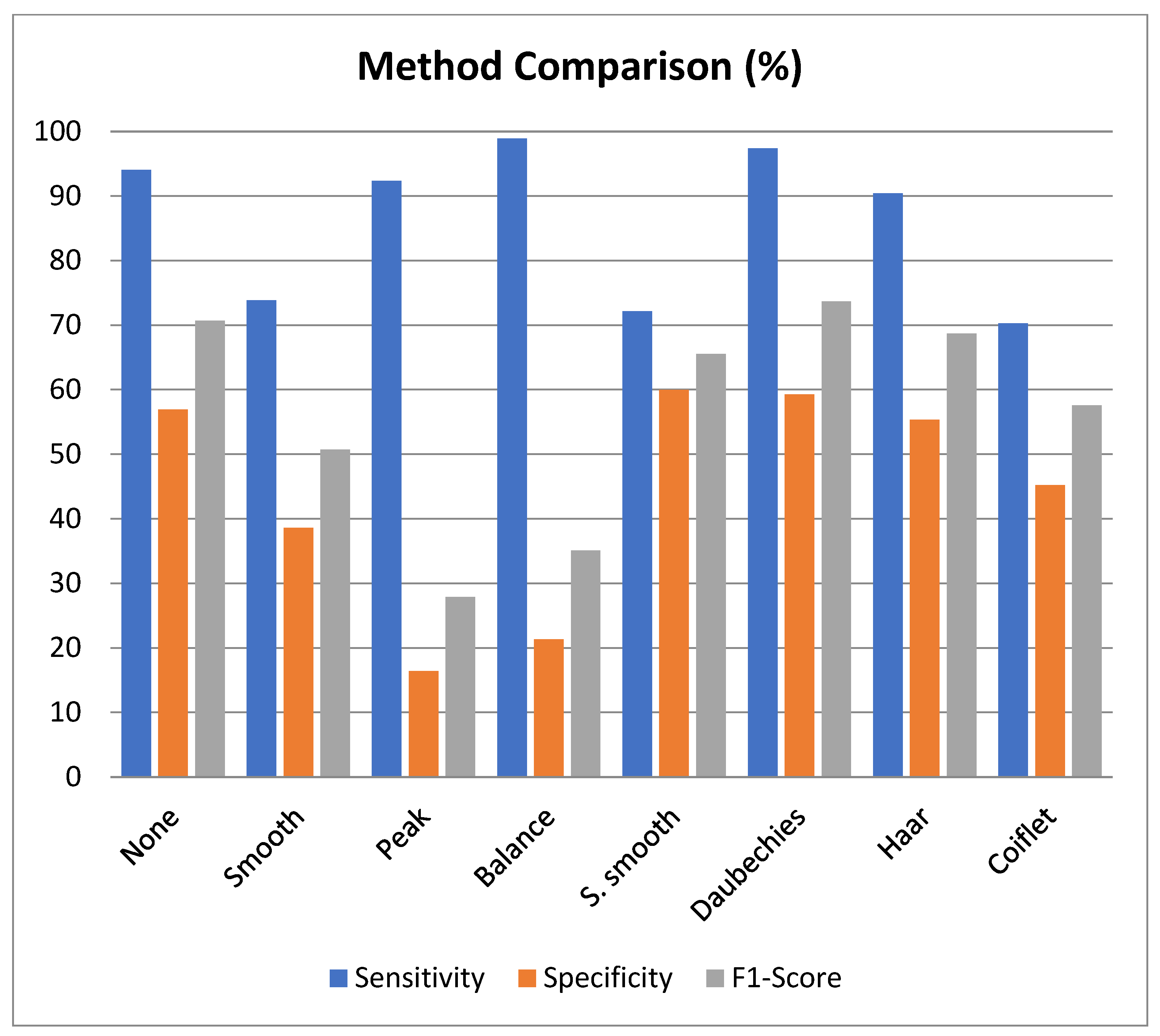
Table 3 shows the performance of five standard preprocessing methods (none, smoothing, peak detection, balanced preprocessing, and strong smoothing) averaged over all ten selected faults. The baseline method (no preprocessing) achieved a sensitivity of 94.03% and an F1-score of 70.67%, setting a standard for comparison. Strong smoothing achieved the highest specificity (59.99%) among conventional methods, but also the lowest sensitivity (72.13%). Balanced preprocessing achieved the highest sensitivity (98.93%) but the lowest specificity (21.33%), indicating a high number of false alarms.

Table 3. Performance of conventional preprocessing methods (averaged over 10 faults).

Method	Sensitivity (%)	Specificity (%)	F1-Score (%)
None (baseline)	94.03	56.93	70.67
Smoothing (window = 3)	73.83	38.60	50.70
Peak detection	92.33	16.43	27.89
Balanced preprocessing	98.93	21.33	35.09
Strong smoothing (window = 7)	72.13	59.99	65.51

3.1. Performance of Wavelet-Based Preprocessing Methods

Table 4 shows the performance of three wavelet-based methods: Haar, Daubechies, and Coiflet wavelets (all at level 4 of decomposition). The Daubechies wavelet method achieved the highest overall F1-score (73.68%) with a sensitivity of 97.37%, substantially outperforming the baseline. The Haar wavelet achieved the best specificity (55.37%) and a competitive F1-score of 68.67%. The Coiflet wavelet, in contrast, performed poorly (F1-score 57.56%), especially on faults IDV1, IDV2, IDV10, and IDV13, where sensitivity dropped to less than 5%.

Table 4. Performance of wavelet-based preprocessing methods (averaged over 10 faults).

Wavelet Method	Sensitivity (%)	Specificity (%)	F1-Score (%)
Daubechies wavelet (level 4)	97.37	59.25	73.68
Haar wavelet (level 4)	90.39	55.37	68.67
Coiflet wavelet (level 4)	79.27	45.19	57.56

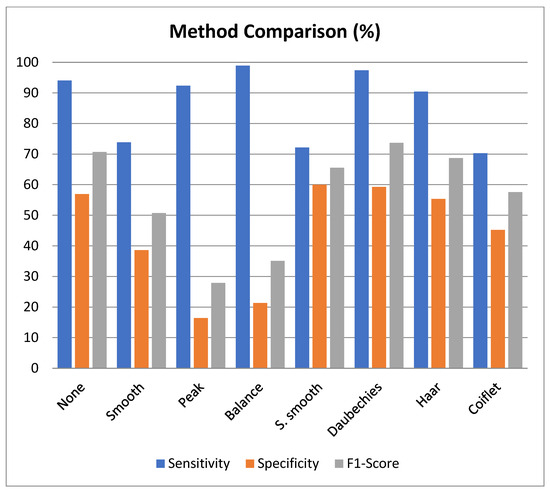
Figure 3 provides a side-by-side comparison of all eight methods tested in this work, including both conventional and wavelet-based methods. The Daubechies and Haar wavelets clearly outperform the others in terms of F1-score, demonstrating the utility of multiscale analysis for fault detection.

Figure 3. Comparative performance of all preprocessing methods.

The lower performance obtained with the Coiflet wavelet may be related to its longer support length and smoother basis functions. Although Coiflets are effective for representing smooth signals with higher regularity [38], several Tennessee Eastman faults produce abrupt transient changes and localized dynamic variations. In such cases, shorter and less smooth wavelets such as Daubechies preserve transient information more effectively.

Furthermore, the fault signatures in the TE process are highly nonstationary and may contain sharp temporal deviations associated with process disturbances. The Coiflet decomposition tends to distribute these local variations across multiple coefficients, reducing class separability in the EFS. This behavior may explain the lower sensitivity and specificity values observed in this approach. Nevertheless, Coiflets may still be useful primarily for incipient faults.

Daubechies wavelets exhibited superior performance due to their compact support and favorable time-frequency localization properties, which allow better preservation of transient fault signatures in nonlinear industrial signals.

Table 5 shows the detailed performance of the Daubechies wavelet method for each of the ten selected faults. The results reveal substantial variation across fault types. IDV4, IDV6, and IDV7 achieved excellent F1-scores (80.80%, 94.89%, and 98.36%, respectively). IDV7 had almost perfect sensitivity (99.67%) and specificity (97.00%).

Table 5. Detailed results for the Daubechies wavelet method per fault.

Fault	Sensitivity (%)	Specificity (%)	F1-Score (%)
IDV1	100.00	54.33	70.40
IDV2	100.00	54.33	70.40
IDV4	99.33	68.10	80.80
IDV5	100.00	54.33	70.40
IDV6	96.00	93.67	94.89
IDV7	99.67	97.00	98.36
IDV8	100.00	54.33	70.40
IDV10	89.45	65.37	75.53
IDV13	93.66	28.66	43.88
IDV14	95.67	45.67	61.83

In contrast, faults IDV1, IDV2, IDV4, IDV5, IDV7, IDV8, and IDV14 have near-100% sensitivity but specificity around 50% (indicating many false alarms). This means the model identified almost all samples as faults in these cases. This behavior suggests that these faults create persistent deviations that are readily identifiable yet challenging to differentiate from normal operation without triggering false alarms (incipient faults).

Faults IDV13 and IDV14 exhibited lower F1-score values compared to the remaining fault classes. Although the proposed framework achieved high sensitivity values above 93% for both cases, specificity remained limited, indicating an increased false alarm rate during classification. This is because IDV13 and IDV14 are known to generate process variations with temporal patterns that partially overlap normal operating fluctuations, making fault discrimination significantly more challenging than for abrupt or highly separable faults. Therefore, the F1-score is an important metric for evaluating framework performance because near-100% sensitivity does not imply an efficient FD scheme.

The evolving fuzzy framework tends to favor conservative detection behavior, maintaining high sensitivity while sacrificing specificity. Although this trade-off increases false alarms, it reduces the probability of missed detections, which is often preferable in safety-critical industrial environments [39].

These results also suggest that additional feature extraction strategies, such as multifractal descriptors, entropy-based measures, or hybrid adaptive thresholds, could further improve discrimination capability for complex incipient faults; this will be a future work.

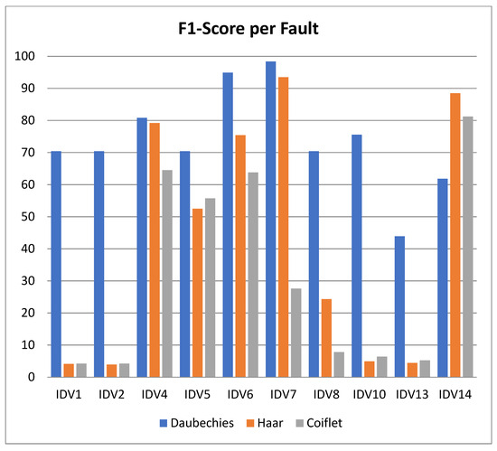
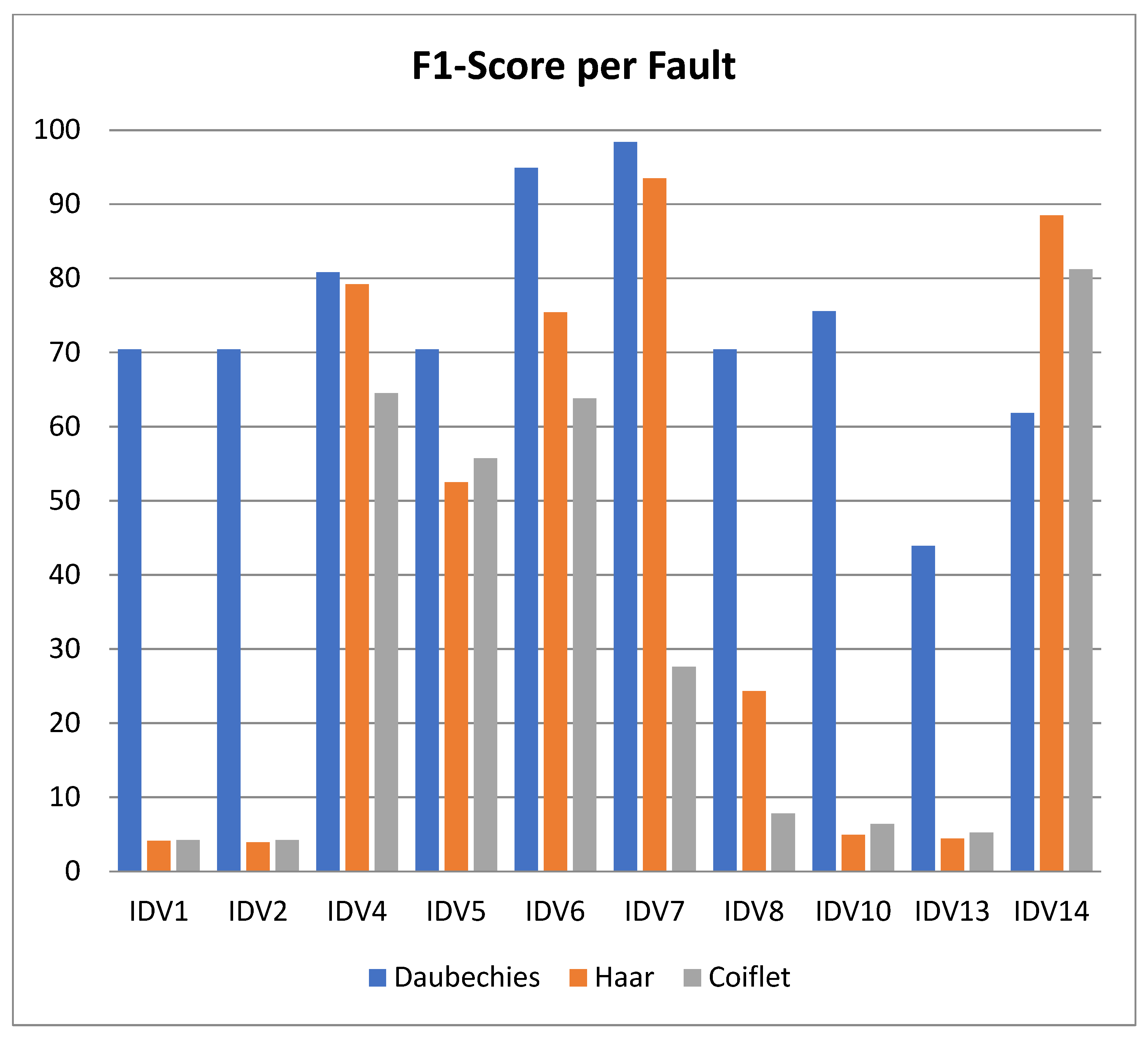
Figure 4 shows the per-fault F1-scores for the three wavelet methods. Most of the time, the Daubechies and Haar wavelets perform similarly across faults. However, Coiflet performs much worse on IDV7, IDV8, and IDV13. This observation suggests that selecting the appropriate wavelet is essential for particular fault types, and no single wavelet is universally superior.

Figure 4. Per-fault F1-score comparison for Daubechies, Haar, and Coiflet wavelets.

Table 6 shows how the best results from this study compare to those found in the literature for the TE process. The Daubechies wavelet method has a sensitivity of 97.37%, which is better than or as good as most other data-driven methods. This performance was achieved with a fully incremental, evolving fuzzy system that does not require retraining when new fault types emerge; a feature absent in static methods. Although deep learning approaches such as LSTM and autoencoders have shown high performance, they require retraining and lack interpretability. An interesting approach to achieving interpretability is given in [40], where a Transformer–LSTM denoising autoencoder achieved competitive fault sensitivities in the TE process through spatiotemporal attention; these results are also compared in Table 6. However, Ref. [40] does not show results for IDV3 because this fault only presents deviations from normal operating conditions.

Table 6. Results comparison among different approaches.

Study	Method	Sesitivity (%)	Notes
Yin et al. [6]	PCA, PLS, ICA	73.8–84.4	Statistical methods (batch)
D’Angelo et al. [32]	Fuzzy clustering + wavelets	88.5	Batch learning, fuzzy logic
Hajihosseini et al. [33]	Wavelets + neural networks	98.6	Requires retraining, black box
Guo et al. [40]	Transformer–LSTM denoising autoencoder	96.50	Semi-supervised, batch learning, requires retraining
Márquez et al. [41]	LSTM + elastic-net	96.45	Deep learning
This approach	EFS + wavelets (one-vs-rest)	97.37	Incremental, no retraining

Compared to deep learning approaches such as Transformer–LSTM models [40], the proposed EFS framework achieves comparable sensitivity while maintaining full interpretability and supporting incremental learning without retraining.

Deep learning methods such as convolutional neural networks (CNNs) and long short-term memory networks (LSTMs) have demonstrated high fault classification performance in industrial processes [41]. However, these approaches usually require extensive training datasets, high computational resources, and retraining procedures when new operating conditions or faults appear.

In contrast, EFSs provide adaptive rule evolution, lower computational complexity, and improved interpretability, making them attractive for industrial applications where transparency and incremental adaptation are required.

3.2. Discussion

The results demonstrate four main findings:

(1)

Wavelet-based preprocessing consistently improves the performance of EFS for FD compared to conventional methods. The Daubechies wavelet achieved the highest F1-score (73.68%) and the best specificity (59.25%).

(2)

The choice of wavelet matters significantly: the Coiflet wavelet underperformed, particularly on faults with abrupt dynamics (e.g., IDV7).

(3)

Certain faults (IDV1, IDV2, IDV5, IDV8) remain challenging, exhibiting high sensitivity but very low specificity. These faults are expected to cause persistent changes in the measured variables that persist even after the fault is removed, making them difficult to distinguish from normal operation without generating false alarms.

(4)

Interestingly, using no preprocessing achieved good sensitivity results, even better than using Haar and Coiflet wavelets to preprocess data for EFS improvement.

From a practical perspective, the selection of preprocessing method should be guided by the specific requirements of the application. If maximizing fault detection (sensitivity) is the priority, for example, in safety-critical systems, the Daubechies wavelet method is recommended for preprocessing. Whereas, if minimizing false alarms (specificity) is more important, for instance, in systems where alarms cause operator fatigue or unnecessary shutdowns, the Haar wavelet method is preferable. Also, in this work we selected the variables that made the most contribution in the signals once a fault is presented. A different set of variables could be chosen for FD. However, some signals present a different behavior when a fault is simulated after some time delay [36].

The window size used for wavelet preprocessing and feature extraction should be selected according to the dominant process dynamics. Small windows increase sensitivity to abrupt changes but may also amplify noise, whereas larger windows provide smoother responses at the expense of slower fault detection.

Additionally, normalization of process variables prior to preprocessing is recommended to avoid dominance of variables with larger amplitudes. The EFS hyperparameters should initially be adjusted using representative operating conditions before deployment in online monitoring scenarios. Although the proposed framework supports adaptive rule evolution, practitioners should periodically inspect newly generated fuzzy rules to determine whether they correspond to novel operating conditions, sensor drift, or genuinely new fault patterns. Such supervision is important to maintain interpretability and to reduce the risk of false alarms during long-term industrial operation.

Several limitations of this study should be acknowledged:

• The evaluation was conducted on simulated data; real-world performance may differ due to unmodeled noise, sensor drift, and other practical factors.
• Only ten of the twenty available TE faults were analyzed; generalization to the remaining faults requires further validation.
• The one-vs-rest architecture, while effective, requires training separate classifiers for each fault, which may become computationally expensive as the number of fault types grows.

Although the TE process is one of the most widely accepted industrial benchmarks for fault diagnosis research, the experiments presented in this work were conducted using simulated data. Therefore, the reported results should be interpreted as a controlled validation of the proposed methodology under representative nonlinear process conditions.

4. Conclusions

This paper showed a comparative study of preprocessing methods for evolving fuzzy systems (EFS) applied to fault diagnosis (FD) in the Tennessee Eastman (TE) process. This work was motivated by the limitations of static fault diagnosis methods, particularly their inability to handle unknown faults and the need for adaptation when process conditions change. This is particularly important when the FD is model-based, when a control action is taken, and the operating point of the system changes over time; in such cases, a static or statistical approach will detect a non-existent fault.

EFS offer a paradigm shift by supporting incremental learning, structural evolution, and parameter adaptation, making them well-suited for adaptive FD applications, principally, when no prior fault information is available.

The main contributions of this work can be summarized in the following way:

• Integration of EFS with wavelet preprocessing. A modular implementation of EFS with one-vs-rest architecture was developed for multi-fault classification. The system processes data incrementally, evolves new fuzzy rules when previously unseen patterns appear, and prunes redundant rules to maintain compactness and interpretability by limiting the number of fuzzy rules.
• Comparative study. Eight preprocessing methods were evaluated to highlight the presence of a fault, and the one with the best result was compared with results reported in the literature.
• Open-source implementation. The codebase was implemented in GNU Octave© to ensure reproducibility.

The Daubechies-4 (db4) wavelet approximation achieved the best overall performance: an F1-score of 73.68% with a sensitivity of 97.37%. The obtained results suggest that multiscale analysis effectively highlights relevant fault signatures in nonlinear industrial process signals. The db4 wavelet achieved the best overall sensitivity and F1-score, whereas the Haar wavelet produced the highest specificity and lowest false alarm rate. However, if no preprocessing is made or a strong smoothing is applied, the sensibility and specificity obtained were 94.03 and 56.93% respectively, but with a lower F1-score.

The one-vs-rest architecture, made here, requires training separate classifiers for each fault. As the number of fault types grows, the computational cost increases linearly. The proposed approach has significantly lower computational complexity compared to deep learning architectures. To maintain stable fault diagnosis performance and preserve interpretability, it is important to control the growth of the fuzzy rule base by pruning redundant or weakly activated rules.

An important advantage of the proposed evolving fuzzy framework is the interpretability of its rule-based structure. Unlike black-box models such as deep neural networks, the evolving fuzzy system generates linguistic fuzzy rules that can be associated with different operating conditions of the process. The number of rules changes dynamically according to the complexity of the monitored data, allowing the model to adapt to new operating regions while maintaining an interpretable structure. In practice, the system typically generates a compact set of rules, which facilitated the analysis of abnormal operating behaviors without requiring complete retraining.

Additionally, the use of wavelet preprocessing contributes to highlighting transient and multiscale characteristics of the process signals before rule generation. Although wavelet coefficients do not always have a direct physical interpretation, they preserve relevant information associated with process dynamics and fault evolution. Consequently, the resulting fuzzy rules can still provide meaningful information regarding changes in process behavior. Nevertheless, as the number of operating conditions and fault classes increases, some overlap between fuzzy premises may appear, which can reduce transparency. For this reason, periodic inspection and pruning of redundant rules may be beneficial in long-term industrial applications.

As industrial processes continue to generate massive streams of data, adaptive, incremental, and interpretable methods like EFS will play an increasingly important role in ensuring safe and efficient operations. This work presents an interpretable and adaptive framework that can be applied when no data history is available, and when an interpretable model is required.

5. Limitations and Future Work

Although the proposed framework demonstrated promising performance in the Tennessee Eastman benchmark, several limitations remain. First, the experiments were conducted using simulated process data rather than measurements obtained from real industrial plants. Consequently, additional validation under real operating conditions is required. Additionally, human supervision may still be required when newly generated fuzzy rules appear, particularly to determine whether they correspond to new operating conditions, sensor drift, or previously unseen fault patterns.

Second, although the evolving fuzzy architecture supports adaptive rule modification, the present study evaluated sequential offline partitions instead of fully online streaming scenarios involving concept drift or dynamic fault incorporation.

Future work will focus on:

• Online adaptive learning;
• Multifractal feature extraction;
• Hybrid entropy–fractal descriptors;
• Using an interpretable framework like Kolmogorov–Arnold networks.

References

- Yimam, A.W.; Vafaeipour, M.; Messagie, M.; Fante, K.A.; Molla, E.M.; Azerefegn, T.M.; Coosemans, T. State-of-the-art of machine learning methods for fault detection and health monitoring of wind turbine system components: A comprehensive review. Eng. Appl. Artif. Intell. 2025, 162, 112645. [Google Scholar] [CrossRef] [Scilit]
- Soleimani, M.; Irani, F.N.; Yadegar, M.; Meskin, N. Comprehensive review of gas turbine fault diagnostic strategies. Appl. Energy 2025, 401, 126801. [Google Scholar] [CrossRef] [Scilit]
- Asmone, A.S.; Goh, Y.M.; Lim, M.S.H. Prioritization of industry level interventions to improve implementation of design for safety regulations. J. Saf. Res. 2022, 82, 352–366. [Google Scholar] [CrossRef] [Scilit] [PubMed]
- Bathelt, A.; Ricker, N.L.; Jelali, M. Revision of the Tennessee Eastman process model. IFAC-PapersOnLine 2015, 48, 309–314. [Google Scholar] [CrossRef] [Scilit]
- Downs, J.J.; Vogel, E.F. A plant-wide industrial process control problem. Comput. Chem. Eng. 1993, 17, 245–255. [Google Scholar] [CrossRef] [Scilit]
- Yin, S.; Ding, S.X.; Haghani, A.; Hao, H.; Zhang, P. A comparison study of basic data-driven fault diagnosis and process monitoring methods on the benchmark Tennessee Eastman process. J. Process Control 2012, 22, 1567–1581. [Google Scholar] [CrossRef] [Scilit]
- Cho, S.; Jiang, J. A fault detection and isolation technique using nonlinear support vectors dichotomizing multi-class parity space residuals. J. Process Control 2019, 82, 31–43. [Google Scholar] [CrossRef] [Scilit]
- Yang, C.; Huang, J.; Wu, S.; Liu, Q. Neural-network-based practical specified-time resilient formation maneuver control for second-order nonlinear multi-robot systems under FDI attacks. Neural Netw. 2025, 186, 107288. [Google Scholar] [CrossRef] [Scilit] [PubMed]
- Cao, X.; Liu, S.; Cen, J. Observer-based adaptive neural asynchronous H∞ Control for fuzzy Markov jump systems under FDI attacks. J. Frankl. Inst. 2024, 361, 107147. [Google Scholar] [CrossRef] [Scilit]
- Lemos, A.; Caminhas, W.; Gomide, F. Adaptive fault detection and diagnosis using an evolving fuzzy classifier. Inf. Sci. 2013, 220, 64–85. [Google Scholar] [CrossRef] [Scilit]
- Schmidt, S.; Gryllias, K.C. An anomalous frequency band identification method utilising available healthy historical data for gearbox fault detection. Measurement 2023, 222, 113515. [Google Scholar] [CrossRef] [Scilit]
- Venkatasubramanian, V.; Rengaswamy, R.; Yin, K.; Kavuri, S.N. A review of process fault detection and diagnosis: Part I: Quantitative model-based methods. Comput. Chem. Eng. 2003, 27, 293–311. [Google Scholar] [CrossRef] [Scilit]
- Lughofer, E. On-line assurance of interpretability criteria in evolving fuzzy systems—Achievements, new concepts and open issues. Inf. Sci. 2013, 251, 22–46. [Google Scholar]
- Kumar, A.A.; Srikumar, D.K.; Rao, D.G.N. A high-dimensional data-driven approach for enhancing cyber-physical attack detection in PV-connected distribution power grids using deep Q-networks. Comput. Electr. Eng. 2026, 129, 110814. [Google Scholar] [CrossRef] [Scilit]
- Lughofer, E.; Pratama, M. Evolving multi-user fuzzy classifier system with advanced explainability and interpretability aspects. Inf. Fusion 2023, 91, 458–476. [Google Scholar] [CrossRef] [Scilit]
- Huang, H.; Rong, H.J.; Yang, Z.X.; Vong, C.M. Jointly evolving and compressing fuzzy system for feature reduction and classification. Inf. Sci. 2021, 579, 218–230. [Google Scholar] [CrossRef] [Scilit]
- Lughofer, E.; Guardiola, C. On-line fault detection with data-driven evolving fuzzy models. Control. Intell. Syst. 2008, 36, 307. [Google Scholar]
- Lughofer, E.; Cernuda, C.; Kinderman, S.; Pratama, M. Generalized smart evolving fuzzy systems. Evol. Syst. 2015, 6, 269–292. [Google Scholar] [CrossRef] [Scilit]
- Pratama, M.; Lu, J.; Zhang, G. Evolving type-2 fuzzy classifier. IEEE Trans. Fuzzy Syst. 2016, 24, 574–589. [Google Scholar]
- Angelov, P.; Filev, D. An approach to online identification of Takagi-Sugeno fuzzy models. IEEE Trans. Syst. Man Cybern. Part B 2004, 34, 484–498. [Google Scholar] [CrossRef] [Scilit] [PubMed]
- Lughofer, E. FLEXFIS: A robust incremental learning approach for evolving Takagi-Sugeno fuzzy models. IEEE Trans. Fuzzy Syst. 2008, 16, 1393–1410. [Google Scholar]
- Kasabov, N.; Song, Q. DENFIS: Dynamic evolving neural-fuzzy inference system and its application for time-series prediction. IEEE Trans. Fuzzy Syst. 2002, 10, 144–154. [Google Scholar] [CrossRef] [Scilit]
- Pratama, M.; Anavatti, S.G.; Angelov, P.P.; Lughofer, E. PANFIS: A novel incremental learning machine. IEEE Trans. Neural Netw. Learn. Syst. 2014, 25, 55–68. [Google Scholar] [CrossRef] [Scilit] [PubMed]
- Pratama, M.; Anavatti, S.G.; Lughofer, E. GENEFIS: Toward an effective localist network. IEEE Trans. Fuzzy Syst. 2014, 22, 547–562. [Google Scholar] [CrossRef] [Scilit]
- Lughofer, E. On Improving Performance and Increasing Useability of EFS. In Evolving Fuzzy Systems—Methodologies, Advanced Concepts and Applications; Springer: Cham, Switzerland, 2011; pp. 213–259. [Google Scholar]
- Lughofer, E. Evolving fuzzy systems: Fundamentals, reliability, interpretability, and applications. In Handbook of Computational Intelligence; World Scientific: Singapore, 2016; pp. 67–135. [Google Scholar]
- Serdio, F.; Lughofer, E.; Pichler, K.; Pichler, M.; Buchegger, T.; Efendic, H. Fuzzy fault isolation using gradient information and quality criteria from system identification models. Inf. Sci. 2015, 316, 18–39. [Google Scholar] [CrossRef] [Scilit]
- Adonovski, G.; Muič, G.; Blažič, S.; Škrjanc, I. Evolving model identification for process monitoring and prediction of non-linear systems. Eng. Appl. Artif. Intell. 2018, 68, 214–221. [Google Scholar] [CrossRef] [Scilit]
- Lughofer, E.; Macián, V.; Guardiola, C.; Klement, E.P. Identifying static and dynamic prediction models for NOx emissions with evolving fuzzy systems. Appl. Soft Comput. 2011, 11, 2487–2500. [Google Scholar] [CrossRef] [Scilit]
- Yan, R.; Gao, R.X.; Chen, X. Wavelets for fault diagnosis of rotary machines: A review with applications. Signal Process. 2014, 96, 1–15. [Google Scholar] [CrossRef] [Scilit]
- Mallat, S. A Wavelet Tour of Signal Processing: The Sparse Way; Academic Press: Cambridge, MA, USA, 2009. [Google Scholar]
- D’Angelo, M.F.S.V.; Palhares, R.M.; Camargos-Filho, M.C.O.; Maia, R.D.; Mendes, J.B.; Ekel, P.Y. A new fault classification approach applied to Tennessee Eastman benchmark process. Appl. Soft Comput. 2016, 49, 676–686. [Google Scholar] [CrossRef] [Scilit]
- Hajihosseini, P.; Anzehaee, M.M.; Behnam, B. Fault detection and isolation in the challenging Tennessee Eastman process by using image processing techniques. ISA Trans. 2018, 79, 137–146. [Google Scholar] [CrossRef] [Scilit] [PubMed]
- He, Y.L.; Zhao, Y.; Hu, X.; Yan, X.N.; Zhu, Q.X.; Xu, Y. Fault diagnosis using novel AdaBoost based discriminant locality preserving projection with resamples. Eng. Appl. Artif. Intell. 2020, 91, 103631. [Google Scholar] [CrossRef] [Scilit]
- Liang, P.; Deng, C.; Wu, J.; Yang, Z.; Zhu, J.; Zhang, Z. Compound fault diagnosis of gearboxes via multi-label convolutional neural network and wavelet transform. Comput. Ind. 2019, 113, 103132. [Google Scholar] [CrossRef] [Scilit]
- Márquez-Vera, M.A.; Ramos-Velasco, L.E.; López-Ortega, O.; Zúñiga-Peña, N.S.; Ramos-Fernández, J.C.; Ortega-Mendoza, R.M. Inverse fuzzy fault model for fault detection and isolation with least angle regression for variable selection. Comput. Ind. Eng. 2021, 159, 107499. [Google Scholar] [CrossRef] [Scilit]
- Chen, J.; Li, Z.; Pan, J.; Chen, G.; Zi, Y.; Yuan, J.; Chen, B.; He, Z. Wavelet transform based on inner product in fault diagnosis of rotating machinery: A review. Mech. Syst. Signal Process 2016, 70, 1–35. [Google Scholar] [CrossRef] [Scilit]
- Mansi, A.; Dunai, L.; Cao, M. Wavelet-based denoising of structural health monitoring strain measurements. Meas. Sens. 2025, 42, 101974. [Google Scholar] [CrossRef] [Scilit]
- Toribio, L.; Veloso, B.; Gama, J.; Zafra, A. A two-stage framework for early failure detection in predictive maintenance: A case study on metro trains. Neurocomputing 2026, 670, 132506. [Google Scholar]
- Guo, L.; Shi, J.; Kang, J.; Li, A. An interpretable Transformer–LSTM denoising autoencoder for semi-supervised fault diagnosis in chemical processes. Eng. Appl. Artif. Intell. 2026, 172, 114358. [Google Scholar] [CrossRef] [Scilit]
- Márquez-Vera, M.A.; López-Ortega, O.; Ramos-Velasco, L.E.; Ortega-Mendoza, R.M.; Fernández-Neri, B.J.; Zúñiga-Peña, N.S. Fault diagnosis using an LSTM and an elastic net. Rev. Iberoam. Autom. Inf. Ind. 2021, 18, 164–175. [Google Scholar]
Disclaimer/Publisher’s Note: The statements, opinions and data contained in all publications are solely those of the individual author(s) and contributor(s) and not of MDPI and/or the editor(s). MDPI and/or the editor(s) disclaim responsibility for any injury to people or property resulting from any ideas, methods, instructions or products referred to in the content. |
© 2026 by the authors. Licensee MDPI, Basel, Switzerland. This article is an open access article distributed under the terms and conditions of the Creative Commons Attribution (CC BY) license.