Strategic Approach for Enhancing Deep Learning Models

Abstract

Modern large language models have achieved remarkable growth and performance across domains, yet their intense use of resources and high computational costs present challenges to scalability and sustainability. Current attempts to surpass baseline (naïve) AutoDL (Automated Deep Learning) models often rely on complex manipulations to yield marginal accuracy gains while demanding deep domain knowledge and computational intensity. To address known inefficiencies in computation and implementation, this study proposes a strategic approach for enhancing processing without compromising model accuracy or performance through a simplified, scalable methodology. We present a novel AutoDL weight optimization model method that analyzes the most accurate deep learning starting point and achieves the highest outcomes while considering the additional “presetting” analysis overhead. Using 20 real-world datasets, we conducted experiments across three models, six weight configurations, and ten seeds, totaling 62,400 epochs. In all experiments, the optimized model outperformed baselines, achieving higher accuracy across every dataset while reducing preprocessing to only two epochs per seed. These results demonstrate that minimal preprocessing—limited to two epochs per seed—can substantially lower computational demand while maintaining precision. As the global demand for AI deployment accelerates, this conservation-oriented approach will be critical to sustaining innovation within resource and infrastructural constraints, enabling advances in computational sustainability and responsible AI development, tangible savings across multiple dimensions of resource consumption, and broader access to deep learning technologies.

1. Introduction

The marked increase in the adoption of artificial intelligence (AI), Machine Learning (ML), and deep learning (DL) methodologies in recent years is evident in the growing number of publications, services, and applications. This upward trend underscores the expanding role of these technologies in addressing complex analytical challenges with greater efficiency, adaptability, and precision across diverse research and practical domains.

Among contemporary methodologies, Artificial Neural Networks (ANNs) have emerged as particularly prominent, being utilized in over 115 studies [1]. While traditional Machine Learning (ML) techniques primarily focus on identifying patterns and making data-driven predictions or decisions, deep learning (DL)—and ANNs in particular—are distinguished by the ability to extract and learn complex features directly from unrefined input data and large databases, It is important to note a recently published study on the subject, which presents a method for reducing the complexity affected by a large number of features [2]. Thus, focusing on these technologies for the development of solutions for a variety of domains, such as health, transportation, finance, education and agriculture, enables smarter, faster, and more adaptive practice for problem-solving [3,4,5,6,7].

By learning from raw data through stacked layers of non-linear transformations, DL eliminates the need for manual feature engineering, enabling more accurate and adaptable solutions. Deep neural networks (DNNs)—the foundational architectures of DL—have been successfully applied across a wide range of disciplines, including image and speech recognition, natural language processing (NLP), autonomous systems, and scientific data analysis. The ability of DL models to capture complex, high-dimensional relationships has driven breakthroughs, particularly in computer vision, speech processing, and, critically, NLP [8,9].

Building on these advancements, recent innovations such as Convolutional Neural Networks (CNNs), as detailed and used in [10] for detecting and transforming raw visual camera data into diagnosis (for agricultural usages), and Recurrent Neural Networks (RNNs) have enabled deep learning systems to automatically extract features and model sequential dependencies—capabilities that laid the groundwork for the development of large language models (LLMs). CNNs introduced hierarchical representation learning, allowing models to capture increasingly abstract features, while RNNs made it possible to preserve contextual information across long sequences, which is an essential property for understanding and generating natural language. Together, these innovations replaced traditional manual feature engineering with end-to-end learning, paving the way for LLMs to achieve near-human-level performance in complex language tasks [11,12].

The next major leap came with the introduction of Transformer-based architectures, which revolutionized LLM deep learning by enabling models to capture long-range dependencies far more effectively than previous sequential models. Modern LLMs such as GPT (https://chatgpt.com/) and BERT (https://ai.google/), comprising billions of parameters, have achieved remarkable results in tasks such as text generation, translation, and reasoning [13]. Their integration into domains like reinforcement learning has assisted in further addressing issues such as sample inefficiency, sparse rewards, and generalization limitations.

However, these powerful models and tools have introduced new concerns, including intense use of resources and high computational costs, factual inconsistencies, inherent biases, and challenges in fine-tuning and generalizing across diverse tasks [14]. With more advanced LLM-based compound AI systems, additional challenges arise, such as prompt sensitivity, difficulty in manual parameter tuning, lack of interpretability, error accumulation, and safety risks, including hallucinations and biased outputs.

To overcome these challenges, recent methods use LLMs as optimizers, incorporating techniques like static and dynamic program analysis, trace propagation, beam search, and Monte Carlo Tree Search (MCTS). These approaches enable efficient prompt and tool refinement without relying on gradient-based optimization, while process supervision and task decomposition help improve interpretability and safety [15].

As LLMs continue to develop in scale and complexity, the models also face practical barriers like high inference latency, increased computational demands, and hardware inefficiencies. Those inefficiencies are especially critical in large-scale deployments with budget and energy constraints. To address these barriers, recent research has proposed strategies such as Quality-aware Cost Optimization (QC-Opt), which predicts output quality to minimize redundant computation, and key and value (KV) cache optimization, which reuses previously computed attention values. Additionally, algorithm-level accelerations (e.g., parallel decoding) and hardware-aware design practices, such as pruning, quantization, and customized compilers like ScaleHLS (Scalable High-Level Synthesis framework) and HIDA (a hierarchical dataflow HLS framework built on ScaleHLS), aim to improve speed and scalability [16,17].

Nevertheless, pre-trained LLMs continue to face challenges in reasoning, alignment to human values, and adaptability across domains. An important advancement in addressing these challenges is post-training language models (PoLMs). Through fine-tuning, alignment via human or AI feedback, efficiency improvements and integration of domain-specific or multi-modal data, PoLMs make LLMs more accurate, adaptable, and compatible with user intent—bridging the gap between general-purpose intelligence and domain-relevant applications [18].

One effective approach to optimizing a neural network’s training, particularly during the initial phases when convergence speed and stability are most critical, is careful weight initialization. Variance-based methods such as Xavier (for symmetric activations) and He initialization (for RELU) are designed to preserve signal magnitude across layers and prevent vanishing or exploding gradients, thereby providing a theoretically sound foundation for effective learning [19]. Another approach, Principal Components-based Initialization (PCsInit), uses PCA (Principal Component Analysis) to initialize the first layer with directions of highest variance in the data, resulting in better-conditioned optimization and faster convergence [20].

To further enhance initialization, data-driven strategies can extract informative patterns directly from the dataset. Methods such as PCA, LDA (Linear Discriminant Analysis), and PLS (Partial Least Squares) generate filters from the training data to initialize convolutional layers, enabling the network to begin learning from meaningful structures instead of noise. This approach enhances generalization and reduces the training burden across various architectures [21]. Reviews of existing strategies also highlight the value of reusing statistical properties or pre-trained weights from related datasets, demonstrating how prior knowledge can optimize the selection of starting weights while shortening training time [22].

The goal of this research is to propose a method to reduce the training time of deep learning models by strategically pre-analyzing model performance. This approach can achieve targeted costs based on user intent—whether for accuracy, classification performance, or F1 score—while minimizing computational effort, such as the number of required epochs. The current deep learning network, particularly during the training phase, demands substantial computational and energy resources; therefore, reducing hardware dependence without sacrificing model precision or output quality represents a highly desirable and significant advancement for both academic research and industrial applications. Achieving such efficiency not only enhances computational sustainability but also broadens accessibility to deep learning technologies across diverse sectors.

This research proposes a strategic approach to Automated Deep Learning (AutoDL) concepts that eliminates the trial-and-error paradigm typically governing model optimization. By demonstrating that an innovative two-epoch pre-analysis stage serves as a high-fidelity signal of long-term performance, the method achieves radical efficiency gains, including validation loss improvements of up to 805% and validation accuracy improvements of up to 21%, without requiring expert-level architectural tuning. This new sophisticated sampling approach to model training transforms AutoML from a resource-intensive overhead into a strategic, scalable filter, effectively establishing a new standard for optimized AI that balances elite computational precision with global environmental and economic sustainability.

2. Methods

2.1. Overview

To address the research goal, we designed a method that identifies the most effective deep learning initialization point through pre-analysis and compares its performance to a standard model trained without such pre-analysis (“regular” baseline) while accounting for the additional computational overhead introduced by the presetting stage.

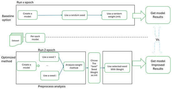
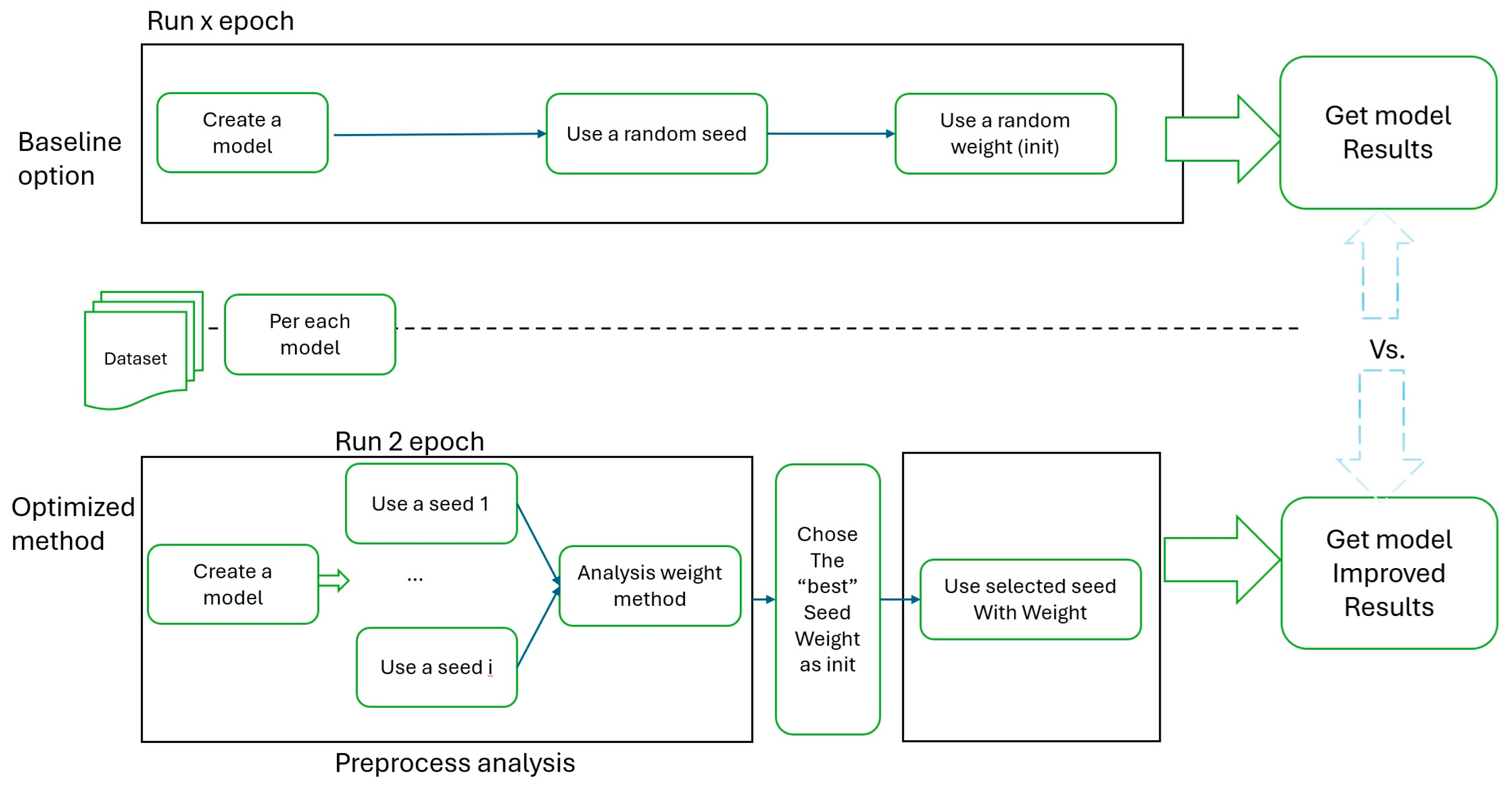
The following diagram (Figure 1) illustrates the high-level method used to implement the research goal, with the baseline option representing the current procedure at a high level.

Figure 1. High-level method.

• Out of three evaluated architectures—SimpleNN, Classifier_Model, and Classifier_CNN_Model—a deep learning model was designed and trained to fit the use case (aka dataset).
• For each run, a designated dataset seed was used to ensure reproducibility.
• Model weights were initialized randomly for the most part, serving as the starting point for training.
• The model ran X epochs until performance metrics, such as a defined confusion matrix value (accuracy, precision, f1 or recall) and/or defined loss values, met predefined thresholds for the use case, or until a maximum of 200 epochs was reached.
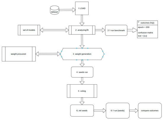
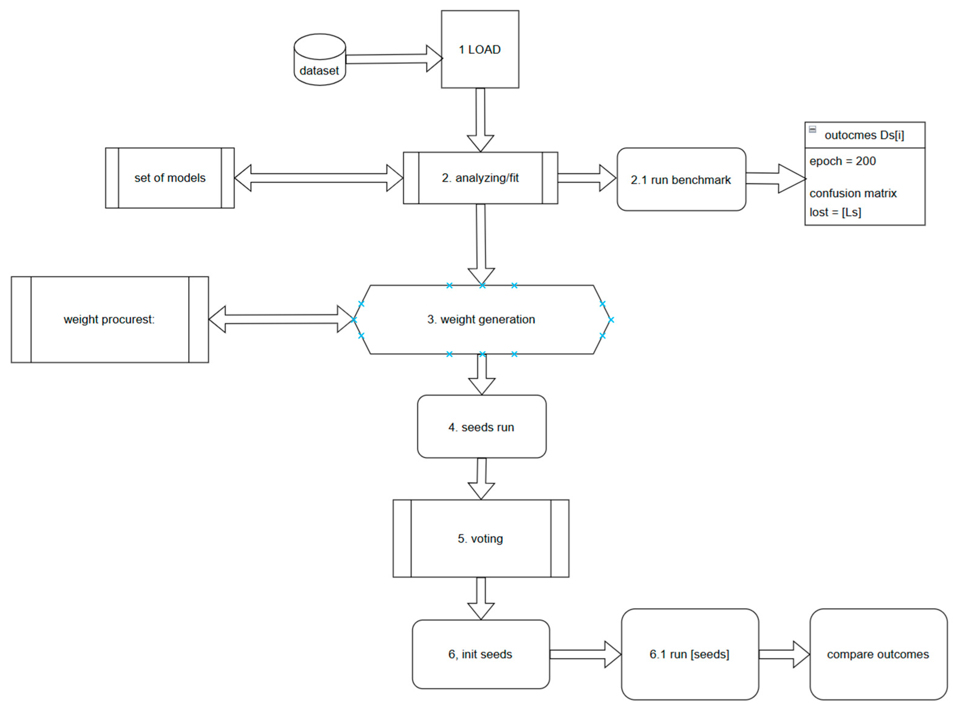
• The first configuration that satisfied the performance condition was recorded as the baseline benchmark for subsequent comparisons, as described at the end of the flow of “get optimal results” compared (vs.) to the model-improved results (see also after step 6.1 in Figure 2).

Figure 2. Detailed method procedures.

The optimized option, as presented at the bottom of Figure 1 (under “Run 2 epoch”) describes the high level of the current procedure as follows:

• A deep learning model (out of the three models) was designed and built to fit the use case (aka dataset) that was examined:
  • Simple NN: A linear model with three layers, fully connected, a hidden layer with 32 nodes, a RELU function, and a dropout rate of 0.3.
  • Classifier_Model: A linear model with three layers, fully connected, a hidden layer with configurable nodes (based on the data features), a RELU function, normalization between the input layer and the hidden layer, and a configurable dropout rate.
  • Classifier_CNN_Model: A model with three convolution layers (Leaky_RELU, maxpool, dropout), flattened, 2 linear layers (Leaky_RELU, dropout), a linear output layer (dropout), and a configurable dropout rate.
• Each model uses a configurable number of seeds. In the research experiment, we used 10 different seeds:
  • Per each seed (i).
  • Analyze six different initial weight methods (Homebrew Normal, Standard Normal, Standard Uniform, Homebrew Uniform, Standard Constant, and Standard Homebrew).
  • Run each seed for two epochs.
• From all seed epoch runs, use the “best” seed results (with the weights) as an initial starting point. Here, “best” seed results = maximum accuracy and minimum loss.
• Run the model with the seeds until the model prediction outcomes are suitable for the use case (up to 200 or until a defined confusion matrix value).

Loop for every weight distribution:

Loop N number of seeds:

Run two epochs and calculate the accuracy value = (TP + TN)/(TP + TN + FP + FN).

If accuracy value > max accuracy:

Update selected seed and random weight method.

$$Accuracy\_value={\displaystyle \frac{1}{Loss\times \left(1-Accuracy\right)+1\times {10}^{-8}}}$$

The final step is to run a full training set using the initial random weight method and seed that produces the highest accuracy value in the best seed procedure.

To describe the internal producers and steps of the designed research methods, Figure 2 presents the end-to-end procedure followed by the explanation in Table 1.

Table 1. Detailed method procedure steps.

#	Name	Description	Note
1	Load	Use case/dataset load to fit in the next step by a DL (deep learning) model	Data preprocessing, such as errors, anomalies, nulls, normalization, types, etc., are out of the scope of this method.
2	Analyzing/fit	Examine a few preconfigured models to analyze and fit the use case	In the model examinations, we used three models: SimpleNN, Classifier_Model, and Classifier_CNN_Model. Note: Can be changed and preconfigured based on needs, requirements, and use cases.
2.1	Baseline run	Run the complete analysis based on the selected seed (42) and random weights	Run up to 200 epochs or until an accuracy value is obtained (the first that answers the condition).
3	Weight generation	Test all weight methods and random seeds as the initial starting point of learning the model	An analysis of six different initial weight methods (Homebrew Normal, Standard Normal, Standard Uniform, Homebrew Uniform, Standard Constant and Standard Homebrew). Note: Can be changed and preconfigured based on needs, requirements, and use cases.
4	Seed run	Run (i) seeds with the weight generation from step 3	In the model examinations, we used i = 10, and each seed ran two epochs. Note: Can be changed and preconfigured based on needs, requirements, and use cases.
5	Voting	Vote between all i seed runs	Analyzing all runs and finding the “best” seeds results + weight as initiated starting point.
6	Init seed	Choose the selected seed and weight from step 5	The selected seed and weight used as the initial step for the full 6.1 run.
6.1	Run (seed)	Outcomes for step 2.1 vs. 6.1	The selected seeds and weight run up to 200 epochs or until an accuracy value is obtained (the first that meets the condition).
	Compare outcomes	Compare outcomes for step 2.1 vs. 6.1	Compare the baseline outcomes vs. the optimized method for a few factors: epoch, accuracy, loss, etc.

Note that both Figure 1 and Figure 2 and the preprocess procedure (Section 2.2) illustrate the high-level main aspects of the model functionalities, while the detailed procedure is presented in the pseudocode section (see Section 2.4).

Table 1 presents the detailed steps shown in Figure 2.

2.2. Preprocess Procedure

The data is preprocessed in the following way:

• The data is downloaded for UC-Irvine using the Python API.
• The data is preprocessed to convert all the input features into numeric, normalized values.
• The data is split into training and validation.
• PyTorch ‘Dataloader’ instances are created for training and validation.

Input features are reprocessed based on their type using the following logic:

• Categorical Features: If a column contains object data types (e.g., strings), it is treated as a categorical feature. The script uses LabelEncoder from scikit-learn to transform the string labels into a numerical format.
• Boolean Features: If a column contains Boolean values, they are converted into integers (True becomes 1; False becomes 0).
• Numeric Features: For columns that are not already numeric, the script attempts to convert them to a numeric type. If any values cannot be converted, they are replaced with the meaning of the column.
• Missing Values: For all numeric columns, any missing values (NaN) are imputed using the meaning of their respective columns. This ensures that the model receives a complete dataset without any missing information.

2.3. Target Features Processing

The target features for the dataset are processed by mapping the target to class values and using classification; the expected output is the prediction of the class.

2.4. Pseudocode

Algorithm 1 below is the detailed formalized pseudocode (as presented and illustrated at a high level in Figure 1 and Figure 2). Note that the full variable and function information is described in the Supplementary Materials file.

Algorithm 1. Detailed method procedure steps.
#	Action
1	Fetch dataset D ← fetch_ucirepo(DatasetName)
2	If dataset size exceeds the limit, truncate D.features and D.targets to MaxDatasetSize
3	Set random seed = 42
4	Organize dataset and create train_loader, val_loader, test_loader
5	Select model M according to ModelType
	If SimpleNN → M ← SimpleNN(input_dim, num_classes)
	If Classifier → M ← Classifier(input_dim, Config.HIDDEN_DIM, num_classes, Config.DROPOUT)
	If TextClassificationModelCnn → M ← TextClassificationModelCnn(input_dim, num_classes, conv_channels, kernel_sizes, dense_layers, dropout_rate)
6	Report model parameters
7	Set loss function C ← CrossEntropyLoss()
8	Set optimizer O (RMSprop or Adam)
9	Configure learning-rate scheduler
	If scheduler enabled → S ← ReduceLROnPlateau(optimizer, mode = “min”, factor = 0.1, patience = 5)
	Otherwise → S ← None
10	Train benchmark model
	loss, acc, epochs ← train_model(M, train_loader, val_loader, C, O, S, Config.NUM_EPOCHS, BenchmarkLoss, TargetAcc)
11	Record benchmark performance
	L_b ← min(loss)
	A_b ← max(acc)
12	Initialize variables
	best_score ← 0
	best_seed ← None
	best_dist ← None
13	Generate random seed → seed ← random(0, 10,000)
14	Apply weight initialization
	apply_random_function_to_weights(M, seed, dist_list[1], Config.training_ratio, dist_list[0])
15	Reset optimizer and loss function
16	Train model for seed evaluation
	loss_s, _, _, acc_s, _ ← train_model(M, train_loader, val_loader, C, O, S, EPOCHS_FOR_BEST_SEED, BenchmarkLoss, TargetAcc)
17	Compute evaluation score
	current_score ← 1/((loss_s[−1] × (1 − acc_s[−1])) + 1 × 10−8)
18	Update best configuration if score improves
	best_score ← current_score
	best_seed ← seed
	best_dist ← dist_list
19	Apply best initialization
	apply_random_function_to_weights(M, best_seed, best_dist[1], Config.training_ratio, best_dist[0])
20	Reset optimizer and loss function
21	Perform final training
	loss_f, acc_f, epochs_f ← train_model(M, train_loader, val_loader, C, O, S, Config.NUM_EPOCHS, L_b, A_b)
22	Evaluate model on test_loader
23	Return summary of benchmark and final metrics

Note: During the research experiment, we used PyTorch [23] library V2.5.1(CPU based) functions; however, the implementation, such as the coding language, environment, data, etc., is out of the scope of this research. Therefore, additional modifications and adjustments may be needed to the coding language, environment, implementation, and data preparation and experiment.

2.5. Model’s Structure

The method (as described in this section) used three different models for each experiment/use case/dataset. Below are the detailed architecture layers of the three selected and examined models:

• SimpleNN = linear, relu, dropout, linear, relu, and linear (six hidden layers).
• Classifier_Model = linear, relu, dropout, relu, normalization, linear, relu, dropout, and linear (9 hidden layers).
• Text_Classifier_Model = linear, leaky_relu, dropout, unsqueeze, convolutional_layer [convolutional, leaky_relu, max_pool, dropout] *(three times), view, dense [linear, leaky_relu, dropout] *(two times), and linear (min 26 layers).

It is important to emphasize that each user/organization can add models, layers, and structures and update them according to their needs, requirements, demands, and so on. The concept of auto-selection between the most suitable seeds, models, and weights will follow the same procedure, with additional parameters and functionalities to choose between (again, depending on the variety of needs).

2.6. Weight Distribution Description

• The weight distribution used in the training of the model was applied using a standard pytorch function from the “pytorch init” library and non-standard (Homebrew) initialization functions that used Python random functions with value manipulation: Standard Normal —“init.normal_()” with a ration divider.
• Standard Uniform—“init.xavier_uniform_()” with a ratio divider.
• Standard Constant—“init.constant_()” with a randomly initialized value.
• Homebrew Normal—Python “randn()” multiplied by the ratio divider.
• Homebrew Uniform—Python “rand()”, where the result is subtracted by 0.5, and the entire value is multiplied by the ratio divider.
• Homebrew constant—Fill all the parameters with a random value between 0 and 1.

2.7. Examined Datasets

For each of the 20 datasets, we ran each of the three models (with and without a scheduler) using six weights and ten seeds and then performed a final test of 200 epochs on the selected test set. A total of 62,400 epochs were experimented with and tested during this research.

3. Results and Analysis

It is important to note that the implementation of the fully described method (see the pseudocode) can be achieved in various environments, coding languages, and designated tools, as well as tailored to different user needs and requirements (including additional parameters and demands); therefore, the fully described method falls outside the scope of this paper.

The following section presents the datasets used to explore, test, and verify the implemented method. Table 2 shows the details of the experiment datasets that were used for this research, which include different features as inputs to the model.

Table 2. Experiment dataset index.

Index/Dataset Name	Info (Features, Records, Reference)
1/Abalone	#features: 8, #records: 4177, [24]
2/Adult	#features: 14, #records: 48,842, [25]
3/Balance Scale	#features: 4, #records: 625 [26]
4/Bank Marketing	#features: 16, #records: 45,211, [27]
5/Breast Cancer	#features: 9, #records: 286 [28]
6/Car Evaluation	#features: 6, #records: 1728 [29]
7/CDC Diabetes Health Indicators	#features: 21, #records: 253,680 [30]
8/Census Income	#features: 14, #records: 48,842 [31]
9/Default of Credit Card Clients	#features: 23, #records: 30,000 [32]
10/Dry Bean	#features: 16, #records: 13,611 [33]
11/Estimation of Obesity Levels Based On Eating Habits and Physical Condition	#features: 16, #records: 2111 [34]
12/Letter Recognition	#features: 16, #records: 20,000 [35]
13/National Poll on Healthy Aging	#features: 14, #records: 714 [36]
14/Nursery	#features: 8, #records: 12,960 [37]
15/Online News Popularity	#features: 58, #records: 39,797 [38]
16/Online Shoppers Purchasing Intention Dataset	#features: 17, #records: 12,330 [39]
17/Statlog	#features: 20, #records: 1000 [40]
18/Student Dropout	#features: 36, #records: 4424 [41]
19/Toxicity	#features: 1203, #records: 171 [42]
20/Wine Quality	#features: 11, #records: 4898 [43]

Note: For the efficiency of the experiment, we used only the first 8000 records (configurable parameters). The index values for the datasets are used throughout the Results Section (graphs and tables).

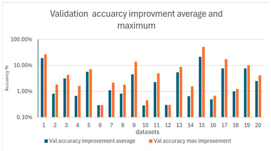
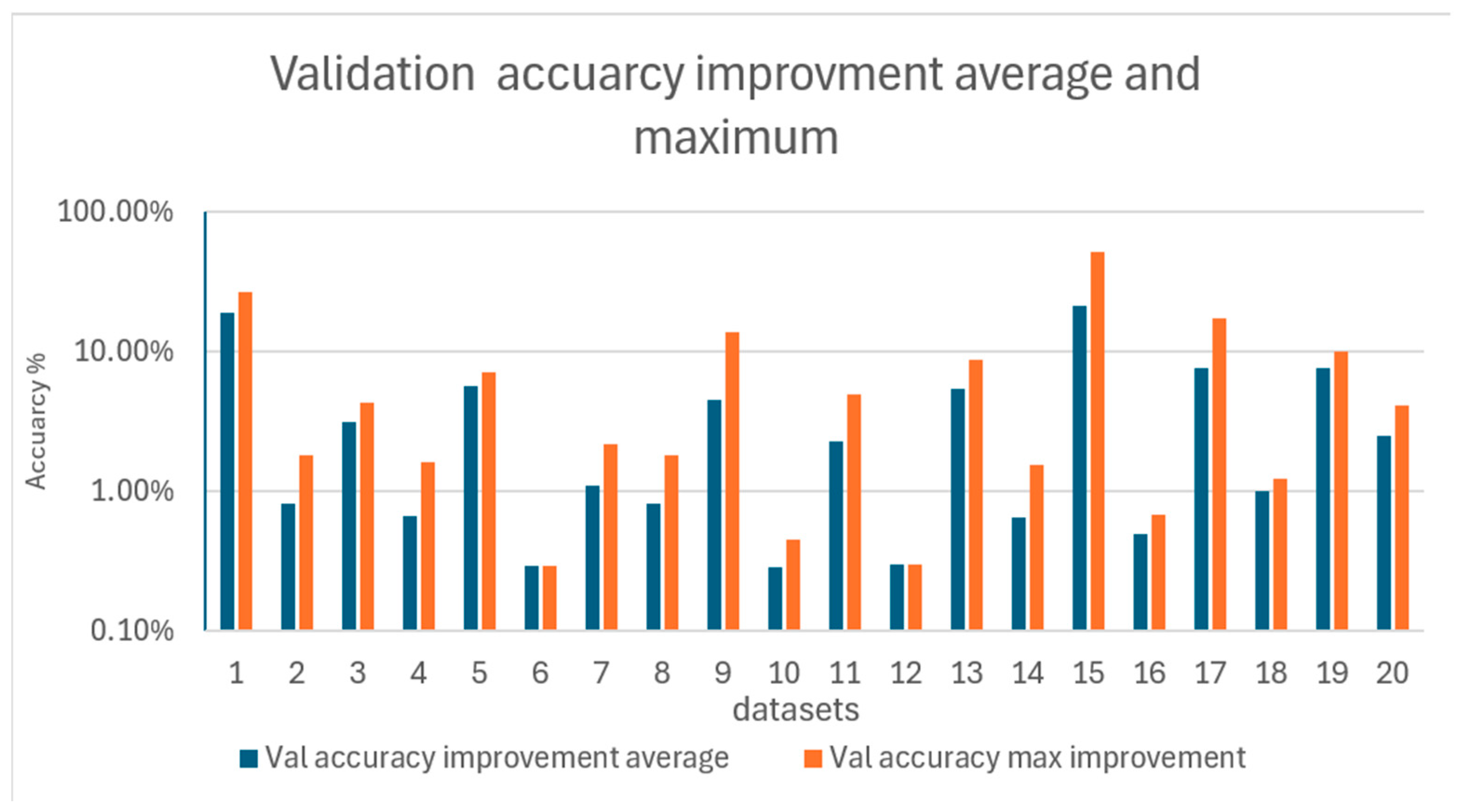
Below, Figure 3 presents the complete run analysis of the model on the 20 databases (index value of axis X represents the dataset index described in Algorithm 1: experiment dataset). As presented in the diagram, all datasets achieve improvements, as illustrated by the maximum accuracy outcomes (26.67%% in dataset 1, 51.56% in dataset 6, etc.). The values in the figure are presented in Table S3.

Figure 3. List of dataset average and maximum validation accuracy improvements.

Figure 3 shows the validation accuracy improvement, both average and maximum, for each dataset in successful experiments on model training and validation. The figure shows logarithmic values, and the graph indicates that the proposed approach yields higher accuracy.

Table 3 describes the average and maximum validation accuracy improvements for each dataset. As presented, the model achieves a better accuracy (compared to the baseline) in all experiments modeled on the 20 datasets.

Table 3. Validation accuracy improvement: average and maximum.

Dataset ID	Validation Accuracy Improvement Average	Validation Accuracy Max Improvement
1	18.96%	26.67%
2	0.81%	1.81%
3	3.06%	4.24%
4	0.66%	1.60%
5	5.60%	6.98%
6	0.29%	0.29%
7	1.08%	2.14%
8	0.81%	1.81%
9	4.48%	13.66%
10	0.29%	0.45%
11	2.23%	4.90%
12	0.30%	0.30%
13	5.30%	8.70%
14	0.64%	1.53%
15	21.04%	51.56%
16	0.49%	0.67%
17	7.50%	17.05%
18	0.98%	1.20%
19	7.50%	10.00%
20	2.44%	4.11%

Note: The full experimental outcomes in Table 3, including the baseline and model outcomes, per dataset, are presented in Table S1.

Based on the full outcomes (see Table S1), the Wilcoxon Signed-Rank test was used to assess whether the median difference between paired observations, the accuracy baseline, and the accuracy model differs significantly from zero.

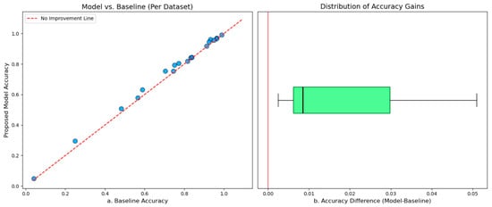
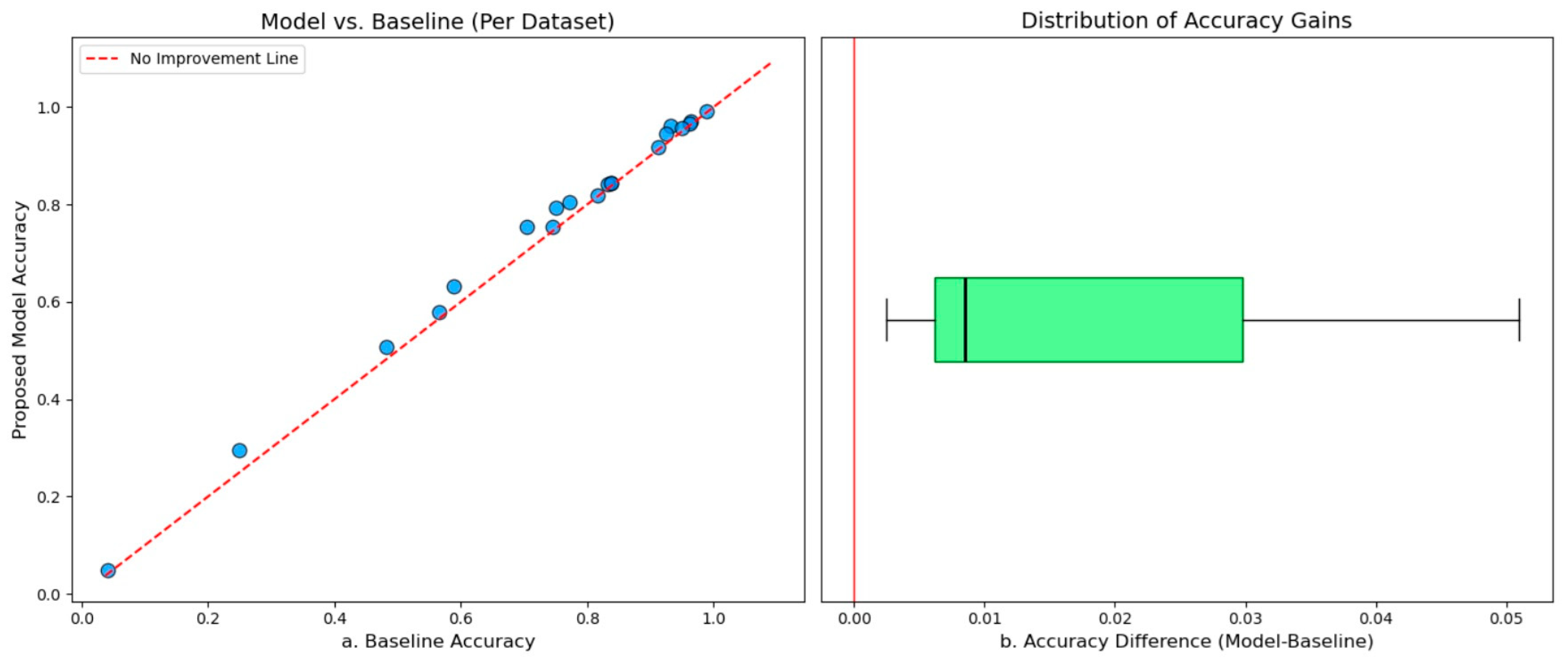
As shown in Figure 4, left, most of the model’s outcomes lie above the identity line, indicating consistent improvement over the baseline. This visual evidence supports the statistical significance found in our analysis. The boxplot on the right illustrates the distribution of net accuracy gains, showing that the majority of the improvements are concentrated well above the zero axis, which confirms the robustness of the proposed model.

Figure 4. Performance comparison between the model and baseline. (a) Individual dataset accuracy comparison. (b) Distribution of accuracy gains showcasing a consistent positive shift.

A statistical analysis of the experimental results across 20 datasets demonstrates a clear and significant performance advantage for the proposed model. Utilizing the Wilcoxon Signed-Rank test, we observed a highly significant improvement (p = 4.42245751 × 10⁻⁵), with the model reaching a mean accuracy of 76.13% compared to the baseline’s 74.30%. This represents a consistent average gain of 1.83 percentage points. Furthermore, the 95% confidence interval for this improvement ranges from 1.05% to 2.61%, confirming that the performance enhancement is robust and statistically distinguishable from zero. These findings provide strong evidence that the proposed method yields a reliable and systematic increase in predictive accuracy.

Table 3 below presents the complete run analysis of the model across 20 databases for loss improvement. As presented, all datasets achieve improvements, as illustrated by the average accuracy outcomes (up to 805% in dataset 19). Furthermore, Table 3 shows the validation loss improvement, both average and maximum, for each dataset across successful model training and validation experiments. The figure shows logarithmic values, and the graph indicates that the proposed approach yields lower loss values. Furthermore, Table 4 describes the average and maximum validation loss improvements for each dataset. The model achieves improved loss values (compared to the baseline) for all 20 datasets and experiments.

Table 4. Validation loss improvement: average and maximum.

Dataset ID	Validation Loss Improvement Average	Validation Loss Max Improvement
1	62.16%	121.88%
2	28.58%	127.17%
3	103.81%	361.87%
4	777.06%	2175.11%
5	129.67%	568.84%
6	13.36%	13.36%
7	7.12%	17.79%
8	28.58%	127.17%
9	31.59%	118.09%
10	21.12%	65.47%
11	21.74%	50.57%
12	0.64%	0.64%
13	183.33%	540.15%
14	38.03%	115.20%
15	44.16%	188.71%
16	113.77%	312.75%
17	448.09%	2130.73%
18	17.87%	28.38%
19	805.68%	1489.62%
20	1.51%	2.08%

In addition to standard cross-validation metrics such as accuracy and loss, which are commonly employed to assess model reliability and quantify uncertainty, we also evaluated the model’s capacity for resource optimization. This assessment was based on measuring the number of epochs required to reach predefined success criteria, defined as follows:

• The validation accuracy in the test run exceeds the benchmark (baseline) validation accuracy.
• The validation loss in the test run is lower than the benchmark validation loss.
• The final epoch count corresponds to the point at which both criteria (1) and (2) are simultaneously satisfied.

This approach allowed us to assess not only the model’s predictive performance but also its computational efficiency, highlighting potential reductions in training time and resource consumption.

It is important to note that the model operates in two configurations (as described in the Passcode): with or without a scheduler. The scheduler enables early termination of training when no further improvement in performance is observed.

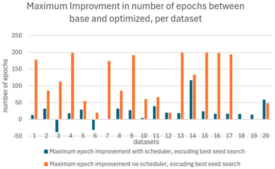
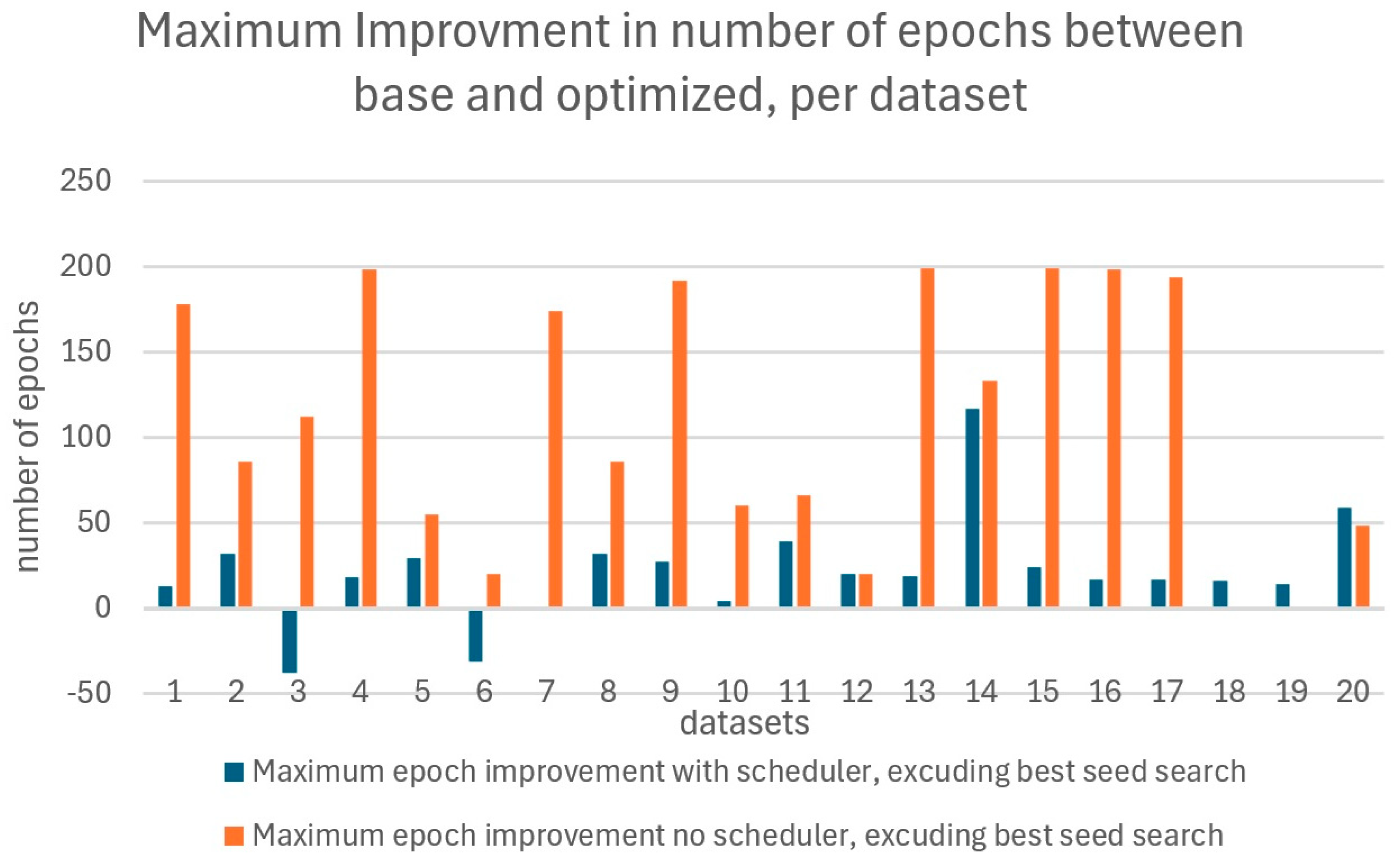
Figure 5 presents the maximum improvement in the number of epochs between the baseline and optimized models for each dataset. As shown in Figure 5, across all 20 experimental datasets, the model achieves at least one maximum improvement, both with and without a learning rate scheduler. The values (as shown in Table 4) are the number of improved approaches compared to the baseline for each dataset. It is important to note that the maximum number of epochs per dataset is chosen from 180 different results per dataset (as described in the method) per schedule/non-schedule run:

$$10 seeds\times 6 random weighted distribution\times 3 models=180$$

Figure 5. Maximum improvement in the number of epochs between base and optimized, per dataset.

Figure 5 shows the best improvement in the number of epochs required to achieve the baseline accuracy and loss target for each dataset across successful model training and validation experiments. The graph indicates that the proposed approach reduces the maximum number of epochs required to achieve baseline accuracy and loss on the majority of datasets.

Table 5 describes the improvement in the epoch maximum value for each dataset. It is essential to emphasize that the table values already include the “overhead” of two epochs per ten seeds analysis (as presented in Section 2), so each value, including an additional 20-epoch “overhead,” and the maximum epoch improvement, is better compared to the baseline.

Table 5. Maximum improvement in the number of epochs between base and optimized, per dataset.

Dataset ID	Maximum Epoch Improvement with Scheduler, Excluding Best Seed Search	Maximum Epoch Improvement NO Scheduler, Excluding Best Seed Search
1	13	178
2	32	86
3	−38	112
4	18	198
5	29	55
6	−31	20
7	−1	174
8	32	86
9	27	192
10	4	60
11	39	66
12	20	20
13	19	199
14	117	133
15	24	199
16	17	198
17	17	194
18	16	0
19	14	0
20	59	48

The data in Table 5, displaying the maximum improvement for each dataset, is a result of testing all the models and the seeds in the datasets, and summing up each dataset. Three models were tested with six weight distributions, along with ten different seeds per weight distribution. As the number of epochs was reduced, the model’s training costs decreased. Research [44] proposes reducing the energy required for model training to achieve Green AI by reducing the complexity of the deep learning network (with additional producers). Issues regarding energy consumption, GPU, and consumption analysis are out of scope for this research and should be subject to future research.

Additional experiments should focus on the performance of resource improvements to demonstrate and determine the conditions, as well as possibly predict the epoch increment, across different use cases, datasets, and requirements. Moreover, additional research is needed for developing model prediction, based on AI functionality, to determine if a dataset may be a suitable candidate for the model.

4. Conclusions and Discussion

This study introduces a strategic, scalable method for enhancing computational efficiency in deep learning without compromising model accuracy or performance. By integrating a lightweight pre-analysis stage within the AutoDL architecture, the method sustains—or even improves—model outcomes while requiring substantially fewer computational resources.

Existing attempts to improve baseline (naïve) AutoDL models often depend on intricate adjustments, such as alternative weight initializations, multiple model architectures, or extensive seed variations. Although these methods can yield marginal improvements, they demand significant domain expertise and computational power. In contrast, our approach offers a simplified, scalable methodology that emphasizes efficiency in both computation and implementation.

The findings demonstrate that limiting pre-analysis to only two epochs per seed can markedly reduce processing time and resource use while maintaining precision. This optimization generates measurable savings in processor load, memory usage, energy consumption, cooling requirements, and overall operational cost. As global demand for AI deployment continues to climb, such conservation-oriented approaches will be critical to sustaining innovation within resource and infrastructure constraints.

The method used in this research presents impressive improvements in the validation accuracy analysis of dozens of percentages, such as 21% in the case of dataset 15, or almost 19% (18.96) in the case of dataset 1. In the case of the validation loss improvement average analysis, in some cases, we observed hundreds of percentages of enhancements, such as 805% in dataset 19, 777% in dataset 4, etc.

Furthermore, as presented in this research, all experiments across all 20 datasets show improvement in the number of maximum epochs (with or without a scheduler).

Beyond immediate computational savings, the framework presented here enables broader organizational flexibility. Reducing energy and hardware demands allows for redirecting existing resources toward parallel research or deployment activities, thereby fostering both economic and environmental sustainability. The method’s modular design also allows adaptation to different user needs, datasets, and service requirements, enabling dynamic optimization based on contextual priorities.

Future research should evaluate this resource-efficient strategy on additional datasets and application domains to further validate its robustness and scalability. Widespread integration of this approach into diverse AI infrastructures could meaningfully advance the emerging field of sustainable artificial intelligence, balancing high performance with responsible resource stewardship. Furthermore, additional models and DL architectures, such as RNNs, CNNs, and Transformers, can be explored and/or combined to improve outcomes, adapt the model to additional use cases, and make it more flexible and adaptable across a variety of services.

References

- Tapeh, A.T.G.; Naser, M.Z. Artificial intelligence, machine learning, and deep learning in structural engineering: A scientometrics review of trends and best practices. Arch. Comput. Methods Eng. 2023, 30, 115–159. [Google Scholar] [CrossRef] [Scilit]
- Gutman, D.; Perel, N.; Bărbulescu, O.; Koren, O. A hybrid dimensionality reduction procedure integrating clustering with KNN-based feature selection for unsupervised data. Algorithms 2025, 18, 188. [Google Scholar] [CrossRef] [Scilit]
- Scheetz, J.; Rothschild, P.; McGuinness, M.; Hadoux, X.; Soyer, H.P.; Janda, M.; Condon, J.J.J.; Oakden-Rayner, L.; Palmer, L.J.; Keel, S.; et al. A survey of clinicians on the use of artificial intelligence in ophthalmology, dermatology, radiology and radiation oncology. Sci. Rep. 2021, 11, 5193. [Google Scholar] [CrossRef] [Scilit]
- Iyer, L.S. AI enabled applications towards intelligent transportation. Transp. Eng. 2021, 5, 100083. [Google Scholar] [CrossRef] [Scilit]
- Fares, O.H.; Butt, I.; Lee, S.H.M. Utilization of artificial intelligence in the banking sector: A systematic literature review. J. Financ. Serv. Mark. 2023, 28, 835–852. [Google Scholar] [CrossRef] [Scilit]
- Chen, L.; Chen, P.; Lin, Z. Artificial intelligence in education: A review. IEEE Access 2020, 8, 75264–75278. [Google Scholar] [CrossRef] [Scilit]
- Nautiyal, N.; Joshi, S.; Hussain, I.; Rawat HJoshi, A.; Saini, A.; Kapoor, R.; Verma, H.; Nautiyal, A.; Chikara, A.; Ahmad, W.; et al. Revolutionizing agriculture: A comprehensive review on artificial intelligence applications in enhancing properties of agricultural produce. Food Chem. 2025, 29, 102748. [Google Scholar] [CrossRef] [Scilit]
- Janiesch, C.; Zschech, P.; Heinrich, K. Machine learning and deep learning. Electron. Mark. 2021, 31, 685–695. [Google Scholar] [CrossRef] [Scilit]
- Alzubaidi, L.; Zhang, J.; Humaidi, A.J.; Al-Dujaili, A.; Duan, Y.; Al-Shamma, O.; Santamaría, J.; Fadhel, M.A.; Al-Amidie, M.; Farhan, L. Review of deep learning: Concepts, CNN architectures, challenges, applications, future directions. J. Big Data 2021, 8, 74. [Google Scholar] [CrossRef] [Scilit]
- Ali, S.; Hassan, M.; Saleem, M.; Tahir, S.F. Deep transfer learning-based hepatitis B virus diagnosis using spectroscopic images. Int. J. Imaging Syst. Technol. 2021, 31, 94–105. [Google Scholar] [CrossRef] [Scilit]
- LeCun, Y.; Bengio, Y.; Hinton, G. Deep learning. Nature 2015, 521, 436–444. [Google Scholar] [CrossRef] [Scilit]
- Shrestha, A.; Mahmood, A. Review of deep learning algorithms and architectures. IEEE Access 2019, 7, 53040–53065. [Google Scholar] [CrossRef] [Scilit]
- Shao, M.; Basit, A.; Karri, R.; Shafique, M. Survey of different large language model architectures: Trends, benchmarks, and challenges. IEEE Access 2024, 12, 188664–188706. [Google Scholar] [CrossRef] [Scilit]
- Cao, Y.; Zhao, H.; Cheng, Y.; Shu, T.; Chen, Y.; Liu, G.; Liang, G.; Zhao, J.; Yan, J.; Li, Y. Survey on large language model-enhanced reinforcement learning: Concept, taxonomy, and methods. IEEE Trans. Neural Netw. Learn. Syst. 2024, 36, 9737–9757. [Google Scholar] [CrossRef] [Scilit] [PubMed]
- Lin, M.; Sheng, J.; Zhao, A.; Wang, S.; Yue, Y.; Wu, Y.; Liu, H.; Liu, J.; Huang, G.; Liu, Y.-J. LLM-based optimization of compound AI systems: A survey. arXiv 2024, arXiv:2410.16392. [Google Scholar] [CrossRef] [Scilit]
- Shekhar, S.; Dubey, T.; Mukherjee, K.; Saxena, A.; Tyagi, A.; Kotla, N. Towards optimizing the costs of LLM usage. arXiv 2024, arXiv:2402.01742. [Google Scholar] [CrossRef] [Scilit]
- Huang, Y.; Wan, L.J.; Ye, H.; Jha, M.; Wang, J.; Li, Y.; Zhang, X.; Chen, D. New solutions on LLM acceleration, optimization, and application. In Proceedings of the 61st ACM/IEEE Design Automation Conference, San Francisco, CA, USA, 23–27 June 2024; pp. 1–4. [Google Scholar]
- Tie, G.; Zhao, Z.; Song, D.; Wei, F.; Zhou, R.; Dai, Y.; Yin, W.; Yang, Z.; Yan, J.; Su, Y.; et al. A survey on post-training of large language models. arXiv 2025, arXiv:2503.06072. [Google Scholar] [CrossRef] [Scilit]
- Kumar, S.K. On weight initialization in deep neural networks. arXiv 2017, arXiv:1704.08863. [Google Scholar] [CrossRef] [Scilit]
- Phan, N.; Nguyen, T.; Halvorsen, P.; Riegler, M.A. Principal components for neural network initialization. arXiv 2025, arXiv:2501.19114. [Google Scholar] [CrossRef] [Scilit]
- Narkhede, M.; Mahajan, S.; Bartakke, P. Data-driven weight initialization strategy for convolutional neural networks. Evol. Intell. 2025, 18, 1. [Google Scholar] [CrossRef] [Scilit]
- Narkhede, M.V.; Bartakke, P.P.; Sutaone, M.S. A review on weight initialization strategies for neural networks. Artif. Intell. Rev. 2022, 55, 291–322. [Google Scholar] [CrossRef] [Scilit]
- Paszke, A.; Gross, S.; Massa, F.; Lerer, A.; Bradbury, J.; Chanan, G.; Killeen, T.; Lin, Z.; Gimelshein, N.; Antiga, L.; et al. PyTorch: An Imperative Style, High-Performance Deep Learning Library. arXiv 2019, arXiv:1912.01703. [Google Scholar]
- Nash, W.; Sellers, T.; Talbot, S.; Cawthorn, A.; Ford, W. Abalone [Dataset]; UCI Machine Learning Repository. 1994. Available online: https://archive.ics.uci.edu/dataset/1/abalone (accessed on 26 March 2026). [CrossRef]
- Becker, B.; Kohavi, R. Adult [Dataset]; UCI Machine Learning Repository. 1996. Available online: https://archive.ics.uci.edu/dataset/2/adult (accessed on 26 March 2026). [CrossRef]
- Siegler, R. Balance Scale [Dataset]; UCI Machine Learning Repository. 1976. Available online: https://archive.ics.uci.edu/dataset/12/balance+scale (accessed on 26 March 2026). [CrossRef]
- Moro, S.; Rita, P.; Cortez, P. Bank Marketing [Dataset]; UCI Machine Learning Repository. 2014. Available online: https://archive.ics.uci.edu/dataset/222/bank+marketing (accessed on 26 March 2026). [CrossRef]
- Zwitter, M.; Soklic, M. Breast Cancer [Dataset]; UCI Machine Learning Repository. 1988. Available online: https://archive.ics.uci.edu/dataset/14/breast+cancer (accessed on 26 March 2026). [CrossRef]
- Bohanec, M. Car Evaluation [Dataset]; UCI Machine Learning Repository. 1988. Available online: https://archive.ics.uci.edu/dataset/19/car+evaluation (accessed on 26 March 2026). [CrossRef]
- CDC. Diabetes Health Indicators [Dataset]; UCI Machine Learning Repository. 2020. Available online: https://archive.ics.uci.edu/dataset/891/cdc+diabetes+health+indicators (accessed on 26 March 2026). [CrossRef]
- Kohavi, R. Census Income [Dataset]; UCI Machine Learning Repository. 1996. Available online: https://archive.ics.uci.edu/dataset/20/census+income (accessed on 26 March 2026). [CrossRef]
- Yeh, I. Default of Credit Card Clients [Dataset]; UCI Machine Learning Repository. 2009. Available online: https://archive.ics.uci.edu/dataset/350/default+of+credit+card+clients (accessed on 26 March 2026). [CrossRef]
- Dry Bean [Dataset]; UCI Machine Learning Repository. 2020. Available online: https://archive.ics.uci.edu/dataset/602/dry+bean+dataset (accessed on 26 March 2026). [CrossRef]