A Century of General Lichtenecker Equation: Between Stringency and Empiricism, Accuracy and Approximability

Abstract

The general Lichtenecker equation, with exponent values in the range $-1\le k\le 1$, is widely used to describe and predict the effective macroscopic electrical, magnetic, thermal and optical properties of various heterogeneous media. Although it sometimes fits experimental data well, in most cases, however, it is physically incorrect and its predictive ability is often overestimated. Using a rigorous spectral representation, we show that for isotropic composites, except for the trivial one-dimensional case, only two specific forms of this equation, the logarithmic ($k=0$) and Landau-Lifshitz-Looyenga ($k=1/3$) mixing laws, are dimensionally consistent, corresponding to spatial dimensions $d=2$ and $d=3$, respectively. Furthermore, the requirement of phase-interchange symmetry severely restricts the applicability of the Lichtenecker equation, rendering it unsuitable for most real composite systems.

1. Introduction

Many researchers and engineers face the problem of expressing the effective macroscopic response (such as permittivity, conductivity, diffusivity, etc.) of various heterogeneous media, including dielectric composites, porous materials, disordered systems. Perhaps the most popular approach is based on phenomenological effective medium (homogenization) theories. Three of them, associated with the names of Maxwell Garnett, Bruggeman and Lichtenecker, are especially frequently used.

In 2026, it is a century as Karl Lichtenecker first put forward his empirical mixing rules [1]. The original equation for the effective permittivity ${ϵ}_{eff}$ in its general form was

$${ϵ}_{eff}^k=f_1{ϵ}_1^k+f_2{ϵ}_2^k,$$

(1)

where $f_1$ and $f_2$ are the volume fractions of the phases 1 and 2, respectively, ${ϵ}_1$ and ${ϵ}_2$ are their permittivities, and k is a phenomenoligical parameter. The value of k in Equation (1) is constrained by the Wiener bounds, i.e., $-1\le k\le 1$, and is often considered as a fitting parameter.

In his earlier paper [2], Lichtenecker also proposed an equation of the form

$$\log \left({ϵ}_{eff}\right)=f_1\log \left({ϵ}_1\right)+f_2\log \left({ϵ}_2\right),$$

(2)

which can in fact be considered as a particular case of Equation (1) in the limit $k\to 0$. The main assumption made in deriving Equation (2) is a random distribution of particle shapes and orientations for each phase such that the charge density within any phase can be replaced by the mean charge density of the mixture. This allows one to replace the charge fractions with their volume fractions [3].

In the literature, Equation (2) is also frequently called as Lichtenecker equation. To avoid confusion, in the following we refer to Equation (1) with arbitrary k as the general Lichtenecker equation (LE), while Equation (2) is referred to as the logarithmic Lichtenecker equation (LLE). As can be seen, Equation (1) represents the weighted arithmetic and harmonic means at $k=1$ and $k=-1$, respectively, while Equation (2) represents the weighted geometric mean.

The LE has been widely used or tested to describe and predict effective permittivity, permeability, electric, thermal and hydraulic conductivity of diverse natural and artificial mixtures—liquids, solids, powders, metal composites, etc. Particular examples include the permittivity of emulsions [4,5], soils [6], multiwalled carbon nanotube/polymer nanocomposites [7], nanoparticle doped elastomeric polymers [8], fabric aggregates [9], metal nanopowders [10,11], concrete [12], Lunar and asteroid regolith [13], barium titanate based composites [14], alcali brick composites [15], piezoelectric ceramics [16]; the electric conductivity of shaly sandstones [17] and sedimentary rocks [18]; the thermal conductivity of mineral wools [19] and sedimentary rocks [20]; the magnetic permeability of ferrite/polymer composites [21,22].

While the values of the parameter k may lie within the range from −1 to 1, both edges of this interval are associated with a strong anisotropy [16,23,24]. In this study we focus mainly on isotropic systems. Our aim is to clarify the physical premises underlying the LE and to establish a set of fundamental limitations that govern its validity. While this equation is widely used, it appears to be overstated and, in fact, its area of applicability is rather limited. In the following we show this using simple physical arguments involving the formalism of spectral representation.

2. Geometry and Percolation

Taking look at Equation (1), several immediate conclusions can be made. First, it is a symmetric approximation in which both phases are treated equally. This means that the matrix (host) and inclusions are indistinguishable: every phase can be regarded as the host or as the inclusion, and the corresponding composite media should possess phase-inversion symmetry [25]. Thus, the microgeometry of each phase is completely identical to that of the other. The geometry must be such that both phases interpenetrate in a comparable manner (neither is clearly an inclusion within the other), as in bicontinuous or lamellar structures, symmetric random blends, etc. If we swap phases 1 and 2, the geometry remains the same and the effective property relation remains unchanged, that reflects its invariance.

Another important point is that, as the LE assumes, for the corresponding microgeometry both phases must topologically percolate at any volume fractions $f_i$, if only $k\ge 0$. Indeed, as is easy to see that, in terms of conductivity, ${\sigma }_{eff}\to \infty$ if any ${\sigma }_i\to \infty$.

Most real composite systems, of course, do not satisfy the above conditions of symmetry and percolation. Moreover, as will be shown below, even if both above conditions are met, it does not necessarily follow that Equation (1) holds.

3. Spectral Density Function Analysis

To take a step forward, let us now consider the LE in terms of the spectral representation. It should be noted that this representation is conceptually analogous to the rigorous Green´s function formalism, which is known to be the backbone of many approaches in condensed matter physics. Within the framework of the spectral representation, the effective permittivity $\widetilde{ϵ}$ can be expressed as [26,27,28,29]

$${\widetilde{ϵ}}_{eff}/{ϵ}_1\equiv \widetilde{ϵ}=1+f_2\left({\displaystyle \frac{C_2}{s_2}}+{\int }_0^1{\displaystyle \frac{g_2\left(x\right)dx}{s_2+x}}\right),$$

(3)

where $s_2={({ϵ}_2/{ϵ}_1-1)}^{-1}$ and x plays the role of a spectral variable linked to depolarization factors. The function $g_2\left(x\right)$ contains the necessary information about the microgeometry of the composite and is referred to as the spectral density function (SDF) [28,30,31,32]. The SDF is similar to the density of states (DOS) in electronic structure theory which, in turn, is known to have a profound significance in disordered systems, where the Bloch theory becomes inapplicable. While the DOS gives us the distribution of electronic states over energy, independent of the specific interaction strength, the SDF specifies how geometrical modes, associated with polarization resonances, are distributed, independent of the material constants of constituents. Thus, the SDF highlights how disorder and geometry manifest themselves as distributions of modes, rather than through deterministic parameters.

Any effective material property, such as permittivity, permeability, electric, thermal or hydraulic conductivity, or a diffusion coefficient can be expressed as a function of a contrast parameter h, which can be defined as $h={ϵ}_2/{ϵ}_1$ or $h={\sigma }_2/{\sigma }_1$ in terms of the permittivity or electric conductivity, respectively. For electromagnetic quantities (permittivity, permeability and electrical conductivity), the material parameters are typically strongly frequency dependent. As a result, the parameter $h\left(\omega \right)$ (and correspondingly $s_2={(h-1)}^{-1}$) can vary over several orders of magnitudes across a broad frequency range. This, in general, makes it possible to recover the SDF from experimental data, provided that measurements of the effective property are available over a sufficiently wide and densely sampled range of contrast parameter values, usually achieved by a wide frequency sweep.

Conversely, thermal conductivity, hydraulic conductivity and diffusion coefficient generally do not exhibit significant frequency dependence. Instead, these quantities may vary with temperature. The corresponding effective properties can be regarded as temperature-dependent, so that the contrast parameter can be tuned through temperature variation. A similar approach may be also applicable to magnetic properties in materials, where the permeability changes substantially with temperature, particularly near magnetic phase transition.

The SDF in Equation (3) is normalized to unity:

$${\int }_0^1{g}_2\left(x\right)dx=1-C_2.$$

(4)

In addition, for a system possessing a cubic or isotropic rotational symmetry, its first moment is known to satisfy the sum rule

$${\int }_0^{1}x{g}_2\left(x\right)dx={\displaystyle \frac{f_1}{d}},$$

(5)

where d is the spatial dimensionality of the system.

The spectral density function for the classical Maxwell Garnett and Bruggeman theories is well known [33]. For the LE (1), this function was derived earlier in [34]. Although these result are correct, the SDF can be represented in a very neat compact form using complex notation. As can be checked, if $k\ne 0$, it is simply

$$g_2\left(x\right)={\displaystyle \frac{1}{\pi f}}\Im {[1-f+f{t}^k\exp \left(ik\pi \right)]}^{1/k},$$

(6)

where $t=1/x-1$. For some particular cases, SDF takes especially simple forms. At $k=1/2$ (the so-called CRIM— complex-refractive-index-model) it is [26]

$$g_2\left(x\right)={\displaystyle \frac{2}{\pi }}(1-f){({\displaystyle \frac{1}{x}}-1)}^{1/2}.$$

(7)

At $k=1/3$, for the so-called Landau-Lifshitz-Looyenga (LLL) equation [35,36]

$$g_2\left(x\right)={\displaystyle \frac{3^{3/2}}{2\pi }}(1-f){({\displaystyle \frac{1}{x}}-1)}^{1/3}.$$

(8)

At $k=0$, for the LLE [34],

$$g_2\left(x\right)={\displaystyle \frac{\sin \left(\pi f\right)}{\pi f}}{({\displaystyle \frac{1}{x}}-1)}^f.$$

(9)

Consider next the first moment of the SDF. Substituting Equation (6) into Equation (5) allows one to find a relationship between the parameters k and d. After bulky calculations, the final result is unexpectedly simple:

$$d=2{\displaystyle \frac{1+\frac{1}{6}k}{1-\frac{5}{6}k-\frac{1}{6}{k}^2}}.$$

(10)

The dependence $d\left(k\right)$ is shown in Figure 1. In particular, we have $d=2$ at $k=0$, $d=3$ at $k=1/3$, and $d=4$ at $k=1/2$. As $k\to -1,d\to 1$. Consider then the relationship between k and d in more details.

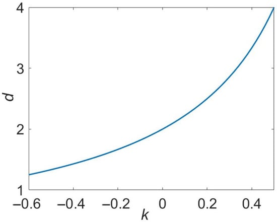
Figure 1. The dependence of $d\left(k\right)$ in accordance with Equation (10).

4. The Parameter k and the Issue of Dimensionality

In the case of $k=-1$, $d=1$ and the corresponding microgeometry can be imagined as a layered periodic system in which the displacement field, magnetic induction, electric or thermal currents, or heat or mass flux are directed normal to the layers. We note that this direction is the only one that is defined in one dimension. As the ratio of the 1D lattice period to a macroscopic length scale (such as the wavelength of light, characteristic scales of potential or temperature variation, or diffusion length) tends to zero, LE is known to be exact.

The case of $k=0$ yields $d=2$ and results in the LLE, Equation (2), which is particularly frequently used to describe various effective physical characteristics of composite media. The main results for 2D systems have been obtained with the use of the Keller-Dykhne duality relation [37,38].

It is well-known that in 2D systems with $f_1=f_2=1/2$, which possess phase-inversion symmetry, the equation

$${\widetilde{ϵ}}_{eff}=\sqrt{{ϵ}_1{ϵ}_2}$$

(11)

holds, independently of the specific microgeometry. It is easy to see that Equation (11) follows from Equation (2) when $f_1=f_2=1/2$. In addition, using Equation (11) one can verify that Equation (2) coincides with the 2D symmetric Bruggeman equation.

What happens if $f_1\ne f_2$? Significant progress in this direction was achieved by Machavariani and Fel [39,40]. They began with the microgeometry of a 2D regular infinite checkerboard and assumed that each square on this checkerboard is itself non-uniform, being composed of smaller (finite) checkerboards. By repeating this recursive procedure indefinitely, Equation (2) can be recovered as the result of an interpolation. However, if the recursion is terminated at a finite stage, Equation (2) becomes approximate. It is important that due to the Keller-Dykhne duality, not only square lattices but also trianglular ones and random spot distributions lead to similar conclusions.

Naturally, the key point is the accuracy of this approximation. To quantify it, Machavariani performed numerical calculations of the effective conductivity for various regular 2D structures [40]. The obtained results show that the discrepancy between the numerically obtained effective conductivity and Equation (2) depends markedly on the phase contrast ${\sigma }_1/{\sigma }_2$, with the deviations remaining small for a low contrast, specifically for $0.2\le {\sigma }_1/{\sigma }_2\le 5$. These findings were shown to hold not only for two-phase composites but also for multi-phase systems.

Another interesting feature of the LLE was noted by Simpkin [3]. He found that under the condition of small Clausius-Mossotti factors,

$$\left|{\displaystyle \frac{{ϵ}_1-{ϵ}_{eff}}{{ϵ}_1+2{ϵ}_{eff}}}\right|\ll 1$$

(12)

and

$$\left|{\displaystyle \frac{{ϵ}_2-{ϵ}_{eff}}{{ϵ}_2+2{ϵ}_{eff}}}\right|\ll 1,$$

(13)

the symmetric 3D Bruggeman equation follows from Equation (2). It is obvious that the conditions (12) and (13) are satisfied under a low contrast assumption, i.e., when $0.5\ll \mid {ϵ}_2/{ϵ}_1\mid \ll 2$.

Of particular interest is the case of $k=1/3$, which corresponds to $d=3$ and yields the LLL equation,

$${ϵ}_{eff}^{1/3}=f_1{ϵ}_1^{1/3}+f_2{ϵ}_2^{1/3}.$$

(14)

This equation was considered in detail by Dube [41] and Banhegui [42]. After analysing experimental data on the effective permittivity of dielectric powders at radio- and micro-wave frequencies, Dube concluded that Equation (14) is accurate (within 3%) up to the dielectric constant about 13, provided that the particle size exceeds 50 μm. At the same time, a comparison of experimental and calculated results for the loss factor shows much larger discrepancy, within 10–20%.

Banhegyi reviewed experimental data on the permittivity of near-spherical dielectric particles dispersed in various liquids for a wide range of filling fractions and pointed out that the LLL equation provides the best fit to experiments (within 1%) compared with several other EMA, except in the case of mineral particles in water. The latter case, however, is characterized by a relatively high dielectric contrast (${ϵ}_1/{ϵ}_2\approx 13.4$), whereas the validity of the LLL equation is presumably limited to the regime $\mid {ϵ}_1-{ϵ}_2\mid \ll {ϵ}_{eff}$, which requires a low (close-to-unity) value of ${ϵ}_1/{ϵ}_2$. Naturally, none of the above mixtures possesses phase-inversion symmetry. Overall, the author concluded that Equation (14) is not applicable to mixtures of nonspherical particles or to systems with high dielectric contrast, especially metal-dielectric composites.

The inconsistency of the LLL equation at high contrast h becomes evident when considering the simplest deterministic geometry possessing phase-inversion symmetry, such as a 3D regular checkerboard. In terms of conductivity, Equation (14) yields ${\sigma }_{eff}/{\sigma }_1\to {\displaystyle \frac{1}{8}}{\sigma }_2/{\sigma }_1$ as ${\sigma }_2\to \infty$, whereas the exact asymptotic result is known to be ${\sigma }_{eff}/{\sigma }_1\to 2\sqrt{{\sigma }_2/{\sigma }_1}$ [43].

Several of recent studies also demonstrate a good predictive capability of the LLL equation, in particular, for such composite systems as iron-based powders [44], fly ash [45], and mixed magnetite-maghemite particle composites [46].

5. Archie’s Law

If $k<1/3$, except for the special cases $k=-1$ and $k=0$, Equation (10) yields non-integer values of d. In addition, if $k>1/3$, then $d>3$. Since such values of d appear non-physical, this issue requires closer examination.

It is well known that for a wide variety of porous rocks with an insulating matrix saturated with a saline (conducting) fluid, the effective conductivity follows so-called Archie’s law [47]

$${\sigma }_{eff}={\sigma }_2{f}_2^m,$$

(15)

where ${\sigma }_2$ and $f_2$ are the conductivity and volume fraction (porosity) of the conducting fluid, respectively. The empirical parameter m is usually referred to as the cementation exponent. It is easy to see that Equation (15) follows directly from Equation (1)—expressed in terms of conductivity—under the high-contrast condition ${\sigma }_1/{\sigma }_2\ll 1$, with $m=1/k$ [18]. Typically, values of $m=1.5-2.5$ ($k=0.4-0.66$) are characteristic of most porous arenaceous sediments, while values of $m=2.5-5$ ($k=0.2-0.4$) occur in some carbonates [47,48].

For our purposes, it is more convenient to consider not Equation (15), but its modified version, which assumes that ${\sigma }_1\ne 0$, so that both phases contribute to the effective conductivity. Modified Archie’s law is given by [49]

$${\sigma }_{eff}={\sigma }_1{(1-f_2)}^p+{\sigma }_2{f}_2^m,$$

(16)

where m and p are empirical constants. Imposing the obvious condition that if ${\sigma }_1={\sigma }_2$, then ${\sigma }_{eff}={\sigma }_1={\sigma }_2$, one has ${(1-f_2)}^p+f_2^m=1$. This, in turn, allows Equation (16) to be rewritten as

$${\sigma }_{eff}/{\sigma }_1=1+f_2^m\left({\displaystyle \frac{{\sigma }_2}{{\sigma }_1}}-1\right).$$

(17)

Comparing this with Equations (3) and (4) yields the only solution for the SDF: $g\left(x\right)=0$ and $C_2=f^{m-1}$. If this case, the second sum rule, Equation (5), breaks down, resulting in a zero first moment. Thus, strictly speaking, Archie’s law is hardly consistent with the BMSR for isotropic media.

At first sight, the above inconsistency may seem surprising and contradictory. In fact, it is important to note that although Equation (15) follows from Equation (1), it is not vice versa. While the condition of topological percolation for both phases is typically satisfied for porous media obeying Archie’s law, the condition of phase-inversion symmetry is generally not met.

In Equation (5), the factor $d^{-1}$ comes from an angular average over the directions of the applied electric field [50]. If microgeometry is anisotropic, the first moment becomes tensorial (it contains a directional dependence). Furthermore, in some cases the spatial dependence d may become ill-defined. For instance, a quasi-2D microstructure is highly nonuniform (structured) within a plane (two directions) and nearly uniform or weakly varying along the third direction; a quasi-3D microstructure (almost isotropic 3D) may be approximately uniform along two directions and slightly non-uniform along the third. Moreover, such phenomenon as 2D-3D (or 3D-2D) crossover can occur [51,52,53,54].

6. The Analysis of Uncertainties

Because the values of the phase conductivities (permittivities) ${\sigma }_i$ (${ϵ}_i$) and their volume fractions $f_i$ are always known with some uncertainty, the measured effective permittivity or conductivity is inherently uncertain. Likewise, an error in the parameter k introduces uncertainty in the calculated effective quantity. The inaccuracy of the effective conductivity $\mathsf{\Delta }{\sigma }_{eff}$ for the LE can be estimated as

$$\mathsf{\Delta }{\sigma }_{eff}={\displaystyle \frac{\partial {\sigma }_{eff}}{\partial k}}\mathsf{\Delta }k+{\displaystyle \frac{\partial {\sigma }_{eff}}{\partial f}}\mathsf{\Delta }f+{\displaystyle \frac{\partial {\sigma }_{eff}}{\partial {\sigma }_2}}\mathsf{\Delta }{\sigma }_2+{\displaystyle \frac{\partial {\sigma }_{eff}}{\partial {\sigma }_1}}\mathsf{\Delta }{\sigma }_1.$$

(18)

Let us now evaluate the partial derivatives $I_1=\partial {\sigma }_{eff}/\partial k$, $I_2=\partial {\sigma }_{eff}/\partial f$ and $I_3=\partial {\sigma }_{eff}/\partial {\sigma }_2$ (the derivative $\partial {\sigma }_{eff}/\partial {\sigma }_1$ can be determined analogously to $I_3$ due to symmetry). After straightforward algebra, one obtains for $k\ne 0$:

$$I_1^{\left(k\right)}={\displaystyle \frac{{\sigma }_{eff}}{k}}\left[{\displaystyle \frac{(1-f){\sigma }_1^k\ln {\sigma }_1+f{\sigma }_2^k\ln {\sigma }_2}{{\sigma }_{eff}^k}}-\ln {\sigma }_{eff}\right],$$

(19)

$$I_2^{\left(k\right)}={\displaystyle \frac{{\sigma }_{eff}^{1-k}}{k}}({\sigma }_2^k-{\sigma }_1^k),$$

(20)

$$I_3^{\left(k\right)}=f{\left({\displaystyle \frac{{\sigma }_{eff}}{{\sigma }_2}}\right)}^{1-k}.$$

(21)

At $k\to 0$, using l’Hôpital’s rule, one has

$$I_1^{\left(0\right)}={\displaystyle \frac{1}{2}}f(1-f){\sigma }_{eff}{\ln }^2({\sigma }_2/{\sigma }_1),$$

(22)

$$I_2^{\left(0\right)}={\sigma }_{eff}\ln ({\sigma }_2/{\sigma }_1),$$

(23)

$$I_3^{\left(0\right)}=f{\sigma }_{eff}/{\sigma }_2.$$

(24)

The values of the parameter k are usually obtained by fitting to experimental data. Since $f_i$ and ${\sigma }_1$ (or ${ϵ}_i$) are known only with some uncertainty, the inaccuracy of the parameter k can be estimated as

$$\mathsf{\Delta }k=I_1^{-1}(\mathsf{\Delta }{\sigma }_{eff}-I_2\mathsf{\Delta }f-I_3\mathsf{\Delta }{\sigma }_2-I_4\mathsf{\Delta }{\sigma }_1).$$

(25)

It is therefore useful to estimate the partial derivative $I_1$.

If we are interested in small $\mathsf{\Delta }k$, large values of the partial derivative $I_1$ are preferable. In the limit of ${\sigma }_2/{\sigma }_1\to 1$, both partial derivatives $I_1^0$ and $I_1^{(1/3)}$ are small and attain their maximum values at $f_2=1/2$. As seen in Figure 2, when the contrast ${\sigma }_2/{\sigma }_1$ increases, the peak of $I_1$ shifts monotonically from lower to higher values of $f_2$. In particular, at ${\sigma }_2/{\sigma }_1=100$, $I_1^{(1/3)}$ reaches its maximum value at $f_2\simeq 0.68$, whereas $I_1^{\left(0\right)}$ reaches its maximum at $f_2\simeq 0.83$. In all cases, the derivative $I_1$ is small either when the contrast h is low (i.e., close to unity) or when $f_2$ is close to 0 or 1. In the limit ${\sigma }_2/{\sigma }_1\to \infty$, the partial derivative $I_1$ reaches its maximum under the condition $\partial I_1/\partial f_2=0$. One can verify that, in this limit, the maximum of $I_1^{\left(0\right)}$ occurs as $f_2\to 1$, while the maximum of $I_1^{(1/3)}$ occurs at $f_2=e^{-1/3}\simeq 0.717$.

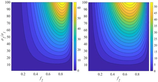
Figure 2. The partial derivatives $I_1^{\left(0\right)}$ (left panel) and $I_1^{(1/3)}$ (right panel).

7. Conclusions

In this paper, we have assessed applicability of widely used general Lichtenecker equation for isotropic composite media. The key findings of our study can be summarized as follows:

(1)

The Lichtenecker equation is compatible with the spectral representation only at $k\to 0$ (logarithmic Lichtenecker equation) in 2D and $k=1/3$ (Landau-Lifshitz-Looyenga equation) in 3D.

(2)

In 3D, the Lichtenecker equation is applicable only for low contrast h, even for composites possessing phase-inversion symmetry.

(3)

Although Archie’s is confirmed in many experiments for porous media, this does not, by itself, validate the Lichtenecker equation.

(4)

If the empirical parameter k of the Lichtenecker equation is determined by fitting to experimental data, small errors in phase volume fractions and/or their conductivities and permittivities can lead to significant inaccuracies in k, especially when $f_2$ is close to 0 or 1, or when the contrast parameter h is low.

In conclusion, great care must be taken when using the Lichtenecker equation, particularly for the effective permittivity or conductivity of metal-dielectric mixtures. Although it sometimes yields reasonable results, in most cases its use is not physically justified.

References

- Lichtenecker, K. Die Dielektrizitätskonstante natürlicher und künstlicher Mischkörper. Phys. Z. 1926, 27, 115–158. [Google Scholar]
- Lichtenecker, K. Der elektrische Leitungswiderstand künstlicher und natürlicher Aggregate. Phys. Z. 1924, 25, 225–233. [Google Scholar]
- Simpkin, R. Derivation of Lichtenecker’s logarithmic mixture formula from Maxwell’s equations. IEEE Trans. Microw. Theory Tech. 2010, 58, 545–550. [Google Scholar] [CrossRef]
- Erle, U.; Regier, M.; Persch, C.; Schubert, H. Dielectric properties of emulsions and suspensions: Mixture equations and measurement comparisons. J. Microw. Power Electromag. Energy 2000, 35, 185–190. [Google Scholar] [CrossRef]
- Yan, Y.; Gonzalez-Cortes, S.; Yao, B.; Slocombe, D.R.; Porch, A.; Cao, F.; Xiao, T.; Edwards, P.P. Rapid, non-invasive characterization of the dispersity of emulsions via microwaves. Chem. Sci. 2018, 9, 6975–6980. [Google Scholar] [CrossRef]
- Robinson, D.A.; Jones, S.B.; Wraith, J.M.; Or, D.; Friedman, S.P. A review of advances in dielectric and electrical conductivity measurement in soils using time domain feflectometry. Vadose Zone J. 2003, 2, 444–475. [Google Scholar] [CrossRef]
- Su, C.; Wu, C.C.; Yang, C. Developing the dielectric mechanisms of polyetherimide/multiwalled carbon nanotube/(Ba0.8Sr0.2)(Ti0.9Zr0.1)O3 composites. Nanoscale Res. Lett. 2012, 7, 132. [Google Scholar] [CrossRef] [PubMed]
- Headland, D.; Thurgood, P.; Stavrevski, D.; Withayachumnankul, W.; Abbott, D.; Bhaskaran, M.; Sriram, S. Doped polymer for low-loss dielectric material in the terahertz range. Opt. Mater. Express 2015, 5, 1373–1380. [Google Scholar] [CrossRef]
- Pérez-Campos, R.; Monzó-Cabrera, J.; Fayos-Fernández, J.; Díaz-Morcillo, A.; Martínez-González, A.; Lozano-Guerrero, A.; Pedreño-Molina, J.; García-Gambín, J. Dielectric characterization of fabric aggregates around the 2.45 GHz ISM band under various humidity, density, and temperature conditions. Materials 2023, 16, 4428. [Google Scholar] [CrossRef] [PubMed]
- Kiley, E.M.; Yakovlev, V.V.; Ishizaki, K.; Vaucher, S. Applicability study of classical and contemporary models for effective complex permittivity of metal powders. J. Microw. Power Electromag. Energy 2012, 46, 26–38. [Google Scholar] [CrossRef]
- Akhtar, M.J.; Tiwari, N.K.; Devi, J.; Mahmoud, M.; Link, G.; Thumm, M. Determination of effective constitutive properties of metal powders at 2.45 GHz for microwave processing applications. Frequenz 2014, 68, 69–81. [Google Scholar] [CrossRef]
- Xiao, X.; Ihamouten, A.; Villain, G.; Dérobert, X. Use of electromagnetic two-layer wave-guided propagation in the GPR frequency range to characterize water transfer in concrete. NDT E Intern. 2017, 86, 164–174. [Google Scholar] [CrossRef]
- Hickson, D.; Boivin, A.; Daly, M.G.; Ghent, R.; Nolan, M.C.; Tait, K.; Cunje, A.; Tsai, C.A. Near surface bulk density estimates of NEAs from radar observations and permittivity measurements of powdered geologic material. Icarus 2018, 306, 16–24. [Google Scholar] [CrossRef]
- Balčiūnas, S.; Ivanov, M.; Banys, J.; Ueno, S.; Wada, S. In search of an artificial morphotropic phase boundary: Lead-free barium titanate based composites. Lith. J. Phys. 2020, 60, 225–234. [Google Scholar] [CrossRef]
- Boughriet, A.; Allahdin, O.; Poumaye, N.; Tricot, G.; Revel, B.; Lesven, L.; Wartel, M. Micro-analytical study of a zeolites/geo-polymers/quartz composite, dielectric behaviour and contribution to Brønsted sites affinity. Ceramics 2022, 5, 908–927. [Google Scholar] [CrossRef]
- Anandakrishnan, S.S.; Nelo, M.; Tabeshfar, M.; Kraft, V.; Khansur, N.H.; Peräntie, J.; Bai, Y. Influence of the permittivity between fillers and binders on the properties of upside-down composites for recycling purposes. Mater. Adv. 2025, 6, 6694–6710. [Google Scholar] [CrossRef]
- de Lima, O.A.L.; Clennell, M.B.; Nery, G.G.; Niwas, S. A volumetric approach for the resistivity response of freshwater shaly sandstones. Geophysics 2005, 70, F1–F10. [Google Scholar] [CrossRef]
- Glover, P. A generalized Archie’s law for n phases. Geophysics 2010, 75, E247–E265. [Google Scholar] [CrossRef]
- Antepara, I.; Fiala, L.; Pavlík, Z.; Černý, R. Moisture dependent thermal properties of hydrophilic mineral wool: Application of the effective media theory. Mater. Sci. (Medžiagotyra) 2015, 21, 449–454. [Google Scholar] [CrossRef]
- Fuchs, S.; Schütz, F.; Förster, H.J.; Förster, A. Evaluation of common mixing models for calculating bulk thermal conductivity of sedimentary rocks: Correction charts and new conversion equations. Geothermics 2013, 47, 40–52. [Google Scholar] [CrossRef]
- Parke, L.; Hooper, I.R.; Hicken, R.J.; Dancer, C.E.J.; Grant, P.S.; Youngs, I.J.; Sambles, J.R.; Hibbins, A.P. Heavily loaded ferrite-polymer composites to produce high refractive index materials at centimetre wavelengths. APL Mater. 2013, 1, 042108. [Google Scholar] [CrossRef]
- Wang, Y.; Edwards, E.; Hooper, I.; Clow, N.; Grant, P.S. Scalable polymer-based ferrite composites with matching permeability and permittivity for high-frequency applications. Appl. Phys. A 2015, 120, 609–614. [Google Scholar] [CrossRef]
- Kočí, V.; Maděra, J.; Krejčí, T.; Kruis, J.; Černý, R. Efficient techniques for solution of complex computational tasks in building physics. Adv. Civil Eng. 2019, 2019, 3529360. [Google Scholar] [CrossRef]
- Guo, R.; Roscow, J.; Bowen, C.; Luo, H.; Huang, Y.; Ma, Y.; Zhou, K.; Zhang, D. Significantly enhanced permittivity and energy density in dielectric composites with aligned BaTiO3 lamellar structures. J. Mater. Chem. A 2020, 8, 3135–3144. [Google Scholar] [CrossRef]
- Schulgasser, K. On a phase interchange relationship for composite materials. J. Math. Phys. 1976, 17, 378–381. [Google Scholar] [CrossRef]
- Stroud, D.; Milton, G.W.; De, B.R. Analytical model for the dielectric response of brine-saturated rocks. Phys. Rev. B 1986, 34, 5145–5153. [Google Scholar] [CrossRef]
- Ghosh, K.; Fuchs, R. Spectral theory for two-component porous media. Phys. Rev. B 1988, 38, 5222–5236. [Google Scholar] [CrossRef] [PubMed]
- Ghosh, K.; Fuchs, R. Critical behavior in the dielectric properties of random self-similar composites. Phys. Rev. B 1991, 44, 7330–7333. [Google Scholar] [CrossRef]
- Tuncer, E. Geometrical description in binary composites and spectral density representation. Materials 2010, 3, 585–613. [Google Scholar] [CrossRef]
- Fuchs, R.; Ghosh, K. Optical and dielectric properties of self-similar structures. Phys. A 1994, 207, 185–196. [Google Scholar] [CrossRef]
- Goncharenko, A.V. Spectral density function approach to homogenization of binary mixtures. Chem. Phys. Lett. 2004, 400, 462–468. [Google Scholar] [CrossRef]
- Tuncer, E.; Bowler, N.; Youngs, I.J. Application of the spectral density function method to a composite system. Phys. B 2006, 373, 306–312. [Google Scholar] [CrossRef]
- Dmitruk, M.; Goncharenko, A.; Venger, E. Optics of Small Particles and Composite Media; Naukova Dumka: Kyiv, Ukraine, 2009. [Google Scholar]
- Goncharenko, A.V.; Lozovski, V.; Venger, E. Lichtenecker’s equation: Applicability and limitations. Opt. Commun. 2000, 174, 19–32. [Google Scholar] [CrossRef]
- Looyenga, H. Dielectric constants of heterogeneous mixtures. Physica 1965, 31, 401–406. [Google Scholar] [CrossRef]
- Landau, L.; Lifshitz, E. Electrodynamics of Continuous Media; Pergamon Press: Oxford, UK; New York, NY, USA; Beijing, China; Frankfurt, Germany, 1984. [Google Scholar]
- Keller, J.B. The theorem on the conductivity of a composite medium. J. Mathem. Phys. 1964, 5, 548–549. [Google Scholar] [CrossRef]
- Dykhne, A.M. Conductivity of a two-dimensional two-phase system. Sov. Phys. JETP 1971, 32, 63–65, Translation of Zh. Eksp. Teor. Fiz. 1970, 59, 110–115. [Google Scholar]
- Machavariani, V.S.; Voronel, A. Estimation of the intrinsic heterogeneity of ionic glass-forming melts. Phys. Rev. E 2000, 61, 2121–2124. [Google Scholar] [CrossRef] [PubMed]
- Machavariani, V.S. Universality in effective conductivity of regular 2D and 3D composites. J. Phys. Condens. Matter 2001, 13, 6797–6812. [Google Scholar] [CrossRef]
- Dube, D. Study of Landau-Lifshitz-Looyenga’s formula for dielectric correlation between powder and bulk. J. Phys. D Appl. Phys. 1970, 3, 1648–1652. [Google Scholar] [CrossRef]
- Bánhegyi, G. Comparison of electrical mixture rules for composites. Colloid Polym. Sci. 1986, 264, 1030–1050. [Google Scholar] [CrossRef]
- Soderberg, M.; Grimvall, G. Current distributions for a two-phase material with chequer-board geometry. J. Phys. Solid State Phys. 1983, 16, 1085. [Google Scholar] [CrossRef][Green Version]
- Yang, R.B.; Hsu, S.D.; Lin, C.K. Frequency-dependent complex permittivity and permeability of iron-based powders in 2–18 GHz. J. Appl. Phys. 2009, 105, 07A527. [Google Scholar] [CrossRef]
- Sreenivas, V.N.; Karthik, D.; Kumar, V.A. Determination of complex permittivity of fly ash for potential electronic applications. Appl. Mech. Mater. 2012, 110–116, 4292–4296. [Google Scholar] [CrossRef]
- Sainz-Menchón, M.; González de Arrieta, I.; Echániz, T.; Nader, K.; Insausti, M.; Canizarès, A.; Rozenbaum, O.; López, G. Quantifying lattice vibrational modes and optical conductivity in mixed magnetite–maghemite nanoparticles. Phys. Chem. Chem. Phys. 2025, 27, 8498–8509. [Google Scholar] [CrossRef]
- Cai, J.; Wei, W.; Hu, X.; Wood, D.A. Electrical conductivity models in saturated porous media: A review. Earth Sci. Rev. 2017, 171, 419–433. [Google Scholar] [CrossRef]
- Glover, P. What is the cementation exponent? A new interpretation. Lead. Edge 2009, 28, 82–85. [Google Scholar] [CrossRef]
- Glover, P.W.; Hole, M.J.; Pous, J. A modified Archie’s law for two conducting phases. Earth Planet. Sci. Lett. 2000, 180, 369–383. [Google Scholar] [CrossRef]
- Kantor, Y.; Bergman, D. Improved rigorous bounds on the effective elastic moduli of a composite material. J. Mech. Phys. Solids 1984, 32, 41–62. [Google Scholar] [CrossRef]
- Gelb, L.D.; Gubbins, K.E.; Radhakrishnan, R.; Sliwinska-Bartkowiak, M. Phase separation in confined systems. Rep. Prog. Phys. 1999, 62, 1573. [Google Scholar] [CrossRef]
- Dvoynenko, M.M.; Goncharenko, A.V.; Venger, E.F.; Pinchuk, A.O. Effects of dimension on optical transmittance of semicontinuous gold films. Phys. B 2001, 299, 88–93. [Google Scholar] [CrossRef]
- Mokhtari, M.; Zekri, L.; Kaiss, A.; Zekri, N. Effect of film thickness on the width of percolation threshold in metal-dielectric composites. Condens. Matter Phys. 2016, 19, 43001. [Google Scholar] [CrossRef]
- Chalyi, A.V. Effective fractal dimension at 2d-3d crossover. Fract. Fract. 2022, 6, 739. [Google Scholar] [CrossRef]
Disclaimer/Publisher’s Note: The statements, opinions and data contained in all publications are solely those of the individual author(s) and contributor(s) and not of MDPI and/or the editor(s). MDPI and/or the editor(s) disclaim responsibility for any injury to people or property resulting from any ideas, methods, instructions or products referred to in the content. |
© 2025 by the authors. Licensee MDPI, Basel, Switzerland. This article is an open access article distributed under the terms and conditions of the Creative Commons Attribution (CC BY) license (https://creativecommons.org/licenses/by/4.0/).