Three-Dimensional Surface High-Precision Modeling and Loss Mechanism Analysis of Motor Efficiency Map Based on Driving Cycles

Abstract

Amid fossil-fuel depletion and worsening environmental impacts, battery electric vehicles (BEVs) are pivotal to the energy transition. Energy management in BEVs relies on accurate motor efficiency maps, yet real-time onboard control demands models that balance fidelity with computational cost. To address map inaccuracy under real driving and the high runtime cost of 2-D interpolation, we propose a driving-cycle-aware, physically interpretable quadratic polynomial-surface framework. We extract priority operating regions on the speed–torque plane from typical driving cycles and model electrical power $P_e$ as a function of motor speed $n$ and mechanical power $P_m$. A nested model family (M3–M6) and three fitting strategies—global, local, and region-weighted—are assessed using $R^2$, RMSE, a computational complexity index (CCI), and an Integrated Criterion for accuracy–complexity and stability (ICS). Simulations on the Worldwide Harmonized Light Vehicles Test Cycle, the China Light-Duty Vehicle Test Cycle, and the Urban Dynamometer Driving Schedule show that region-weighted fitting consistently achieves the best or near-best ICS; relative to Global fitting, mean ICS decreases by 49.0%, 46.4%, and 90.6%, with the smallest variance. Regarding model order, the four-term M4 $\left(+P_m^2\right)$ offers the best accuracy–complexity trade-off. Finally, the region-weighted fitting M4 $\left(+P_m^2\right)$ polynomial model was integrated into the vehicle-level economic speed planning model based on the dynamic programming algorithm. In simulations covering a 27 km driving distance, this model reduced computational time by approximately 87% compared to a linear interpolation method based on a two-dimensional lookup table, while achieving an energy consumption deviation of about 0.01% relative to the lookup table approach. Results demonstrate that the proposed model significantly alleviates computational burden while maintaining high energy consumption prediction accuracy, thereby providing robust support for real-time in-vehicle applications in whole-vehicle energy management.

1. Introduction

As global energy demand continues to climb and environmental pollution worsens, the energy crisis and climate change have become major challenges facing the world [1,2]. Massive carbon dioxide emissions, excessive reliance on fossil fuels, and the resulting depletion of resources not only exacerbate the instability of energy supply but also inflict significant negative impacts on the ecological environment [3]. Therefore, promoting energy transition, reducing greenhouse gas emissions, and vigorously developing renewable energy have become urgent requirements for achieving sustainable development [4,5].

To address these challenges, the automotive industry is progressively transitioning toward energy efficiency and low-carbon transformation. New energy vehicles (NEVs)—especially pure electric vehicles (PEVs)—are central to this transition [6]. Compared with conventional fuel-powered vehicles, PEVs offer significant advantages such as zero pollution and zero emissions in their powertrain systems. However, to fully leverage these benefits in real-world transportation, precise and real-time energy management strategies must be implemented in the controllers. The motor efficiency map serves as the core of energy management control strategies based on dynamic programming (DP) [7].

In many studies, motor efficiency maps underpin design [8,9], control [10,11], and planning [12,13]. Adeleke et al. [14] used maps to formulate a torque-distribution strategy for four-in-wheel-motor EVs under a joint objective of optimal torque split and energy efficiency. Liang et al. [15] built a two-layer linear time-varying model predictive control (LTV-MPC) torque-vectoring framework grounded in maps, achieving co-optimization of energy saving and yaw-stability in simulation and hardware-in-the-loop (HIL) tests. Ju et al. [16] leveraged maps in a model predictive control (MPC)-based speed-planning scheme to enable real-time eco-cruising for connected hybrid electric vehicles (HEVs). Du et al. [17] proposed a real-time predictive energy-management strategy that combines speed prediction with map-based optimization. These examples illustrate that the fidelity and usability of efficiency maps directly condition the performance of energy management and component co-design.

However, conventional motor efficiency maps [18,19,20] are typically obtained from dynamometer bench tests at discrete operating points. Due to limitations in sensor placement and experimental costs, these data often exhibit high sparsity, noise interference, and uneven distribution. Directly employing two-dimensional interpolation and lookup table (LUT) methods in energy management strategies [18] presents two major challenges: On one hand, in data-sparse regions and boundary areas, external interpolation instability and noise amplification effects can introduce significant errors [19]; On the other hand, for global optimization algorithms like DP that require frequent access to efficiency data, repeated interpolation incurs substantial computational and temporal overhead, severely compromising the algorithm’s real-time performance and limiting deployment on in-vehicle controllers.

Consequently, recent research has increasingly adopted fitting methods to replace linear interpolation. For example, Jun et al. [20] combined finite-element analysis with neural networks to rapidly construct efficiency maps for permanent-magnet synchronous motors, significantly reducing computational time. Cheng et al. [21] proposed surface fitting of efficiency maps together with FE-based interpolation to evaluate cycle efficiency quickly. Abhay et al. [22] extracted loss coefficients from efficiency maps using particle-swarm optimization coupled with a physics-based loss model, enabling deeper insight into loss sources without additional computational burden. Mısır et al. [23] developed a machine learning-based multivariate polynomial regression estimation model to estimate motor efficiency and iron core loss profiles, thereby overcoming these costly processes in finite element analysis. In addition, other established fitting approaches have been used, including low-order polynomial regression [24], Gaussian process regression (GPR) [25], piecewise polynomials [26], linear regression [27], and nonlinear least-squares (NLS) fitting [28].

Although machine learning (ML) [29] and Kriging methods may achieve low fitting errors and offer good flexibility under sufficient data conditions, they still exhibit the following limitations in the vehicle energy management and optimal speed planning scenarios addressed in this paper: First, in terms of computational complexity and real-time performance during operation, ML models typically involve extensive parameter computations, making it difficult to meet the computational cost requirements for high-frequency model invocations demanded by algorithms like DP. Secondly, these methods inherently constitute black-box models whose parameters lack clear physical interpretation, hindering mechanism analysis. Furthermore, machine learning approaches typically require large-scale training data to avoid overfitting, whereas the motor efficiency map data obtained from bench tests is limited in scale, rendering their generalization capabilities disadvantageous in this scenario. More importantly, existing approaches largely overlook the distribution characteristics of real-world driving cycles. They often prioritize global fitting accuracy while neglecting the distribution patterns of actual high-frequency operating regions. This results in insufficient fitting precision and weak generalization capabilities within practical operating ranges, thereby compromising engineering applicability. In contrast, the polynomial model structure adopted in this paper is simple with fewer parameters. It achieves stable, high-precision, and highly generalizable fitting based solely on bench test datasets. Therefore, establishing a computationally efficient, physically interpretable motor efficiency model [30,31,32] that aligns with real-world operating conditions holds significant theoretical research value and engineering importance.

To address these issues, this paper proposes a high-precision modeling framework for motor efficiency maps [33] oriented to typical driving cycles (e.g., WLTC, CLTC, UDDS) or commonly used operating conditions. The framework aims to balance model accuracy, computational efficiency, and consistency with physical loss mechanisms. Its core idea is to incorporate region awareness and low-term, interpretable polynomials. The decision-making process proposed in this paper consists of six steps, as shown in Figure 1. First, various input data are collected, including vehicle parameters, motor efficiency maps, and driving conditions. The second step involves mapping the speed curve of the driving cycle to motor operating points $\left(n_{moto{r}_{rpm}},T_{motor}\right)$ based on the vehicle’s longitudinal dynamics. Using the driving conditions and vehicle parameters, the preferred operating region $R$ is selected from the axially aligned rectangular envelope. The third step converts all valid points from $\left(n_{moto{r}_{rpm}},T_{motor}\right)$ to $\left(n_{moto{r}_{rpm}},P_m,P_e\right)$ within the motor efficiency map. Using $\left(n_{moto{r}_{rpm}},P_m\right)$ as input, a quadratic polynomial surface model for $P_e$ is established. This model selection stems from two key considerations: First, the clear physical relationship between electrical and mechanical power facilitates unification across diverse operating modes. Second, quadratic polynomials can simultaneously represent linear trends and coupled relationships with minimal parameters, balancing computational cost while maintaining model accuracy. The fourth step involves three fitting strategies—global fitting, regional fitting, and region-weighted fitting—combined with four configurations (M3–M6) to form 24 distinct configurations, each undergoing regression fitting to enhance model accuracy in high-priority regions while maintaining reasonable global predictions. This step is completed offline, eliminating additional in-vehicle computational load. Step 5: For all configurations, calculate the global and regional coefficient of determination ($R^2$) and the root-mean-square error (RMSE) metrics. Combine these with the computational complexity indicator (CCI) to construct the integrated criterion for accuracy, complexity and stability (ICS). The final deployable model is selected based on the minimum ICS value to achieve a balance between accuracy and complexity. In this study, the region-weighted fitting configuration M4 (+$P_m^2$) consistently achieved optimal or near-optimal results across multiple iterations. Step 6: To validate the accuracy and computational complexity of the proposed model, it was integrated into a vehicle-wide economic speed planning algorithm based on dynamic programming, replacing the high-frequency calls of the traditional LUT-2D interpolation approach. Results demonstrate that the proposed method significantly reduces computational load while maintaining energy consumption prediction accuracy, thereby providing engineering value for real-time in-vehicle applications of high-frequency optimization algorithms like DP.

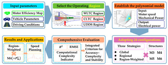
Figure 1. High-precision 3D surface modeling of motor efficiency maps for driving cycles and model selection decision flowchart.

In summary, the main contributions are as follows:

(1)

A driving-cycle–oriented, region-aware 3-D modeling strategy is proposed. Using the 2-D distribution of speed–torque, a working region $R$ is delineated, prioritizing prediction accuracy and robustness within cycle-relevant operating areas.

(2)

A nested family of quadratic models (M3–M6) is constructed, and the optimal order is selected under a balanced consideration of regional accuracy, global robustness, and computational complexity.

(3)

Explicit correspondences are established between polynomial terms and physical loss mechanisms (e.g., copper and iron losses), ensuring interpretability and providing a basis for engineering diagnosis.

(4)

To validate the engineering applicability of this polynomial model in vehicle energy management, this paper applies it to dynamic programming-based vehicle economic speed planning, enabling offline decision-making and online invocation. The region-weighted M4 $\left(+P_m^2\right)$ model is selected and embedded into the economic speed planning framework, using a low-cost polynomial to replace the traditional two-dimensional LUT method for obtaining motor efficiency. In simulation tests of the economic speed planning, computational time was reduced by 87% compared to the LUT method. Simultaneously, the deviation in energy consumption prediction results relative to the LUT method was only 0.01%. Simulation results demonstrate that, on one hand, this model significantly reduces computational burden; on the other hand, the energy consumption results corresponding to the planned speeds maintain high prediction accuracy. This provides excellent engineering benefits for real-time onboard energy management applications and online economic speed planning.

The organizational structure of this paper is described as follows. Section 2 details the theoretical foundations and the driving-cycle-based modeling method. Section 3 presents the evaluation framework and fitting results. In Section 4, to validate the practical applicability of the proposed fitting strategies, this paper applies polynomial fitting models based on different strategies to vehicle speed planning for fuel efficiency. It systematically evaluates their performance in energy management and further discusses the suitable scenarios for different fitting strategies. Section 5 concludes the paper and outlines future research directions.

2. Theoretical Basis and Modeling Foundation

To enhance model accuracy and practicality, this section develops a mapping from standardized driving-cycle speed profiles to operating points on the motor efficiency map $(n_{\mathrm{motor}},T_{\mathrm{motor}})$ using longitudinal vehicle dynamics, thereby identifying priority high-efficiency operating regions for model training. On this basis, we further formalize the physical relationships among mechanical power $P_m$, electrical power $P_e$, and efficiency $\eta$, and propose a physically interpretable quadratic polynomial surface that models $P_e$ as a function of motor speed and mechanical power $P_m$. The resulting representation provides a computationally efficient, physically informed description of motor electrical power for use in energy-management optimization.

Before modeling, we first clarify the fundamental assumptions regarding the control strategy. The motor efficiency map based on bench testing in this paper was collected under a fixed and calibrated underlying control strategy. This strategy encompasses key control parameters such as the current regulation loop, modulation scheme, modulation index, and switching frequency. This implies that the efficiency or input/output power data measured at each operating point equivalently incorporates all losses generated under this control strategy. Therefore, the model presented here characterizes the “averaged” total losses—including fundamental and specific harmonic losses—under this calibrated control strategy. It should be noted that variations in harmonic losses resulting from changes in the pulse-width modulation (PWM) strategy, while keeping rotational speed n and mechanical power $P_m$ constant are not explicitly reflected in this model.

2.1. Vehicle Dynamics and Operating Point Extraction

This paper takes a mid-size pure electric vehicle as its research subject. The vehicle-related parameters are listed in Table 1.

Table 1. Main Parameters of Electric Vehicle.

Type	Parameter (Symbol [Unit])	Value
Vehicle	$\mathrm{Mass}m$ [kg]	2100
	$\mathrm{Effective}\mathrm{rolling}\mathrm{radius}r$ [m]	0.359
	$\mathrm{Rolling}\mathrm{resistance}\mathrm{coefficient}{c}_r$ [-]	0.0056
	$\mathrm{Aerodynamic}\mathrm{drag}\mathrm{coefficient}{C}_d$ [-]	0.27
	$\mathrm{Frontal}\mathrm{area}A$ [m2]	2.686
	$\mathrm{Driving}\mathrm{Efficiency}{\eta }_{drive}$ [-]	0.9702
	$\mathrm{Regenerative}-\mathrm{braking}\mathrm{efficiency}{\eta }_{regen}$ [-]	0.9702
Motor	$\mathrm{Rated}\mathrm{Voltage}{U}_{rated}$ [V]	580
	$\mathrm{Maximum}\mathrm{speed}{n}_{max}$ [rpm]	18,000
	$\mathrm{Rated}\mathrm{power}{P}_{e,\mathrm{r}ated}$ [kW]	110
	$\mathrm{Rated}\mathrm{torque}{T}_{rated}$ [Nm]	210
	$\mathrm{Peak}\mathrm{power}{P}_{e,max}$ [kW]	218
	$\mathrm{Peak}\mathrm{torque}{T}_{max}$ [Nm]	440
Battery	SOC [%]	$\left[\mathrm{3,100}\right]$
	$\mathrm{Maximum}\mathrm{charge}/\mathrm{discharge}\mathrm{power}{P}_{bat,\mathrm{m}ax}$ [kW]	215
Reducer	$\mathrm{Final}\mathrm{drive}\mathrm{ratio}{i}_0$ [-]	9.597

To map a driving-cycle speed profile to operating points on the motor torque–speed plane $\left(n_{moto{r}_{rpm}},T_{motor}\right)$, this study first establishes a longitudinal vehicle dynamics model. By Newton’s second law, the required longitudinal tractive force $F_{total}$ is the sum of the inertial term $F_{acc}$, rolling resistance $F_{roll}$, aerodynamic drag $F_{aero}$, and grade force $F_{grade}$:

$$\left\{\begin{array}{l}\begin{array}{l}\begin{array}{l}{F}_{total}=F_{acc}+F_{roll}+F_{aero}+F_{grade}\\ \begin{array}{l}{F}_{acc}=m·a\left(t\right)\\ F_{roll}=mg{c}_r·cos\theta \end{array}\end{array}\\ F_{aero}={\displaystyle \frac{1}{2}}\rho C_{d}A{v}_{mps}^2\left(t\right)\end{array}\\ F_{grade}=mgsin\theta \end{array}\right.,$$

(1)

$$a\left(t\right)={\displaystyle \frac{v_{mps}\left(t+1\right)-v_{mps}\left(t\right)}{dt}},$$

(2)

where $v_{mps}\left(t\right)$ is vehicle speed [$\mathrm{m}/\mathrm{s}$], $a\left(t\right)$ is longitudinal acceleration [$\mathrm{m}/{\mathrm{s}}^2$], $t$ is time [$\mathrm{s}$], $g$ is gravitational acceleration [$\mathrm{m}/{\mathrm{s}}^2],$ $\theta$ is road-grade angle [rad], $\rho$ is air density [$\mathrm{k}\mathrm{g}/{\mathrm{m}}^3$].

The total tractive force is converted to wheel-side torque through the effective wheel radius $r$:

$$T_{\mathrm{w}\mathrm{h}\mathrm{e}\mathrm{e}\mathrm{l}}=F_{\mathrm{t}\mathrm{o}\mathrm{t}\mathrm{a}\mathrm{l}}·r.$$

(3)

With the sign convention $F_{\mathrm{t}\mathrm{o}\mathrm{t}\mathrm{a}\mathrm{l}}>0$ for traction demand and $F_{\mathrm{t}\mathrm{o}\mathrm{t}\mathrm{a}\mathrm{l}}<0$ for braking demand, negative wheel torque can be recuperated through the drivetrain. The wheel angular speed obtained from vehicle speed is:

$${\omega }_{\mathrm{w}\mathrm{h}\mathrm{e}\mathrm{e}\mathrm{l}}\left(t\right)={\displaystyle \frac{v_{\mathrm{m}\mathrm{p}\mathrm{s}}\left(t\right)}{r}}.$$

(4)

Through the overall gear ratio $i_{\mathrm{t}\mathrm{o}\mathrm{t}\mathrm{a}\mathrm{l}}=i_0$, the motor angular speed is ${\omega }_{\mathrm{m}\mathrm{o}\mathrm{t}\mathrm{o}\mathrm{r}}\left(t\right)={\omega }_{\mathrm{w}\mathrm{h}\mathrm{e}\mathrm{e}\mathrm{l}}\left(t\right)i_{\mathrm{t}\mathrm{o}\mathrm{t}\mathrm{a}\mathrm{l}},$ and the motor speed in rpm becomes:

$$n_{moto{r}_{rpm}}(t)={\displaystyle \frac{60}{2\pi }}{\omega }_{\mathrm{m}\mathrm{o}\mathrm{t}\mathrm{o}\mathrm{r}}(t)={\displaystyle \frac{60}{2\pi }}{\displaystyle \frac{v_{\mathrm{m}\mathrm{p}\mathrm{s}}\left(t\right)}{r}}{i}_{\mathrm{t}\mathrm{o}\mathrm{t}\mathrm{a}\mathrm{l}}.$$

(5)

The corresponding motor torque is:

$$T_{\mathrm{m}\mathrm{o}\mathrm{t}\mathrm{o}\mathrm{r}}=\left\{\begin{array}{ll}{\displaystyle \frac{T_{\mathrm{w}\mathrm{h}\mathrm{e}\mathrm{e}\mathrm{l}}}{i_0{\eta }_{\mathrm{d}\mathrm{r}\mathrm{i}\mathrm{v}\mathrm{e}}}}& ,T_{\mathrm{w}\mathrm{h}\mathrm{e}\mathrm{e}\mathrm{l}}\ge 0\left(\mathrm{traction}\right),\hfill \\ {\displaystyle \frac{T_{\mathrm{w}\mathrm{h}\mathrm{e}\mathrm{e}\mathrm{l}}}{i_0}}·{\eta }_{\mathrm{r}\mathrm{e}\mathrm{g}\mathrm{e}\mathrm{n}}& ,T_{\mathrm{w}\mathrm{h}\mathrm{e}\mathrm{e}\mathrm{l}}<0\left(\mathrm{regeneration}\right).\hfill \end{array}\right.$$

(6)

This treatment yields a unified expression for motor torque across both traction and regenerative-braking modes, subject to the physical limits of the machine and battery: $0\le n_{moto{r}_{rpm}}\le n_{max}$, $\left|T_{motor}\right|\le T_{max}$, $\left|P_e\right|\le P_{e,max}$, together with SOC and power constraints.

After obtaining $\left(n_{\mathrm{m}\mathrm{o}\mathrm{t}\mathrm{o}\mathrm{r},\mathrm{r}\mathrm{p}\mathrm{m}},T_{\mathrm{m}\mathrm{o}\mathrm{t}\mathrm{o}\mathrm{r}}\right)$ from the driving cycle, this study employs an interval-envelope method to emphasize high-utilization and critical operating conditions. Specifically, an axis-aligned operating domain is constructed by imposing lower and upper bounds on speed and torque, thereby defining a high-efficiency priority region for fitting while remaining consistent with engineering practice and avoiding uncertainties from complex statistical assumptions. The envelope is

$$R=[n_{\mathrm{m}\mathrm{i}\mathrm{n}},n_{\mathrm{m}\mathrm{a}\mathrm{x}}]\times [T_{\mathrm{m}\mathrm{i}\mathrm{n}},T_{\mathrm{m}\mathrm{a}\mathrm{x}}].$$

(7)

To illustrate how different cycles shape the operating region, we visualize the resulting point clouds for WLTC, UDDS, and CLTC (Figure 2). WLTC covers a broader span in the medium-to-high speed range and forms distinct high-torque bands during multiple accelerations; UDDS concentrates on low-to-medium speeds with frequent stop-and-go and a high share of regenerative events; CLTC lies in between, combining medium-speed cruising with several accelerations. The sizes of $R$ differ markedly across the three cycles, reflecting their distinct speed/acceleration structures and providing an objective basis for parameterizing the subsequent Local and region-weighted fitting schemes.

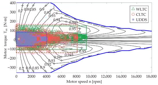
Figure 2. Operating-point clouds for WLTC/UDDS/CLTC on the motor torque–speed plane.

It is worth emphasizing that, in this study, the sign of the motor torque $T_{\mathrm{m}\mathrm{o}\mathrm{t}\mathrm{o}\mathrm{r}}$ is used to distinguish operating quadrants. A single coordinate system $\left(n_{moto{r}_{rpm}},T_{\mathrm{m}\mathrm{o}\mathrm{t}\mathrm{o}\mathrm{r}}\right)$ therefore describes both traction $(T_{\mathrm{m}\mathrm{o}\mathrm{t}\mathrm{o}\mathrm{r}}\ge 0)$ and regenerative braking $(T_{\mathrm{m}\mathrm{o}\mathrm{t}\mathrm{o}\mathrm{r}}<0)$ without domain switching or mode-specific LUT. Moreover, when constructing models that use $P_m={\displaystyle \frac{n_{moto{r}_{rpm}}{T}_{motor}}{9.55}}[W]$ as an input, the sign of $T_{\mathrm{m}\mathrm{o}\mathrm{t}\mathrm{o}\mathrm{r}}$ naturally propagates to $P_m$, enabling both quadrants to be represented within the same function family for electrical power. Compared with efficiency-map table lookup, this unified treatment mitigates numerical jitter and interpolation error near state transitions.

2.2. Modeling an Interpretable Motor Electrical Power Function

To replace two-dimensional motor efficiency maps based on LUT interpolation, this paper establishes a quadratic polynomial model with motor electrical power $P_e$ as the output, using motor speed $n_{moto{r}_{rpm}}$ and mechanical power $P_m$ as the independent variables. The model unifies the drive and brake quadrants, uses a compact set of terms, and provides clear correspondence to the primary loss mechanisms. It is consistent with energy conservation and canonical loss physics, while offering closed-form evaluation and parameter interpretability, which facilitates replacing traditional look-up tables in high-frequency energy-management algorithms such as dynamic programming.

Although the operational state of an electric motor is fundamentally determined by both rotational speed ($n_{moto{r}_{rpm}}$) and torque ($T_{motor}$), we adopt mechanical power ($P_m$) to reparameterize the speed-torque plane. This choice does not alter the fundamental physics. Within the motor’s operational range, a one-to-one correspondence exists between ($n_{moto{r}_{rpm}}$, $T_{motor}$) and ($n_{moto{r}_{rpm}}$, $P_m$). However, it significantly improves the regularity of the surface to be fitted. In the ($n_{moto{r}_{rpm}}$, $T_{motor}$) coordinate system, the efficiency map $\eta \left(n_{moto{r}_{rpm}},T_{motor}\right)$ exhibits pronounced nonlinearity and a multi-peak/multi-trough structure. This makes it challenging for low-order polynomials to achieve high-precision global fitting, particularly near operating condition transitions such as traction and regenerative braking, where significant errors can occur. In contrast, when motor speed and mechanical power are used as independent variables and motor electrical power as the dependent variable, the resulting three-dimensional surface becomes smoother and more regular. Its advantage lies in the fact that mechanical power itself is the product of speed and torque. Under constant torque conditions, $P_m$ exhibits a linear relationship with speed. Intuitively, in the ($n_{moto{r}_{rpm}}$, $P_m$) space, using $P_m$ as the dependent variable yields a “mechanical power plane.” Our target dependent variable is the motor’s electrical power. This means that, building upon the original linear relationship, we overlay a relatively smooth modulation function determined by efficiency characteristics, thereby upgrading this plane into an “electrical power surface.” This permits accurate approximation using a low-order polynomial, achieving an optimal balance between physical fidelity and model simplicity for controller implementation.

The proposed model unifies the drive and brake quadrants, employs a compact set of terms, and provides clear correspondence to primary loss mechanisms. It remains consistent with energy conservation and canonical loss physics while offering the practical advantages of closed-form evaluation and parameter interpretability. These features facilitate the replacement of traditional LUTs in high-frequency energy-management algorithms such as dynamic programming.

The following conventions are adopted: motor speed $n_{moto{r}_{rpm}}$ is expressed in $rpm$; motor torque $T_{motor}$ in $Nm$. Taking the battery terminal as the reference, the electrical power $P_e$ is defined as the forward power from the battery to the motor:

$$P_e=\left\{\begin{array}{cc}{\displaystyle \frac{P_m}{\eta \left(n,T_{motor}\right)}},\hfill & \hfill \mathrm{t}\mathrm{r}\mathrm{a}\mathrm{c}\mathrm{t}\mathrm{i}\mathrm{o}\mathrm{n},\\ P_m·\eta \left(n,T_{motor}\right),\hfill & \hfill \mathrm{r}\mathrm{e}\mathrm{g}\mathrm{e}\mathrm{n}\mathrm{e}\mathrm{r}\mathrm{a}\mathrm{t}\mathrm{i}\mathrm{o}\mathrm{n},\end{array}0<\right.\eta \le 1.$$

(8)

Simultaneously, the above relation implies $\mathrm{s}\mathrm{i}\mathrm{g}\mathrm{n}\left(P_e\right)=\mathrm{s}\mathrm{i}\mathrm{g}\mathrm{n}\left(P_m\right)$. Leveraging this property, the set $(n_{moto{r}_{rpm}},P_m)$ can be treated as unified independent variables across operating quadrants, thereby avoiding numerical discontinuities induced by cross-quadrant piecewise fitting and boundary stitching. Furthermore, from energy conservation,

$$P_e=P_m+P_{loss}\left(n,T_{motor}\right),$$

(9)

where the total loss $P_{\mathrm{loss}}$ includes iron loss, eddy-current loss, hysteresis loss, copper loss, bearing friction loss and stray loss. These mechanisms can be approximated by low-order polynomials in the $(n_{moto{r}_{rpm}},P_m)$ domain, yielding an electric-power model that is both sufficiently accurate and minimally complex.

Given the nonlinear dependence of total losses on speed and load, we adopt the following six quadratic basis functions:

$$\varphi =\left\{P_m^2,n_{moto{r}_{rpm}}·P_m,P_m,n_{moto{r}_{rpm}}^2,n_{moto{r}_{rpm}},1\right\}.$$

(10)

The physical interpretability of this model stems from the term–mechanism mapping. Crucially, the preceding choice of $P_m$ over $T_{\mathrm{motor}}$ as a regressor is not merely for unifying quadrant representation. While it achieves that, its primary merit is mathematical: the coordinate transformation from $(n_{\mathrm{motor}},T_{\mathrm{motor}})$ to $(n_{\mathrm{motor}},P_m)$ yields a far more regular and smooth response surface for $P_e$, which is inherently amenable to low-order polynomial approximation. This transforms a problem of fitting a complex, multi-modal efficiency map into one of modulating a near-linear baseline, thereby enabling both high accuracy and simplicity.

(1)

${a_{1}P}_m^2$ is the leading term associated with armature copper loss. Neglecting changes in magnetic flux and field-weakening effects, the stator current $I$ is approximately proportional to the electromagnetic torque. Accordingly, the copper loss can equivalently be modeled as a quadratic function of the load:

$$P_{Cu}={\displaystyle \frac{m_1{\int }_{t_0}^{t_0+T}{I}^2\left(t\right)R\mathrm{d}t}{T}}$$

(11)

where $m_1$ is the number of motor phases, $T$ is the repetition period of the current waveform, $R$ is the winding resistance, $t$ is the time variable of integration, $t_0$ is an arbitrary initial time marking the start of the averaging window, and $I\left(t\right)$ is the current waveform. Therefore, the use of $P_m$ integrates the coupling effect between rotational speed and torque into a mathematically convenient single variable without compromising physical generality. This provides a compact and easily fitted model form for the primary loss mechanism.

(2)

$a_2{n}_{moto{r}_{rpm}}·P_m$ denotes the load-related additional electromagnetic loss term. This term accounts for additional electromagnetic losses induced by the load current, including air-gap field distortion, eddy currents in the end-winding and slot regions, and tooth-harmonic effects; its magnitude increases with both rotational speed and load.

(3)

$a_3{P}_m$ is a low-order purely linear term used to absorb components in the low-frequency region that are not fully captured by the quadratic term, as well as approximately linear contributions, such as inverter conduction loss. It also compensates, to some extent, for minor system errors near the boundaries of the efficiency map, improving the fit to baseline data over the operating domain.

(4)

$a_4{n}_{moto{r}_{rpm}}^2$ and $a_5{n}_{moto{r}_{rpm}}$ are the dominant terms for frequency-dependent losses. Hysteresis loss and eddy-current loss exhibit an approximately linear–quadratic mixed dependence. The hysteresis component can be written as

$$P_{\mathrm{H}\mathrm{y}}=C_{\mathrm{H}\mathrm{y}}{B}_m^{n}fV,$$

(12)

which scales with the area of the hysteresis loop (determined by the peak flux density $B_m$), the excitation frequency $f$, and the volume $V$ of the ferromagnetic material. Here $P_{\mathrm{H}\mathrm{y}}$ denotes the hysteresis loss, $C_{\mathrm{H}\mathrm{y}}$ is a material-dependent hysteresis coefficient, and $n$ typically lies in the range $1.5~2$; for estimation, $n=2$ is commonly adopted.

An alternating magnetic field induces closed-loop currents in the core, i.e., eddy currents, which generate heat and thus eddy-current loss. This loss can be expressed as

$$P_{Ft}=C_{Ft}{B}_m^2{f}^2{d}^{2}V,$$

(13)

where $P_{Ft}$ denotes the eddy-current loss, $C_{Ft}$ is a material-dependent eddy-loss coefficient, and $d$ is the core lamination thickness. Because the excitation frequency f is proportional to the rotational speed, the eddy-current loss is proportional to $n_{moto{r}_{rpm}}^2$.

During rotor motion, friction between the rotor and the surrounding air produces windage loss, which depends on the rotor surface roughness, roundness, and rotational speed.

(5)

$a_6$ is a static-loss term that represents machine-specific constant losses and modeling bias. A large $\left|a_6\right|$ suggests checking the normalization of quantities, the extrapolation near the boundaries of the efficiency map, and the quality of zero-load data.

In this mapping, the even term $P_m^2$ captures the symmetric load effect across quadrants, whereas the odd term $n_{moto{r}_{rpm}}·P_m$ accounts for the asymmetric electric-power behavior between driving and braking at the same speed. Consequently, the six-term model captures the dominant trends governed by symmetric mechanisms while representing modest asymmetries with few degrees of freedom, thereby striking a balance between interpretability and expressive power.

2.3. Three Fitting Strategies Across Operating Regions

To replace the traditional efficiency map look-up in the DP with a low-computation-cost, interpretable, two-quadrant-unified alternative, this section builds on Section 2.1, which extracts operating points from the driving cycle, and Section 2.2, which specifies the physical variables and functional forms, and proposes three fitting strategies: global fitting, regional fitting, and region-weighted fitting. All three approaches are based on the same six-term quadratic polynomial model. They differ only in how the available samples are selected and weighted, and thus target, respectively: robustness across the entire domain, high local accuracy in a priority region, and a balanced trade-off between regional accuracy and global robustness.

Crucially, the data used for fitting in this paper comprises all valid operating points from the motor efficiency LUT. Each valid efficiency value measured on the $(n_{\mathrm{motor}},T_{\mathrm{motor}})$ plane during bench testing is converted into a data sample in the form $(n_{\mathrm{motor}},P_m,P_e)$. Traditional LUT methods also rely on this efficiency map, storing discrete efficiency values in the $(n_{\mathrm{motor}},T_{\mathrm{motor}})$ plane and performing two-dimensional interpolation during runtime. Thus, in terms of data origin, the quadratic polynomial model proposed in this paper and the LUT method are both based entirely on a single set of test data. The fundamental difference lies in replacing the “LUT + interpolation” data operation with a compact closed-form functional relationship. The training dataset comprises 1458 discrete $(n_{\mathrm{motor}},T_{\mathrm{motor}})$ points defined in the original efficiency MAP—exactly matching the data used by traditional interpolation methods and requiring no sampling during fitting—covering 27 speed points (discrete intervals of 1000 $\mathrm{r}\mathrm{p}\mathrm{m})$ and 54 torque points (from −360 $\mathrm{N}\mathrm{m}$ to 400 $\mathrm{N}\mathrm{m}),$ thus fully encompassing both traction and regenerative braking quadrants. The core requirement for training data is that samples must adequately represent the entire operating range, encompassing the full spectrum of speed and torque.

Based on the axis-aligned rectangular envelope $R=\left[n_{min},n_{max}\right]\times \left[T_{min},T_{max}\right]$ defined in Section 2.1 and the model inputs $(n_{\mathrm{m}\mathrm{o}\mathrm{t}\mathrm{o}\mathrm{r},\mathrm{r}\mathrm{p}\mathrm{m}},P_m)$, we compute the equivalent torque ${\widehat{T}}_i={\displaystyle \frac{P_{m,i}}{n_i}}·9.55$ to determine whether the operating point lies within $R$, thereby identifying the priority region as shown in Figure 3. The priority operating regions R is obtained through the process of “driving cycle—work point cloud—axis-aligned bounding rectangle,” representing the sub-area that actually operates at high frequency in the energy management strategy.

$$insideIdx:(n_{min}\le n_i\le n_{max})\cap (T_{min}\le {\widehat{T}}_i\le T_{max}).$$

(14)

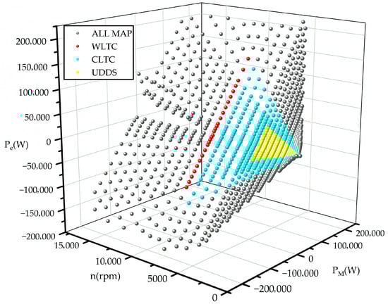
Figure 3. Map with inside regions—WLTC/CLTC/UDDS.

For notational convenience, we construct the design matrix $X$ with rows $\left[P_{m,i}^2,n·P_{m,i},P_{m,i},n_i^2,n_i,1\right],$ and the observation vector $y=[P_{e,1},\dots ,P_{e,N}{]}^{\mathrm{\top }}$. The parameter vector $a=[a_1,\dots ,a_6{]}^{\mathrm{\top }}$ is estimated so that $Xa$ closely approximates $y$. To avoid ill-conditioning, all three strategies adopt a very small ridge regularization $\lambda ={10}^{-8}$, which improves numerical stability without altering the physical interpretation.

2.3.1. Global Fitting Strategy

Global fitting uses all valid samples in the operating domain and seeks to minimize the overall error. This strategy distributes the model degrees of freedom uniformly over the $\left(n_{moto{r}_{rpm}},P_m\right)$ plane and exhibits good extrapolation robustness and boundary smoothness. Its computational cost is markedly lower than the frequent quadratic interpolations required by the DP algorithm. However, under practical operating conditions it may fail to guarantee the desired accuracy within commonly used subregions. Therefore, the global fit is not always optimal. The estimator is

$$\widehat{a}=\arg \underset{a}{\min }{‖Xa-y‖}_2^2+\lambda {‖a‖}_2^2.$$

(15)

2.3.2. Region-Weighted Fitting Strategy

To prioritize accuracy in frequently used operating regions while preserving global reasonableness, we construct a region-weighted fitting method under the same model by introducing a sample-weight matrix $W=diag\left(w_i\right)$:

$$w_i=\left\{\begin{array}{cc}{w}_{in}\ge 1\hfill & \hfill ,\left(n_i,T_i\right)\in R,\\ 1,\hfill & \hfill otherwise,\end{array}\right.$$

(16)

$$\widehat{a}=\arg \underset{a}{\min }{\left(Xa-y\right)}^{\mathrm{T}}W\left(Xa-y\right)+\lambda {‖a‖}_2^2.$$

(17)

Unlike global fitting and the approach that fits only inside the priority region, the region-weighted fitting balances boundary continuity and extrapolation stability while reflecting realistic operating conditions. By tuning the in-region weight $w_{in}$, a compromise point is selected on a validation set such that the regional error is reduced and the global error changes only slightly. This method is well suited when a specific operating condition, driving cycle, or historical data are available, delivering high accuracy in the priority region without sacrificing global behavior.

2.3.3. Regional Fitting

For regional fitting restricted to the priority operating region, all model degrees of freedom are devoted to the in-region domain. However, because the optimization completely ignores samples outside the priority region, the extrapolation capability is weak. When the motor operating points imposed by a given driving cycle are strictly confined to $R$, such as in urban driving cycles or fixed-condition tests, the most direct approach is to construct the model using only samples within $R$:

$$\widehat{a}=\arg \underset{a}{\min }{‖X_{R}a-y_R‖}_2^2+\lambda {‖a‖}_2^2,\left(n_i,T_i\right)\in R$$

(18)

To further reduce computational cost, we decrease the number of polynomial terms, thereby markedly lowering the total floating-point operations and cumulative latency. To ensure accuracy under practical operating conditions, under all three strategies (global fitting, regional fitting, and region-weighted fitting), we progressively truncate higher-order terms and solve models with 3–6 terms (M3–M6). Model selection is then performed using a composite metric that jointly considers accuracy, stability, and computational complexity. This replaces the traditional table lookup and interpolation, enabling stable and efficient computation in full-vehicle simulations and in the controller.

3. Comprehensive Evaluation and Fitting Results

3.1. Evaluation Indicators

To comprehensively assess the polynomial efficiency-map model across different driving cycles and fitting strategies, we adopt a set of evaluation indicators along three dimensions—accuracy, stability, and complexity. The indicators include the coefficient of determination ($R^2$), the root-mean-square error (RMSE), and a computational complexity indicator (CCI). For model comparison and selection, we also report an integrated criterion for accuracy–complexity and stability (ICS) that balances these three aspects.

1.

$R^2$.

Used to compare the measured electric-power vector $y=\{P_{e,i}{\}}_{i=1}^N$ with the model prediction $\widehat{y}=\{{\widehat{P}}_{e,i}{\}}_{i=1}^N$:

$$R^2=1-{\displaystyle \frac{\sum _{i=1}^N{\left(P_{e,i}-{\widehat{P}}_{e,i}\right)}^2}{\sum _{i=1}^N{\left(P_{e,i}-{\overline{P}}_{e,i}\right)}^2}},R^2\in [\mathrm{0,1}].$$

(19)

Here, ${\overline{P}}_e$ is the sample mean of the observations. $R^2$ values closer to 1 indicate a better fit and a higher proportion of the variance in $P_e$ explained by the model. Because this study spans both traction and braking quadrants, $R^2$ provides a primary domain-wide consistency indicator.

2.

RMSE.

RMSE is a common indicator for quantifying the discrepancy between model predictions and measured values. It is computed as the square root of the mean squared prediction error:

$$\mathrm{R}\mathrm{M}\mathrm{S}\mathrm{E}=\sqrt{{\displaystyle \frac{1}{N}}{\sum }_{i=1}^N{\left(P_{e,i}-{\widehat{P}}_{e,i}\right)}^2}.$$

(20)

A smaller RMSE indicates smaller prediction error and thus higher predictive accuracy. In this work, the absolute error is measured in watts, which makes comparisons across strategies more intuitive. We report both the global RMSE and the in-region RMSE to diagnose model effectiveness in the key operating domain.

3.

CCI.

To maintain accuracy while minimizing computational cost, we introduce a computational complexity index as a reference indicator:

$$\mathrm{C}\mathrm{C}\mathrm{I}=N_{mul}+c_{add}{N}_{add}=\left(k+d\right)+c_{add}\left(k-1\right),k\in \left\{\mathrm{3,4},\mathrm{5,6}\right\},d\in \left\{\mathrm{0,1},\mathrm{2,3}\right\}$$

(21)

Here, $N_{\mathrm{mul}}$ is the number of multiplications required to evaluate a $k$-term model, and $N_{\mathrm{add}}$ is the number of additions needed to accumulate the $k$ terms. Each term requires one coefficient–feature multiplication, hence $k$ multiplications. If the selected feature set contains any of $\left\{P_m^2,n_{moto{r}_{rpm}}·P_m,n_{moto{r}_{rpm}}^2\right\}$, each such feature needs one extra multiplication to form the feature itself, contributing $d$ additional multiplications. Therefore $N_{\mathrm{mul}}=k+d$. Summing the $k$ terms require $k-1$ additions, i.e., $N_{\mathrm{add}}=k-1$. Because additions are typically cheaper than multiplications on embedded controllers, we weight them by $c_{\mathrm{add}}\in \left[\mathrm{0,1}\right]$ and set $c_{\mathrm{add}}=0.5$ in our experiments. A smaller CCI indicates lower unit-cost computational complexity. Table 2 summarizes CCI under typical settings.

Table 2. CCI for different polynomial orders.

Mk	Polynomial Structures	CCI
M3	$\left\{P_m,n_{moto{r}_{rpm}},1\right\}$	4.0
M4 $\left(+P_m^2\right)$	$\left\{P_m^2,P_m,n_{moto{r}_{rpm}},1\right\}$	6.5
M4 $\left(+n_{moto{r}_{rpm}}^2\right)$	$\left\{P_m,n_{moto{r}_{rpm}}^2,n_{moto{r}_{rpm}},1\right\}$	6.5
M4 $\left(+n_{moto{r}_{rpm}}·P_m\right)$	$\left\{P_m,{n_{moto{r}_{rpm}}·P_m,n}_{moto{r}_{rpm}},1\right\}$	6.5
M5 $\left(-n_{moto{r}_{rpm}}·P_m\right)$	$\left\{P_m^2,P_m,n_{moto{r}_{rpm}}^2,n_{moto{r}_{rpm}},1\right\}$	9.0
M5 $\left(-n_{moto{r}_{rpm}}^2\right)$	$\left\{P_m^2,n_{moto{r}_{rpm}}·P_m,P_m,n_{moto{r}_{rpm}},1\right\}$	9.0
M5 $\left(-P_m^2\right)$	$\left\{n_{moto{r}_{rpm}}·P_m,P_m,n_{moto{r}_{rpm}}^2,n_{moto{r}_{rpm}},1\right\}$	9.0
M6	$\left\{P_m^2,n_{moto{r}_{rpm}}·P_m,P_m,n_{moto{r}_{rpm}}^2,n_{moto{r}_{rpm}},1\right\}$	11.5

4.

ICS.

To prioritize accuracy in the priority region while retaining global usability and real-time performance, we define a dimensionless integrated criterion for accuracy–complexity and stability to rank polynomial structures (M3–M6) and fitting strategies. Let ${\sigma }_{P_e}$ denote the standard deviation of the electric-power samples on the given driving cycle. The dynamic range $\mathrm{m}\mathrm{a}\mathrm{x}\left(P_e\right)-\mathrm{m}\mathrm{i}\mathrm{n}\left(P_e\right)$ may be used instead for scale normalization. Using the in-region indicators $(R_R^2,{\mathrm{R}\mathrm{M}\mathrm{S}\mathrm{E}}_{\mathrm{R}})$ and the global indicators $(R_G^2,{\mathrm{R}\mathrm{M}\mathrm{S}\mathrm{E}}_{\mathrm{G}})$, and measuring complexity by CCI normalized by ${\mathrm{C}\mathrm{C}\mathrm{I}}_{\mathrm{M}6}$, the ICS is defined as

$$\mathrm{I}\mathrm{C}\mathrm{S}=\alpha \left[\beta \left(1-R_R^2\right)+\left(1-\beta \right){\displaystyle \frac{{\mathrm{R}\mathrm{M}\mathrm{S}\mathrm{E}}_{\mathrm{R}}}{{\sigma }_{P_e}}}\right]+\left(1-\alpha \right)\left[\beta \left(1-R_G^2\right)+\left(1-\beta \right){\displaystyle \frac{{\mathrm{R}\mathrm{M}\mathrm{S}\mathrm{E}}_{\mathrm{G}}}{{\sigma }_{P_e}}}\right]+\gamma {\displaystyle \frac{\mathrm{C}\mathrm{C}\mathrm{I}}{\mathrm{C}\mathrm{C}{\mathrm{I}}_{{\mathrm{M}}_6}}}$$

(22)

To ensure an optimal balance between accuracy in priority regions, global robustness, and computational complexity, this paper proposes a comprehensive evaluation metric for selecting interpretable mechanism models tailored for in-vehicle deployment. In algorithms like DP that frequently invoke motor efficiency maps, replacing traditional LUT-based two-dimensional interpolation with closed-form polynomials necessitates balancing model accuracy with computational overhead. ICS comprehensively considers three factors: regional accuracy, global robustness, and computational complexity. It introduces accuracy metrics within the priority working region $R$ and on globally effective samples to avoid optimizing only local regions, which could degrade extrapolation performance. The RMSE is normalized by ${\mathsf{\sigma }}_{{\mathrm{P}}_{\mathrm{e}}}$ to eliminate dimensional effects and ensure comparability across different datasets. Computational cost is measured by the computational complexity index (CCI) and normalized using ${\mathrm{CCI}}_{\mathrm{M}6}$.

First, $\alpha$ represents the regional accuracy weight. $\alpha =1$ indicates full reliance on regional accuracy, suitable for scenarios with fixed and known operating conditions typical of driving cycles; $\alpha =0$ indicates consideration only of global accuracy, suitable for scenarios with variable or wide-ranging operating conditions where regional fitting accuracy is not required. For unknown operating conditions approximately describable by typical cycles, $\alpha \in [0.7,0.9]$ is adopted in this paper. The intermediate value $\alpha =0.8$ is used as the default, where the optimal model configuration remains unchanged within this range. $\beta$ balances trend-fitting goodness-of-fit and root-mean-square normalized prediction error, with a default of 0.5. Lower $\beta$ emphasizes absolute error, while higher $\beta$ prioritizes the overall trend. $\gamma$ is a complexity penalty coefficient reflecting in-vehicle ECU computational constraints. This paper sets $\gamma =0.002$ based on the order-of-magnitude matching principle: Since $\left(1−R^2\right)$ and ${\displaystyle \frac{{\mathrm{R}\mathrm{M}\mathrm{S}\mathrm{E}}_{\mathrm{G}}}{{\sigma }_{P_e}}}$ typically have an order of magnitude of ${10}^{-2}$, while $\mathrm{C}\mathrm{C}{\mathrm{I}}_{{\mathrm{M}}_6}$ is $O\left(1\right)$, setting $\gamma$ to ${10}^{-3}$ to achieve lightweight suppression without significant accuracy improvement, while maintaining the “accuracy-driven” model selection principle. In practical deployment, $\gamma$ can be adjusted inversely based on runtime constraints until the selected model simultaneously meets real-time and accuracy requirements. Thus, holding all else fixed, any improvement in any component decreases ICS, ensuring comparability and stable model selection. Table A1, Table A2 and Table A3 (WLTC, CLTC, and UDDS, respectively) summarize the M$k$ configurations under the three fitting strategies, reporting $R_R^2$, $R_G^2$, ${\mathrm{R}\mathrm{M}\mathrm{S}\mathrm{E}}_{\mathrm{R}}$, and ${\mathrm{R}\mathrm{M}\mathrm{S}\mathrm{E}}_{\mathrm{G}}$ in Appendix A.

3.2. Analysis of Fitting Results

Under the ICS defined in Section 3.1 ($\alpha =0.8$, $\beta =0.5$, $\gamma =0.002$), we evaluate three driving cycles across three strategies and four polynomial structures (M3–M6), yielding 24 configurations in total. The results show that region-weighted fitting attains the best or near-best ICS on all three cycles. Across structures, the four-term model M4 that includes $P_m^2$ generally offers a more favorable accuracy–complexity trade-off, although the optimal order and the best strategy vary slightly with the distribution of operating points.

3.2.1. WLTC Results

Figure 4 illustrates the ICS comparison across polynomial structures (M3–M6) and fitting strategies under WLTC, showing that M4 $\left(+P_m^2\right)$ with region-weighted fitting achieves the best overall trade-off. For WLTC, the average ICS over the three strategies is ordered as region-weighted fitting < regional fitting < global fitting. Relative to global fitting, the region-weighted average is reduced by 49.0%. Relative to regional fitting, it is further reduced by 1.76%. This indicates that, for WLTC, starting from the low-order M3 structure, introducing a single quadratic term $P_m^2$ already captures the power-dominated quadratic losses.

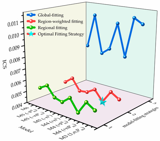
Figure 4. ICS comparison across model configurations—WLTC.

From the perspective of the global optimum, M4 $\left(+P_m^2\right)$ with region-weighted fitting yields the smallest ICS, followed closely by M4 $\left(+P_m^2\right)$ with regional fitting, with a gap of only 0.29%. Using the best ICS within each structure as the baseline, the best M3 is 13.5% worse than the best M4 $\left(+P_m^2\right)$, while increasing the order to the best M6 is 18.5% worse than the best M4 $\left(+P_m^2\right)$. These structure-level comparisons clearly reveal the benefit of region awareness: under the same weighting setup, the error reduction from increasing model order does not offset the penalty from added complexity.

Meanwhile, the contrast among fitting strategies is pronounced across operating regions. For example, with M4 $\left(+n_{moto{r}_{rpm}}·P_m\right)$, region-weighted fitting improves ICS over global fitting by 55.4%; with M3, the improvement is 57.6%. The absolute gains are on the order of ${10}^{-3}$.

Overall, the preferred configuration is M4 $\left(+P_m^2\right)$ with region-weighted fitting, which achieves the best balance among the three objectives—in-region accuracy, global robustness, and computational complexity. Under tighter compute budgets, M3 with region-weighted fitting can serve as a low-complexity alternative. Under the current weighting, increasing the order to M5/M6 is not recommended: the error reduction from higher-order terms is insufficient to offset the CCI penalty, and the ICS consequently increases.

3.2.2. CLTC Results

Figure 5 shows the ICS profiles of the three fitting strategies across polynomial structures (M3–M6) under CLTC, indicating that region-weighted fitting, especially the M4 $\left(+P_m^2\right)$ configuration, delivers the most favorable accuracy–complexity–stability trade-off. The ranking of the fitting strategies is consistent with WLTC results: region-weighted < regional < global. Relative to global and regional fitting, the mean ICS of region-weighted fitting is reduced by 46.4% and 2.6%, respectively. The global optimum is M4 $\left(+P_m^2\right)$ with region-weighted fitting, followed closely by M4 $\left(+P_m^2\right)$ with regional fitting, with a gap of $1.84\times {10}^{-5}$. These strategy-level comparisons highlight the benefit of region awareness: for example, with the M3 structure, region-weighted fitting lowers ICS by 54.0% compared with global fitting. Under the CLTC speed distribution, switching the strategy to region-weighted yields much larger gains than fine structural adjustments among higher-order terms; further increasing the order causes the complexity penalty to dominate, and the ICS rises.

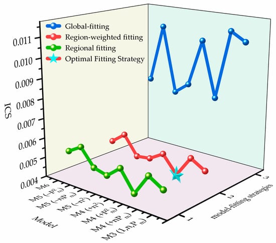
Figure 5. ICS comparison across model configurations—CLTC.

Compared with M3–region-weighted fitting under the same strategy, M4 $\left(+P_m^2\right)$–region-Weighted fitting reduces ICS by 13.0%. By contrast, further increasing the order yields diminishing returns: the ICS of M6 with region-weighted fitting is 18.2% higher than the best configuration, while M4 $\left(+n_{moto{r}_{rpm}}^2\right)$–region-weighted and M4 $\left(+n_{moto{r}_{rpm}}·P_m\right)$–region-weighted fitting are 20.6% and 25.2% worse, respectively. These results indicate that, under the CLTC speed distribution, adding $P_m^2$ to the minimal three-term baseline (M3) markedly improves the fit without materially increasing CCI.

In the M5 configuration, the region-weighted form M5 $\left(-n_{moto{r}_{rpm}}·P_m\right)$ attains the best ICS, followed by M5 ($-n_{moto{r}_{rpm}}^2$) with region-weighted fitting, while M5 $\left(-P_m^2\right)$ with region-weighted fitting performs the worst. This further indicates that the $P_m^2$ term offers the highest benefit–cost ratio in medium- and low-order models. The result is consistent with a “power-dominated” loss mechanism: when the number of terms is limited, prioritizing $P_m^2$ delivers the largest error reduction without materially increasing CCI.

In summary, under CLTC, the preferred solution is the same as under WLTC: M4 $\left(+P_m^2\right)$ with region-weighted fitting, which achieves the best balance among the three objectives: in-region accuracy, global robustness, and computational complexity.

3.2.3. UDDS Results

The UDDS cycle is characterized by low speeds and frequent stop-and-go events, unlike cycles with a higher share of high-speed operation. Under this cycle, global fitting exhibits pronounced distortion. The ordering of ICS across strategies is region-weighted fitting < regional fitting < global fitting. Relative to global fitting, region-weighted fitting reduces the mean ICS by 90.6%. Relative to regional fitting, it further reduces ICS by 40.8%.

Figure 6 contrasts the ICS across polynomial structures (M3–M6) and fitting strategies under UDDS, from which region-weighted fitting—most notably the M4 $\left(+P_m^2\right)$ configuration—consistently attains the lowest ICS, yielding the best accuracy–complexity–stability balance. The experiments indicate that, while preserving global consistency and boundary continuity, assigning higher weights to the priority region yields substantial ICS reductions on UDDS. Notably, the dispersion differs markedly across strategies: the standard deviation of ICS is $5.84\times {10}^{-4}$ for region-weighted fitting, compared with $3.52\times {10}^{-3}$ for regional fitting and $1.46\times {10}^{-2}$ for global fitting. These results underscore the necessity of region awareness and weighting for short-trip, stop-and-go cycles such as UDDS.

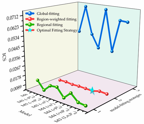
Figure 6. ICS comparison across model configurations—UDDS.

From a global-optimum standpoint, M4 $\left(+P_m^2\right)$ with region-weighted fitting attains the smallest ICS, followed by M5 $\left(-n_{moto{r}_{rpm}}·P_m\right)$ with region-weighted fitting, and then M4 $\left(+n_{moto{r}_{rpm}}^2\right)$ with region-weighted fitting. Even the best regional fitting model, M3–regional, yields an ICS of 0.004776, which is 6.25% higher than the optimum. Under the highly skewed speed distribution of UDDS, adding the $P_m^2$ term to the minimal three-term baseline (M3) markedly improves overall accuracy and stability, and it offers a better error–complexity trade-off than simply raising the order to M5/M6. Meanwhile, relative to regional fitting, region-weighted fitting maintains comparable in-region accuracy while substantially reducing extrapolation sensitivity and the contribution of small errors, thereby retaining a consistent advantage in ICS.

Within the M$k$ structure, M4 $\left(+P_m^2\right)$ outperforms the same-order alternatives M4 $\left(+n_{moto{r}_{rpm}}^2\right)$ and M4 $\left(+n_{moto{r}_{rpm}}·P_m\right)$. Under the best strategy (region-weighted fitting), the ICS of M4 $\left(+n_{moto{r}_{rpm}}^2\right)$ is 5.24% higher than that of M4 $\left(+P_m^2\right)$, and the best five-term option M5 $\left(-n_{moto{r}_{rpm}}·P_m\right)$ still exceeds M4 $\left(+P_m^2\right)$. This is consistent with a power-dominated loss mechanism: under the low-speed, light-load, stop-and-go conditions of UDDS, allocating one term to $P_m^2$ is the most effective use of limited degrees of freedom, whereas adding $n_{moto{r}_{rpm}}^2$ or the interaction $n_{moto{r}_{rpm}}·P_m$ alone provides too little marginal error reduction to offset the complexity penalty, causing ICS to rise.

It is worth noting that although M3–regional ranks near the top, it still lags M4 $\left(+P_m^2\right)$–region-weighted by a clear margin and is more prone to degradation when extrapolating to uncovered boundaries or atypical operating points, so it is not general enough for engineering use. For the M$k$ structure under UDDS, regional and region-weighted produce similar ICS. When the operation is strictly confined to the priority region, regional fitting may serve as an engineering fallback, but its boundary continuity and extrapolation stability are inferior to region-weighted fitting, and its overall ranking remains lower.

In summary, the recommended option is M4 $\left(+P_m^2\right)$ with region-weighted fitting. This combination achieves the best trade-off among the three objectives—in-region accuracy, global robustness, and computational complexity—and it dominates in both the mean and the variance of ICS. When computation is tight, M3–region-weighted fitting can be used as a backup. Moving to higher orders (M5/M6) is not advised unless the reductions in both in-region and global errors clearly offset the added complexity penalty. Overall, M4 $\left(+P_m^2\right)$–region-weighted shows the strongest suitability and robustness for UDDS. It can replace table lookup with a lightweight online implementation and meets the real-time and extrapolation-safety requirements of stop-and-go urban cycles.

With the weights used in this paper, the three cycles lead to a consistent conclusion: region-weighted fitting provides a better compromise among the three objectives and can serve as the default strategy. For the M$k$ structure, all cycles select M4 $\left(+P_m^2\right)$–region-weighted as the preferred fitting strategy. If compute and memory are ample, the order may be increased while keeping the region and strategy unchanged to further improve target accuracy. Overall, M4 $\left(+P_m^2\right)$–region-weighted fitting is optimal or near-optimal under WLTC, CLTC, and UDDS, demonstrating good robustness under the chosen weights $\alpha =0.8$, $\beta =0.5$, and $\gamma =0.002$.

4. Discussion

This paper proposes a region-aware, interpretable, low-order polynomial framework for high-accuracy motor efficiency maps tailored to typical driving cycles. Using the integrated indicator ICS (composed of $R^2$, RMSE, and CCI), we systematically evaluate three fitting strategies—global fitting, regional fitting, and region-weighted fitting—across four nested polynomial structures (M3–M6). For WLTC, CLTC, and UDDS, the priority operating region is identified from the $(n,T_{\mathrm{motor}})$ distribution. Within this region, ICS is lower than the baseline obtained with global fitting only.

At the application level, this study integrates the fitting strategy framework into a DP-based vehicle-level economic speed planning model. Selecting an urban traffic scenario, the UDDS operating point distribution is adopted as the priority operating zone $R$. Both the traditional LUT-binary interpolation method and the proposed closed-form polynomial model are employed to solve the economic speed trajectory for this urban condition within the same DP framework. To ensure fair comparison, the planned speeds from both methods were input into the same vehicle energy consumption model to calculate power consumption. Using the LUT approach’s energy consumption as a reference, the energy consumption deviation caused by different modeling strategies was statistically analyzed.

Under urban conditions, the energy consumption deviation of the 24 strategies compared to the LUT-based method is shown in Figure 7. Results indicate that global fitting exhibits the highest overall error, while region-weighted fitting and fitting solely within regions yield overall errors acceptable for practical engineering applications. Thus, the priority operating regions selected in this study are effective. When sufficient historical vehicle data exists, the priority operating region can be identified based on its empirical distribution and modeled accordingly, enabling regionalized fitting aligned with actual usage patterns. During global fitting, the broad coverage of motor efficiency maps leads to insufficient accuracy under known urban conditions. To enhance fitting precision in real-world scenarios, we recommend prioritizing historical data or multiple driving cycle condition sets to determine samples in engineering practice. This region R should cover a sufficiently large number of operating points. Additionally, we recommend defaulting to a region-weighted fitting strategy. Switch to global fitting when operating conditions are unknown or span a wide range to ensure usability and extrapolation stability across the entire domain. When operating conditions are defined or historical data exists, defaulting to a regional fitting strategy is advised.

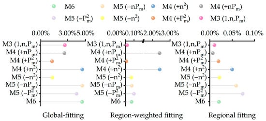
Figure 7. Energy consumption deviation relative to the LUT method benchmark under different strategies.

In terms of computational cost, the LUT-based two-dimensional interpolation method utilizing the motor efficiency map for whole-vehicle economic speed planning requires approximately 4.92 s in simulations covering a driving distance of 27 km. The computational time for economic speed planning using the polynomial model proposed in this paper is shown in Figure 8. The results indicate that embedding the proposed M4 architecture into the vehicle-level economic speed planning reduces computation time to 0.61 s, representing a significant improvement of 87.47%. Therefore, compared to the LUT-based method, the region-weighted fitting strategy of the M4 $\left(+P_m^2\right)$ configuration achieves a substantial reduction in computation time while maintaining an accuracy error of only 0.01%, significantly outperforming other polynomial models.

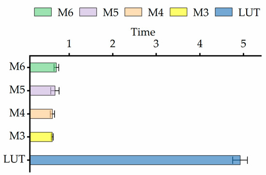
Figure 8. Time required for planning the most economical vehicle speed under different strategies.

The essence of the closed-form polynomial method described herein lies in offline calibration and online low-cost evaluation. When applied to applications requiring frequent calls, such as DP, it replaces LUT interpolation with closed-form functions. Consequently, it can be extended to other components of BEVs. Taking inverters as an example, if inverter efficiency is plotted against speed and torque with efficiency as the coordinate, the modeling framework described herein can be applied. This approach must satisfy physical constraints, such as non-negative losses, to replace LUT interpolation.

5. Conclusions

This paper proposes a quadratic, physically interpretable polynomial model for driving-cycle–oriented motor efficiency maps. By establishing a closed-form map $\left(n_{moto{r}_{rpm}},P_m\right)\to P_e$, the model unifies the traction and regenerative-braking quadrants. Focusing on three strategies—Global fitting, Local fitting, and region-weighted fitting—we evaluate performance under a joint accuracy–stability–computational-complexity framework using $R^2$, RMSE, CCI, and ICS. The simulative results of vehicle-level economic speed planning based on DP demonstrate that this method offers advantages such as computational efficiency, smooth numerical values across all operating conditions, and a favorable balance between accuracy and complexity. It exhibits significant engineering practicality and is suitable for in-vehicle deployment scenarios with high real-time requirements.

Based on real driving cycles, the priority operating region is extracted from the $(n,T_{\mathrm{motor}})$ distribution, and a nested quadratic polynomial family is built. The correspondence between polynomial terms and loss mechanisms is explicitly defined. Across the 24 configurations spanning three cycles and four polynomial structures (M3–M6), the region-weighted fitting strategy consistently achieves the best or near-best ICS performance.

For model selection, the four-term structure M4 $\left(+P_m^2\right)$ strikes the best balance between accuracy and complexity. Adding only $P_m^2$ to the minimal set M3 provides the largest error reduction per unit compute, whereas moving to M5/M6 brings limited gains that usually do not offset the increase in CCI. The modeling and selection process proposed in this paper is universally applicable: for any motor, by sequentially performing region extraction, multi-strategy fitting, and ICS comprehensive evaluation screening based on the motor efficiency chart, vehicle parameters, and operating condition data, one can obtain the optimal fitting strategy and model structure tailored to both the motor and the actual application scenario.

In the planning of vehicle-wide economic speeds, the M4 $\left(+P_m^2\right)$ model with region-weighted fitting replaces the traditional two-dimensional LUT for the motor efficiency map. Results demonstrate that this model reduces computation time by approximately 87% while controlling energy consumption prediction errors within 0.01%, providing an efficient and precise solution for real-time onboard energy management. Based on the above research, future work will proceed in three directions: First, introduce joint modeling of temperature/weak magnetic fields with inverters and batteries to enhance fitting accuracy under high-speed, strong transient, and low SOC conditions. Secondly, for in-vehicle deployment, ECU/HIL/real-vehicle validation will be conducted. The proposed method model will be embedded into the controller to leverage dynamic real-world data for recalibration and robustness enhancement. This will further enable closed-loop benefits through collaborative design with the controller. Third, incorporate control parameters such as modulation index and switching frequency into the model as input variables in compact form to distinguish harmonic loss differences under various control strategies, thereby constructing a universal motor loss model suitable for control co-optimization.

References

- Li, Z.Z.; Su, C.-W.; Moldovan, N.-C.; Umar, M. Energy Consumption within Policy Uncertainty: Considering the Climate and Economic Factors. Renew. Energy 2023, 208, 567–576. [Google Scholar] [CrossRef]
- Hussain, S.A.; Razi, F.; Hewage, K.; Sadiq, R. The Perspective of Energy Poverty and 1st Energy Crisis of Green Transition. Energy 2023, 275, 127487. [Google Scholar] [CrossRef]
- Ahmad, M.; Zheng, J. Do Innovation in Environmental-Related Technologies Cyclically and Asymmetrically Affect Environmental Sustainability in BRICS Nations? Technol. Soc. 2021, 67, 101746. [Google Scholar] [CrossRef]
- Sorlei, I.-S.; Bizon, N.; Thounthong, P.; Varlam, M.; Carcadea, E.; Culcer, M.; Iliescu, M.; Raceanu, M. Fuel Cell Electric Vehicles—A Brief Review of Current Topologies and Energy Management Strategies. Energies 2021, 14, 252. [Google Scholar] [CrossRef]
- Ren, L.; Zhou, S.; Ou, X. Life-Cycle Energy Consumption and Greenhouse-Gas Emissions of Hydrogen Supply Chains for Fuel-Cell Vehicles in China. Energy 2020, 209, 118482. [Google Scholar] [CrossRef]
- Jiang, F.; Yuan, X.; Hu, L.; Xie, G.; Zhang, Z.; Li, X.; Hu, J.; Wang, C.; Wang, H. A Comprehensive Review of Energy Storage Technology Development and Application for Pure Electric Vehicles. J. Energy Storage 2024, 86, 111159. [Google Scholar] [CrossRef]
- Xu, N.; Kong, Y.; Yan, J.; Zhang, Y.; Sui, Y.; Ju, H.; Liu, H.; Xu, Z. Global Optimization Energy Management for Multi-Energy Source Vehicles Based on “Information Layer—Physical Layer—Energy Layer—Dynamic Programming” (IPE-DP). Appl. Energy 2022, 312, 118668. [Google Scholar] [CrossRef]
- Eckert, J.J.; Silva, F.L.; Da Silva, S.F.; Bueno, A.V.; De Oliveira, M.L.M.; Silva, L.C.A. Optimal Design and Power Management Control of Hybrid Biofuel–Electric Powertrain. Appl. Energy 2022, 325, 119903. [Google Scholar] [CrossRef]
- Krüger, B.; Keinprecht, G.; Filomeno, G.; Dennin, D.; Tenberge, P. Design and Optimisation of Single Motor Electric Powertrains Considering Different Transmission Topologies. Mech. Mach. Theory 2022, 168, 104578. [Google Scholar] [CrossRef]
- Duhr, P.; Christodoulou, G.; Balerna, C.; Salazar, M.; Cerofolini, A.; Onder, C.H. Time-Optimal Gearshift and Energy Management Strategies for a Hybrid Electric Race Car. Appl. Energy 2021, 282, 115980. [Google Scholar] [CrossRef]
- Zhang, H.; Lei, N.; Liu, S.; Fan, Q.; Wang, Z. Data-Driven Predictive Energy Consumption Minimization Strategy for Connected Plug-in Hybrid Electric Vehicles. Energy 2023, 283, 128514. [Google Scholar] [CrossRef]
- Du, W.; Murgovski, N.; Ju, F.; Gao, J.; Zhao, S.; Zheng, Z. Real-Time Eco-Driving Control with Mode Switching Decisions for Electric Trucks with Dual Electric Machine Coupling Propulsion. IEEE Trans. Veh. Technol. 2023, 72, 15477–15490. [Google Scholar] [CrossRef]
- Zhu, P.; Hu, J.; Li, J.; Xiao, F.; Sun, Z.; Peng, H. Multistage Prediction-Based Eco-Driving Control for Connected and Automated Plug-In Hybrid Electric Vehicles. IEEE Trans. Transp. Electrif 2024, 10, 8030–8049. [Google Scholar] [CrossRef]
- Adeleke, O.P.; Li, Y.; Chen, Q.; Zhou, W.; Xu, X.; Cui, X. Torque Distribution Based on Dynamic Programming Algorithm for Four In-Wheel Motor Drive Electric Vehicle Considering Energy Efficiency Optimization. World Electr. Veh. J. 2022, 13, 181. [Google Scholar] [CrossRef]
- Liang, J.; Feng, J.; Fang, Z.; Lu, Y.; Yin, G.; Mao, X.; Wu, J.; Wang, F. An Energy-Oriented Torque-Vector Control Framework for Distributed Drive Electric Vehicles. IEEE Trans. Transp. Electrif 2023, 9, 4014–4031. [Google Scholar] [CrossRef]
- Ju, F.; Zong, Y.; Zhuang, W.; Wang, Q.; Wang, L. Real-Time NMPC for Speed Planning of Connected Hybrid Electric Vehicles. Machines 2022, 10, 1129. [Google Scholar] [CrossRef]
- Du, Y.; Cui, N.; Cui, W.; Li, T.; Ren, F.; Zhang, C. AGRU and Convex Optimization Based Energy Management for Plug-in Hybrid Electric Bus Considering Battery Aging. Energy 2023, 277, 127588. [Google Scholar] [CrossRef]
- Miri, I.; Fotouhi, A.; Ewin, N. Electric Vehicle Energy Consumption Modelling and Estimation—A Case Study. Int. J. Energy Res. 2021, 45, 501–520. [Google Scholar] [CrossRef]
- Wang, X.; He, H.; Sun, F.; Zhang, J. Application Study on the Dynamic Programming Algorithm for Energy Management of Plug-in Hybrid Electric Vehicles. Energies 2015, 8, 3225–3244. [Google Scholar] [CrossRef]
- Jun, S.-B.; Kim, C.-H.; Cha, J.; Lee, J.-H.; Kim, Y.-J.; Jung, S.-Y. A Novel Method for Establishing an Efficiency Map of IPMSMs for EV Propulsion Based on the Finite-Element Method and a Neural Network. Electronics 2021, 10, 1049. [Google Scholar] [CrossRef]
- Cheng, Y.; Wang, Y.; Ma, J.; Liu, G.; Li, D.; Qu, R. Fast Evaluation of Driving Cycle Efficiency of Interior Permanent Magnet Synchronous Machines for Electric Vehicles Considering Step-Skewing. IEEE Trans. Ind. Appl. 2024, 60, 4396–4407. [Google Scholar] [CrossRef]
- Abhay, N.; Dong, J.; Bauer, P.; Nouws, S. Efficiency Map Based Modelling of Electric Drive for Heavy Duty Electric Vehicles and Sensitivity Analysis. In Proceedings of the 2021 IEEE Transportation Electrification Conference & Expo (ITEC), Chicago, IL, USA, 21 June 2021; pp. 875–880. [Google Scholar]
- Mısır, O.; Akar, M. Efficiency and Core Loss Map Estimation with Machine Learning Based Multivariate Polynomial Regression Model. Mathematics 2022, 10, 3691. [Google Scholar] [CrossRef]
- Kleijnen, J.P.C. Regression and Kriging Metamodels with Their Experimental Designs in Simulation: A Review. Eur. J. Oper. Res. 2017, 256, 1–16. [Google Scholar] [CrossRef]
- Cao, M.; Dai, W.; Li, S.; Li, C.; Zou, J.; Chen, Y.; Xiong, H. End-to-End Optimized Image Compression with Deep Gaussian Process Regression. IEEE Trans. Circuits Syst. Video Technol. 2025, 35, 3770–3785. [Google Scholar] [CrossRef]
- Li, B.; Yang, J.; Zhou, Z. Arbitrarily High-Order Exponential Cut-Off Methods for Preserving Maximum Principle of Parabolic Equations. SIAM J. Sci. Comput. 2020, 42, A3957–A3978. [Google Scholar] [CrossRef]
- Wang, Y.-A.; Huang, Q.; Yao, Z.; Zhang, Y. On a Class of Linear Regression Methods. J. Complex. 2024, 82, 101826. [Google Scholar] [CrossRef]
- Pan, J.; Liu, S.; Shu, J.; Wan, X. Hierarchical Recursive Least Squares Estimation Algorithm for Secondorder Volterra Nonlinear Systems. Int. J. Control Autom. Syst. 2022, 20, 3940–3950. [Google Scholar] [CrossRef]
- Bibal, A.; Lognoul, M.; De Streel, A.; Frénay, B. Legal Requirements on Explainability in Machine Learning. Artif. Intell. Law 2021, 29, 149–169. [Google Scholar] [CrossRef]
- Mahmoudi, A.; Soong, W.L.; Pellegrino, G.; Armando, E. Efficiency Maps of Electrical Machines. In Proceedings of the 2015 IEEE Energy Conversion Congress and Exposition (ECCE), Montreal, QC, Canada, 20–24 September 2015; pp. 2791–2799. [Google Scholar]
- Kong, Y.; Nicola, B.; Lin, M. Loss Functions and Efficiency Model of Permanent Magnet Assisted Synchronous Reluctance Machine. IEEE Trans. Energy Convers. 2023, 38, 53–63. [Google Scholar] [CrossRef]
- Mahmoudi, A.; Soong, W.L.; Pellegrino, G.; Armando, E. Loss Function Modeling of Efficiency Maps of Electrical Machines. IEEE Trans. Ind. Appl. 2017, 53, 4221–4231. [Google Scholar] [CrossRef]
- Yuan, B.; Li, H.; Xiang, X.; Zhou, H. Energy Efficiency Optimization Design for Cycle Position Servo PMSM Based on Operating Energy Consumption Model. IEEE Open J. Ind. Electron. Soc. 2025, 6, 591–602. [Google Scholar] [CrossRef]
Disclaimer/Publisher’s Note: The statements, opinions and data contained in all publications are solely those of the individual author(s) and contributor(s) and not of MDPI and/or the editor(s). MDPI and/or the editor(s) disclaim responsibility for any injury to people or property resulting from any ideas, methods, instructions or products referred to in the content. |
© 2026 by the authors. Licensee MDPI, Basel, Switzerland. This article is an open access article distributed under the terms and conditions of the Creative Commons Attribution (CC BY) license.