High-Performance Heat-Powered Heat Pumps

Abstract

This paper introduces a zero-carbon heating solution called High-Performance Heat-Powered Heat Pumps (HP³), which combine the best attributes of hydrogen boilers and electric heat pumps. HP³ systems allow us to continue using the existing gas infrastructure, offer higher efficiencies than hydrogen boilers, and avoid overwhelming the electricity grid. An HP³ blends a heat engine and a heat pump into a single, fully integrated system sharing a common working fluid. This differentiates HP³ systems from gas-engine-driven heat pumps (GEHP), where the integration between subsystems is limited to a mechanical shaft. A parametric analysis of a propane-based system is presented. The heat engine section has two main design variables: the working fluid’s temperature ($T_{max}$) and pressure ($P_{high}$) after collecting high-grade heat from hydrogen combustion. Typical GEHPs achieve CoPs of around 1.8. The HP³ concept achieves a CoP of 2.59 considering a $T_{max}$ of 650 °C, $P_{high}$ of 250 bar, and an ambient temperature of −9 °C. The paper presents a model for the expander’s efficiency, which indicates that increasing the system’s output makes it possible to achieve a higher expansion efficiency with a lower rotational speed. Results show that HP³ is a promising concept for larger applications such as commercial buildings or district heating systems.

1. Introduction

Over a year, the average UK gas boiler emits more CO₂ than taking seven transatlantic flights [1]. Combined, the emissions from the millions of natural gas boilers in the country account for approximately 17% of all CO₂ emissions in the UK [2,3,4]. Transforming how we heat our homes is critical to reaching our net zero targets.

Two technologies are considered as the main options to decarbonize space heating: direct heating from hydrogen combustion and electrical heat pumps.

Hydrogen is a promising solution likely to play a key role in the future [5]. Hydrogen is a clean fuel that can be produced from renewable electricity. It can be distributed through the existing gas network to the approximately 25 million properties [6,7] in the country, and it can be combusted in boilers to provide heating. Projects conducted by the UK Government and utility companies in the country have confirmed the technical feasibility of this concept [8,9,10,11,12,13,14].

In addition to allowing us to continue to exploit the gas network—a hugely valuable asset—one of the key advantages of using hydrogen for heating is that seasonal storage of energy using underground caverns is possible [15,16,17,18,19,20,21,22]. This is similar to the way natural gas reserves are currently managed [23,24]. On the other hand, a downside of using hydrogen is the relatively low efficiency of the complete production and distribution process. When the hydrogen finally reaches a home and is combusted in a boiler, less than 60% of the energy that went into making the hydrogen is available in the form of low-grade heat for space heating [25].

Electrical heat pumps are the other main low-carbon solution being considered. Heat pumps make much better use of the available energy. Instead of directly generating heat from the electricity consumed, they use this electricity to gather heat from the environment (most often ambient air) and move it indoors. In stark contrast with the round-trip efficiency of using hydrogen for heating, heat pumps can deliver about 4 kWh of heat per 1 kWh of input electricity. Presently, around 1% of UK homes have a heat pump installed [26]. However, they are a central component of the Government’s heat and building strategy [2].

A study by G. Wilson et al. [27] showed how the loads experienced by the UK gas and electricity systems vary with respect to each other. During winter, the gas network experiences a peak demand approximately four times greater than the peak demand seen by the electricity grid. Moreover, during the first few hours of the day (5–8 am) the gas network experiences ramp-rates that are more than ten times faster than those in the electricity grid. This is illustrated in Figure 1.

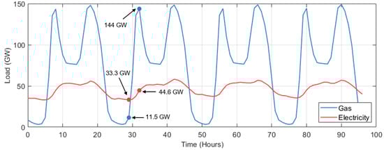
Figure 1. Load seen by the UK’s electricity and gas networks during typical days of winter. Electricity data taken from [28,29]. Gas demand data taken from [30]. Gas demand curve only includes domestic gas usage.

Figure 1 shows two demand curves, one for electricity (red) and one for gas (blue). The electricity demand considers the load on the whole network during selected winter days of 2021 [28,29]. The blue curve represents the aggregated gas demand of the approximately 25 million residential properties connected to the gas network. Most of this gas usage is for space heating purposes. The profile of gas demand was constructed using data from a 2023 study conducted by the Smart Energy Research Lab [30]. The consumption of an average UK dwelling during winter was multiplied by 25 million. The actual load on the gas network is considerably higher than what the curve shows due to commercial and industrial gas usage. We can see that between 5–8 am, the load on the electricity grid increases by approximately 11.3 GW. On the other hand, the load on the gas network increases by around 132 GW during the same 3-h window due to domestic space heating demand. These numbers align well with figures previously reported by Grant et al. [27].

To deal with this enormous and very rapid increase in demand, the gas network stores additional gas during the night by increasing the pressure in the pipelines. This additional gas is available and ready to be dispatched the next morning when demand starts to rise. In contrast, the electricity grid does not have an inherent capacity to store energy.

Even though heat pumps offer seasonal CoPs of ~3 [31,32,33,34], shifting the heat demand from the gas network to the electricity system will place a very significant load on the electricity grid [35,36].

Watson et al. [37] predicted that if 100% of UK homes used electric heat pumps, the annual electricity demand in the country could increase by between 140 and 190 TWh, depending on the types of heat pumps installed and their performance levels. This translates to an increase of approximately 45–60% with respect to current demand. According to the study, the electrification of space heating could increase peak load in the grid by about 60–80 GW, which is an increase of more than 100% with respect to current levels. On the other hand, C. Whalen [38] estimates that switching to heat pumps in 100% of UK homes would increase annual electricity demand by about 35% (additional 100 TWh) while peak load could increase by an additional 78 GW.

Measures to reduce peaks in the demand for heat are key and should be implemented. These include improving households’ thermal insulation, installing thermal storage systems, and adopting flexible heating patterns [39]. Nonetheless, in its current state, the electricity grid does not have the capacity to support the widespread use of heat pumps across the country.

Some studies have shown that decarbonizing the UK electricity system (considering current demand levels and patterns) and moving to a 100% renewable-based supply would need approximately 80 TWh of grid-scale energy storage to deal with the daily, seasonal and year-to-year variations in renewables [40]. If space heating were electrified, the requirement for grid-scale energy storage could be as high as 175 TWh [41].

The upgrades and reinforcements required to electrify domestic space heating and enable the electricity grid to take on the duty currently handled by the gas network are substantial, expensive and lengthy [42]. Analysts have commented that achieving net zero will require a transformation of the electricity grid on a scale unseen since the 1960s [43,44].

Novelty and Objectives

As mentioned, the two main solutions to decarbonize space heating (hydrogen boilers and electric heat pumps) offer attractive advantages, but they also present some important practical challenges. Electrical heat pumps will place a potentially overwhelming load on the electricity grid, and significant grid upgrades will be required to support their use. Furthermore, if space heating were fully electrified, a significant portion of the existing gas network could become an abandoned asset.

On the other hand, hydrogen allows us to continue using the gas network and to use underground caverns for seasonal storage of energy. However, the process of producing, distributing, and combusting hydrogen in boilers has a low overall efficiency.

This paper introduces a novel and promising technology for zero-carbon space heating (High-Performance Heat-Powered Heat Pumps) which aims to overcome the drawbacks of the current low-carbon heating solutions. It uses hydrogen distributed via the gas network as a fuel, but it offers a much higher efficiency than direct combustion in hydrogen boilers thanks to the incorporation of a heat pumping cycle. At the same time, the proposed concept avoids placing a very significant load on the grid and the need for substantial upgrades and reinforcements. The technology presented in this paper has real prospects of accelerating progress towards net zero by improving its affordability.

A full techno-economic assessment of the HP³ system is beyond the scope of this study. The primary objective of the paper is to introduce a novel and interesting zero-carbon heating technology (HP³), describe its operating principles, and explore how different design choices influence the performance of the system. The paper aims to establish the fundamental thermodynamic behavior of the technology and provide the basis for more detailed cost and feasibility assessments once prototype data and refined component designs become available.

The results demonstrate the performance potential of HP³ and highlight its value from a broader energy system integration perspective. The findings of this study provide the foundation for future work involving prototype development and experimental validation, as well as a techno-economic analysis of the concept and a comparison with other existing technologies.

2. The HP³ Concept

High-Performance Heat-Powered Heat Pumps (HP³ for short) combine the best attributes of hydrogen boilers and electrical heat pumps, and simultaneously remove their main drawbacks. This set of technologies has real prospects of being transformational in two different ways: (i) by triggering a step-change in the UK space heating industry towards more sophisticated and much higher-value products and (ii) accelerating the achievement of net zero by improving affordability.

HP³ systems are a type of thermo-mechanical system that blends a heat engine and a heat pump into a single, fully integrated system. These systems take in a small amount of high-grade heat from the combustion of fuel (e.g., hydrogen) and supply a large amount of low-grade heat for space heating.

The deployment of HP³ systems in the country allows the existing gas network—a hugely valuable asset—to continue operating. The gas network can deliver hydrogen (or another clean fuel) to dwellings across the country to meet the demand for heat during the colder months of the year.

The deployment of HP³ systems also opens the possibility of using underground solution-mined caverns [15,16,17,18,19,20,21,22] to stockpile large amounts of hydrogen in preparation for the next winter, similar to what is done with natural gas reserves. Exploiting the gas network and using caverns for seasonal energy storage are advantages not exclusive to HP³ systems. Less sophisticated hydrogen boilers also offer these same benefits. However, due to their heat multiplication effect, HP³ systems maximize the benefit per unit mass of hydrogen, thereby reducing the amount of fuel needed.

As previously mentioned in Section 1, the electrification of space heating in the country will significantly stress the electricity grid. Many believe that without substantial upgrades and reinforcements, the electricity grid will not be capable of sustaining the operation of heat pumps in any significant fraction of UK homes. The use of HP³ systems avoids placing this additional and potentially overwhelming load on the electricity grid as the heating demand continues to be met by the gas network infrastructure.

The technology proposed is not exclusive to a specific fuel and can be adapted to work with any source of high-grade heat. Therefore, it can be deployed before hydrogen is widely distributed through the gas network, reducing the overall consumption of natural gas and associated CO₂ emissions as the country transitions to zero-carbon heating.

HP³ systems achieve a similar heat multiplication effect to that of heat pumps. This translates into a reduced usage of fuel for a given heat output. Figure 2 illustrates how HP³ systems achieve this effect. The heat engine part receives n kWh of energy in the form of high-temperature heat from the combustion of hydrogen. The heat engine transforms this into X kWh of mechanical work and (n − X) kWh of low-grade heat, which is part of the system’s output and is used to provide space heating. The X kWh of work drives the heat pump part of the system.

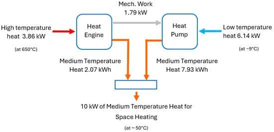
Figure 2. Heat multiplication effect of an HP³ system.

The heat pump extracts a total of X(CoP − 1) kWh of low-grade heat from the surroundings and delivers a total of (X∙CoP) kWh of low-grade heat at a temperature suitable for space heating. The total heat output from the combined system is (n − X) + (X∙CoP). Here, CoP is the coefficient of performance of the heat pump part, which is normally between 1 and 4, and n is a design variable of the heat engine part (related to its efficiency). To illustrate the concept, Figure 2 shows the heat and work flows in a unit with a 10 kW output. Section 3, Section 4, Section 5 and Section 6 discuss in detail how these values have been calculated.

A key distinction between an HP³ system and a conventional heat pump is the form of the input energy. A conventional heat pump consumes electrical energy while an HP³ system is powered by thermal energy.

HP³ systems can be configured in several different ways. Figure 3 shows a design that allows the heat engine and heat pump parts of the system to use a common heat output device (a condenser) and share the same working fluid.

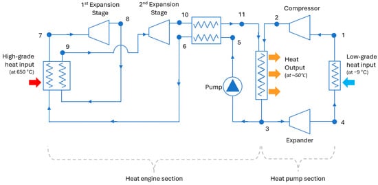
Figure 3. A possible configuration for an HP³ system. The node numbers indicate different states of the working fluid across the system; the text refers to these points.

The heat pump part of the system works in the same way as a normal heat pump. The only difference is that the compressor is driven by the mechanical work produced by the heat engine part and not by electricity. The working fluid passes through an evaporator where it gathers heat from the ambient air and boils (4 → 1). The gaseous fluid is then compressed, which increases its pressure and temperature (1 → 2). After the compressor, the fluid passes through a condenser (common with the heat engine), where it releases its heat content and becomes liquid again (2 → 3). Lastly, an expander reduces the pressure of the fluid so that its temperature falls below ambient (3 → 4) and the cycle can start again. The expansion of the fluid produces some work, which offsets the total work required by the compressor. A throttle or expansion valve could be used here instead of an expander; however, the pressure drop of the fluid will not generate work.

In the heat-engine part of the system, the working fluid enters a heat collector, where it absorbs high-grade heat from the combustion of hydrogen and evaporates (6 → 7). Subsequently, the hot pressurized gas produces mechanical work in an expander (7 → 8). Figure 3 shows a system with two stages of expansion with reheating between them; however, a different number of stages could be employed. After the first expansion (8), the fluid passes again through the high-grade heat collector (8 → 9) where it is brought back to the maximum operating temperature of the system. The working fluid is then further expanded in the second expander (9 → 10).

As mentioned, the mechanical work produced from the expansion of the working fluid in the two stages is used to drive the compressor of the heat pump (and the pump of the heat engine). A shaft (not shown in Figure 3) mechanically links the heat engine’s expander to the heat pump’s compressor. After emerging from the second expander, the fluid passes through a recuperator (10 → 11) where it preheats the low-temperature stream going to the high-grade heat collector (5 → 6).

After the recuperator, the working fluid enters the heat output device (shared with the heat pump) where it releases most of its heat content and condenses (11 → 3). Ideally, the temperatures and pressures at points (11) and (2) would be the same to avoid exergy destruction when the two streams of the working fluid mix in the heat output device. However, allowing a small difference here provides design flexibility.

The working fluid in liquid form (3) is pumped to a high pressure again (5), and the cycle repeats. The heat that is not absorbed by the working fluid in the high-grade heat collector could be recuperated and sent to the low-grade heat output device to minimize losses. The heat output from the condenser is used to produce hot water, which circulates through the heat distribution system of the dwelling.

The operation described assumes the working fluid changes phase from liquid to gas and vice versa in different parts of the system. An all-gas approach is also possible, although the focus of this paper is on cycles and working fluids that involve liquid-gas transitions.

There are heat pumps driven by gas engines (GEHPs), which are another kind of heat-powered heat pumps. In this case, an internal combustion engine burns natural gas to produce mechanical work and drive the compressor of a heat pump. The waste heat of the engine is recuperated and used to provide additional heating [45,46,47,48]. GEHPs are more common in commercial or industrial applications. GEHPs are not very common at a global scale, with Japan and South Korea being the primary global markets. The main difference between a GEHP and the HP³ concept presented here is the level of integration of the system. A GEHP connects the two parts of the system–engine and heat pump–via a mechanical shaft. An HP³ system aims to integrate both parts more tightly into a single system. It accomplishes this by sharing the same working fluid and a common heat output unit, in addition to the main shaft to transfer mechanical power. Combining both subsystems into a single, fully integrated system can lead to better performance and possibly reduce costs. Another unique feature of an HP³ system is the addition of a small electrical motor coupled to the main shaft connecting the heat engine’s expander to the heat pump’s compressor. In addition to starting the system, this motor provides operational flexibility and allows for the power output of the expander to be greater than the power consumed by the compressor. The design of an HP³ system can be seen as a continuum between a pure heat engine and a pure heat pump.

If the design of the system is not balanced and it leans towards being ‘more heat engine’ (i.e., excess work produced by the expander), the motor will generate some electricity at the expense of a reduced low-grade heat output. If designed to be more heat engine, an HP³ system could be regarded as a type of ‘combined heat and power’ (CHP) system. The main difference between the proposed systems and existing micro-CHP plants is the heat-pump cycle, which increases the system’s low-grade heat output.

In the heat engine section, the working fluid can reach temperatures of approximately 650 °C after collecting high-grade heat from the combustion of hydrogen (or another clean fuel). Although this may seem high for a domestic system, current natural gas boilers see temperatures over 1000 °C inside the combustion chamber [49,50]. The difference is that in a gas boiler, hot water is produced directly, and its temperature is not allowed to exceed approximately 70 °C. In an HP³ system, the working fluid is allowed to reach much higher temperatures, but the hot water output will still be under the safe limit. Therefore, from this point of view, implementing an HP³ system in a domestic setting seems feasible. It should be noted that HP³ systems could also be implemented at a larger scale (e.g., district heat networks [51,52]) where a central multi-MW system can combust hydrogen, produce hot water and deliver it to several dwellings.

The capability of the system to generate electrical power is an interesting feature with potential system-level benefits. As the UK decarbonizes, it is likely that a significant fraction of homes will keep warm using electric heat pumps [53]. As discussed, these heat pumps will represent a significant load for the electricity system. Houses where HP³ systems are installed will not use electricity from the grid to meet their heating needs and can also generate some electricity, while heat pumps elsewhere are drawing energy. This energy can be either self-consumed or exported and will reduce the strain on the grid caused by other dwellings across the country using electrical heat pumps.

It is interesting to compare the HP³ technology against electrical heat pumps and gas boilers in terms of CO₂ emissions. The space heating demand of an average UK home is about 10.8 MWh (12 MWh of natural gas × 0.9 boiler’s efficiency) [54]. Burning natural gas produces 0.185 kg of CO₂ per kWh of heat released [55,56,57]; therefore, a domestic gas boiler in the UK emits around 2 metric tons of CO₂ per year [1]. An electrical heat pump and an HP³ system can supply a house’s heat demand while producing 0 kg of CO₂ per year, provided that the electricity or hydrogen consumed comes from a zero-carbon source (i.e., renewables). However, currently this is not the case. A large share of electricity in the UK is still generated from natural gas, and hydrogen supply is not fully green yet.

Let us consider the case of an electrical heat pump first. If the electricity consumed comes from gas-fired generation, approximately 0.4–0.5 kg of CO₂ are produced per kWh of electricity [58]. Considering an average CoP of 3, a heat pump will consume 3.6 MWh of electricity to supply the average house’s annual demand of 10.8 MWh of heat. This translates into ~1.6 tons of CO₂. This would be avoided altogether if electricity were produced by renewables (wind and solar PV).

In the case of an HP³ system, the fuel could be blue hydrogen. Blue hydrogen is generated using the same steam methane reforming (SMR) method as grey hydrogen, but it incorporates carbon capture and storage (CCS) to curb emissions. The CO₂ by-product is collected, compressed, and then either injected into underground storage sites or repurposed for industrial uses. The added CCS greatly lowers the carbon output of hydrogen production, though the exact amount of reduction depends on how effective the capture system is. Typical efficiencies range between 56–90% [59]. Considering these values, between 3.97 and 6.87 kg of CO₂ are emitted per kg of H₂ produced (in addition to what is captured and stored) [60,61]. Considering a calorific value of hydrogen of 142 MJ/kg (39.44 kWh/kg), the above translates to between 0.1 and 0.175 kg of CO₂ per kWh of heat.

Considering an annual heat demand of 10.8 MWh for the average UK property, an HP³ system with a CoP_HP3 of 2.5 will consume 4.32 MWh of heat from hydrogen, equivalent to 109.5 kg of hydrogen per year. Depending on the efficiency of the CCS process used to produce the blue hydrogen, this represents between 430–750 kg of CO₂ per year.

Both electrical heat pumps and HP₃ systems can be zero carbon solutions, but this depends on the energy source. If blue hydrogen or gas-fired electricity is used, CO₂ emissions will be significant and comparable to those of natural gas boilers.

3. Parametric Analysis of the Heat Pump Subsystem

This section presents a parametric investigation for the heat pump part of the HP³ system. Two parameters are used as design variables: $P_{low}$ and $P_{intermediate}$, which are the pressures at the evaporator and at the condenser, respectively. Several combinations of the two variables are assessed.

In this study we use propane (R290) as the working fluid for both parts of the system. Propane is a commonly used fluid in current commercially available heat pumps. It performs well over a wide range of operating conditions (including temperatures up to ~695 °C), is not corrosive, and has a very low Global Warming Potential (GWP) value.

Propane was selected as the working fluid because, in addition to being commonly used in heat pumps, preliminary assessments showed that it could also perform well under the very different set of operating conditions in the heat engine part (discussed in Section 4). Other fluids offering some attractive features were explored, such as argon, carbon dioxide, and ammonia. However, none were able to perform well under both sets of conditions. An HP³ arrangement allowing the use of two separate fluids for the two subsystems was also considered. Steam was evaluated as the fluid for the heat engine and a typical refrigerant for the heat pump part. However, this configuration departs from the integrated design approach targeted in this study, which aims for a shared condenser. Therefore, propane was selected as the working fluid.

The performance of the heat pump part of the system is calculated on a per-unit mass basis, using a flow rate of 1 kg/s. The mass flows in both parts of the system (heat engine and heat pump) need to be determined jointly to ensure that (1) the shaft power of the heat engine expander is enough to drive the compressor of the heat pump and (2) the overall heat output of the full system matches the requirement.

Ambient temperature is set to −9 °C, which is a pessimistic scenario. Average winter temperatures in the UK are typically between 2 °C and 7 °C, with minimums often dropping to slightly below 0 °C. However, maintaining good performance levels during extreme weather events is important because it is precisely at these times that heating demand will see the biggest peaks.

In this study we consider a hydronic heating system. That is, the HP³ system will produce hot water which is distributed through a circuit of pipes to provide space heating via an array of radiators. The flow temperature (i.e., the temperature at which the water leaves the heating system) has a lower limit of 45 °C. This is also common in domestic heat pump installations [62]. In this study, the upper limit for the flow temperature is not fixed and depends on specific design choices. However, higher flow temperatures lead to reduced coefficients of performance (CoP). A standard return temperature of 35 °C is assumed.

A model of the heat pump section was implemented in MATLAB R2021a. The MATLAB model is linked to REFPROP, a fluid thermodynamic properties database developed by NIST [63,64]. Table 1 provides a summary of the assumptions made in the model.

Table 1. List of the assumptions made for the modeling of the heat pump subsystem.

Assumptions for the Heat Pump Modeling

Real gas properties of the working fluid (R290) obtained from REFPROP No chemical reactions or decomposition of the working fluid. Steady-state operation (no transient effects). Negligible pressure drops in evaporator, condenser and pipes No pressure drops during compressor’s suction and discharge No heat losses to the environment Fully developed flow regimes for the working fluid Constant ambient temperature (−9 °C) Working fluid is 5° colder than ambient when emerging from evaporator Fixed return temperature of 35 °C for the water loop Fixed condensing temperature of 40 °C Steady mass flow rates of the working fluid No auxiliary loads (fans, pumps, defrost heaters, etc.) Work is recovered from expansion device, with an isentropic efficiency of 80% Compressor has an isentropic efficiency of 80% Changes in kinetic or potential energy of the working fluid have no effect on the energy balance

Let us look at point (1), which is just after the evaporator and before the compressor (see Figure 3). The temperature at this point (T₁) is set to be 5 °C lower than ambient temperature. This temperature difference allows good heat transfer in the evaporator without requiring a very large area. T₁ must remain above the saturation temperature at $P_{low}$ so that the fluid can evaporate after collecting low-grade heat from ambient. Entropy (S₁) and enthalpy (H₁) values are given by REFPROP.

Pressure at point (2) is equal to $P_{intermediate}$. We start the calculation by considering a fully isentropic compression; the actual conditions are calculated in the next step. Therefore S₂′ is equal to S₁. Knowing values for entropy (S₂′) and pressure (P₂), the values of T₂′ and H₂′ can then be obtained from REFPROP.

The real value for the enthalpy of the fluid at point (2) is calculated by means of Equation (1), which accounts for the real isentropic efficiency of the compressor (${\eta }_{comp}$). The compressor of the heat pump has a target efficiency of 80%.

$$H_2={\displaystyle \frac{{H_2}^{\prime }-H_1+(H_1\times {\eta }_{comp})}{{\eta }_{comp}}}$$

(1)

After calculating H₂, the real values for the entropy (S₂) and temperature (T₂) of the fluid at point (2) can be found from REFPROP.

Point (3) is immediately after the condenser. The pressure here is equal to $P_{intermediate}$. The temperature at this point is set to 40 °C, which is 5 °C higher than the water return temperature. This temperature difference is commonly used and allows for effective heat transfer in the condenser. Since P₃ and T₃ are known, the entropy and enthalpy of the fluid can be found via REFPROP.

T₃ must remain below the saturation temperature at P₃ to ensure condensation. This maximizes the amount of heat that can be removed per unit mass.

Lastly, point (4) is situated before the evaporator but after a pressure-reduction device. Here, pressure is equal to $P_{low}$. The pressure-reduction device can be a throttle or an expansion valve, which removes pressure from the liquid working fluid without producing work. Alternatively, it can be an expander which produces work from the fluid’s pressure drop.

Throttling is an isenthalpic process; heat transfer is negligible, and no work is done. Therefore, H₄ = H₃ if a throttle is used. Knowing P₃ and H₄, we can query REFPROP to find the entropy (S₄) and temperature (T₄) of the fluid.

If an expander were used, then S₄′ = S₃. The values of T₄′ and H₄′ can be obtained from REFPROP. The real enthalpy of the fluid at point (4) is calculated by means of Equation (2), which considers the effect of the isentropic efficiency of the expander.

$$H_4=H_3-{\eta }_{expand}\times (H_3-{H_4}^{\prime })$$

(2)

After having calculated H₄, the real values for the entropy (S₄) and temperature (T₄) of the fluid can be found via REFPROP.

In this paper we consider the use of an expander between points (3) and (4), which means that work is produced. This improves the CoP of the heat pump and reduces the work required from the heat engine. The study assumes isentropic efficiencies of 80% for the compressor and expander of the heat pump.

The rate of heat extraction from the low-grade source is given by Equation (3), while the output of the heat pump can be calculated through Equation (4). In the equations, $\dot{m}$ is the mass flow of working fluid through the heat pump.

$$Hea{t}_{In}=\dot{m}\times (H_1-H_4)$$

(3)

$$Hea{t}_{out}=\dot{m}\times {(H}_2-H_3)$$

(4)

The work consumed by the compressor is calculated by means of Equation (5) while the work produced by the expander is given by Equation (6). As mentioned, if a throttle were used, H₃ = H₄ and $W_{expand}$ is zero. The net work consumed by the heat pump section is the difference between these two quantities. This is the amount of work that the heat engine needs to produce in order to drive the system.

$$W_{\mathit{comp}}=m\times (H_2-H_1)$$

(5)

$$W_{\mathit{expand}}=m\times (H_3-H_4)$$

(6)

W_net − ℎeatpump = W_comp − W_expand

(7)

The coefficient of performance (CoP) of the heat pump is defined as the ratio between the heat output and the net work consumed, as shown in Equation (8):

$$Co{P}_{heatpump}={\displaystyle \frac{Hea{t}_{out}}{W_{net}}}$$

(8)

Figure 4 shows how the CoP of the heat pump changes with respect to the two design variables: the evaporator pressure ($P_{low}$) and the condenser pressure ($P_{intermediate}$). It can be seen that for any given value of $P_{low}$, the CoP increases as $P_{intermediate}$ approaches the saturation pressure of propane at T₃ (13.7 bar, 40 °C).

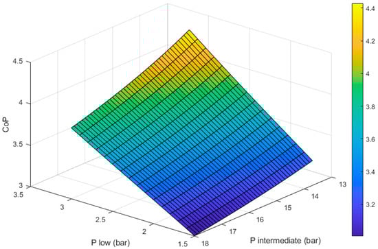
Figure 4. Coefficient of performance of the heat pump section with respect to the evaporator ($P_{low}$) and condenser ($P_{intermediate}$) pressures. T₃ = 40 °C; T_amb = −14 °C.

Compressing beyond 13.7 bar will lead to higher compressor outlet temperatures (T₂). This could be beneficial if a higher flow temperature is desired; however, it translates into more compression work, leading to a reduced CoP.

If the compressor’s outlet pressure is below 13.7 bar, the gaseous working fluid will not become liquid in the condenser. This significantly reduces the heat output per unit mass of working fluid.

We can also see in Figure 4 that the CoP is maximized as the value of $P_{low}$ approaches the saturation pressure of propane at T₁ (3 bar, −14 °C). If the pressure in the evaporator is higher than ~3 bar, the fluid will not boil, which limits the amount of heat it can extract from ambient per unit mass of working fluid. Additionally, if the working fluid is liquid, the compressor will not be able to raise its temperature to the required levels to provide space heating.

For any given value of $P_{intermediate}$, a lower $P_{low}$ will increase the compression ratio ($P_{intermediate}/P_{low}$), which translates into more work being done by the compressor. The work produced by the expander will increase as $P_{low}$ reduces but not in the same proportion. The net effect of this is that lower values of $P_{low}$ lead to reduced CoPs, as shown in Figure 4.

Figure 5 shows how the temperature at the outlet of the compressor (T₂) varies with respect to its inlet and outlet pressures.

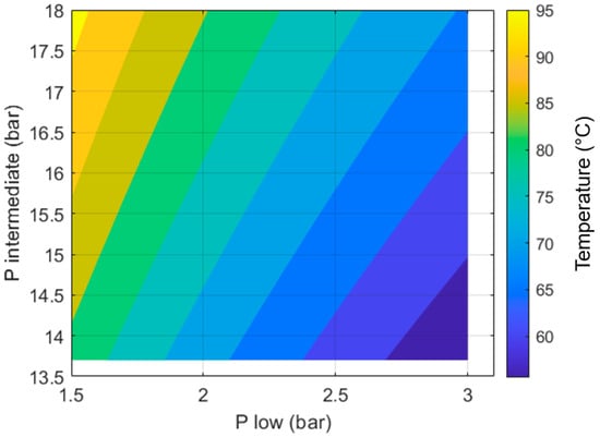
Figure 5. Variation in the compressor’s outlet temperature (in °C) with respect to inlet and outlet pressure.

As we can see in Figure 4, the maximum CoP achievable is ~4.43. This is achieved with a $P_{low}$ of 3 bar, which matches the saturation pressure at −14 °C, and a $P_{intermediate}$ of 13.7 bar, which matches the saturation pressure at 40 °C.

In this configuration, the work done by the compressor is 82.32 kW per kg of working fluid while the expander produces 12.26 kW per kg of working fluid. If instead of an expander a throttle were used, the CoP of the heat pump would fall to 3.82. The net work consumed is higher for the same heat output.

As mentioned, ambient temperature has been set to −9 °C. However, the CoP of the heat pump would improve if the temperature of the low-grade heat source were not as cold. For example, if ambient temperature were 0 °C (T₁ = −5 °C), the CoP would increase by ~20% to 5.32. $P_{intermediate}$ is kept the same but $P_{low}$ would increase to 4.06 bar to match the saturation pressure of the fluid at the new T1. This reduces the work done by the compressor and thereby the CoP increases.

4. Parametric Analysis of the Heat Engine Subsystem

This section addresses the design of the heat engine subsystem of the HP³ system. A parametric exploration is carried out with two design variables: (1) the pressure of the working fluid at the high-grade heat collector ($P_{high}$) and (2) the temperature of the fluid at the outlet of the high-grade heat collector ($T_{max}$). For $P_{high}$, a range of values between 40–350 bar is evaluated. For $T_{max}$, a range of 250 °C to 700 °C is considered. Several combinations between these two variables are assessed. Table 2 provides a summary of the assumptions made by the model.

Table 2. List of the assumptions made for the modeling of the heat engine subsystem.

Assumptions for Heat Engine Modeling

Real gas properties of the working fluid (R290) obtained from REFPROP No chemical reactions or decomposition of the working fluid. Steady-state operation (no transient effects). Negligible pressure drops in high-grade heat collector, recuperator, condenser and pipes No heat losses to the environment Fully developed flow regimes. Working fluid is at specified temperature at outlet of combustion chamber Fixed condensing temperature of 40 °C Steady mass flow rates of working fluid Pump has a fixed efficiency of 80% Recuperator has an effectiveness of 97% No other auxiliary loads Isentropic efficiency of expanders is set to a target of 80% Changes in kinetic or potential energy of the working fluid have no effect on the energy balance

As mentioned, the heat engine shares a common heat output device (i.e., the condenser) with the heat pump. Therefore, on the heat engine side, the fluid’s pressure at the inlet of the condenser (P₁₁) is set to be the same as the outlet pressure of the heat pump’s compressor (P₂). This allows the working fluid to condense at the same temperature (40 °C) as in the heat pump.

On the heat engine side, the temperature of the fluid at the inlet of the condenser (T₁₁) should be equal to the outlet temperature of the heat pump’s compressor (T₂). Exergy destruction would be minimized if the two streams of working fluid entering the condenser had the same temperatures and pressures. However, fixing the temperature at this point over constrains the design of the heat engine. In this study, this temperature (T₁₁) is a result of design choices and not an input.

Operating conditions at point (3) are common with the heat pump section and known. Here, the fluid is in liquid form at the saturation pressure corresponding to a temperature of 40 °C.

In point (5), a pump raises the pressure of the liquid working fluid to $P_{high}$. The pump is assumed to have an isentropic efficiency (${\eta }_{pump}$) of 80%.

Because this is an (almost) isentropic compression process, S₅′ is equal to S₃. Knowing P₅ and S₅′ we can find values for T₅′ and H₅′ via REFPROP. The real value for the enthalpy of the fluid (H₅) is calculated by means of Equation (9):

$$H_5={\displaystyle \frac{{H_5}^{\prime }-H_3+({\eta }_{pump}\times H_3) }{{\eta }_{pump}}}$$

(9)

Subsequently, the real values for the temperature (T₅) and entropy (S₅) of the fluid at point (5) can be found. Next, we move to point (7) which is located at the outlet of the high-grade heat collector. Here, the pressure of the fluid is $P_{high}$ and its temperature is $T_{max}$. The entropy (S₇) and enthalpy (H₇) of the fluid are found by querying REFPROP.

Point (8) is located after the first stage of expansion. Here, the pressure of the fluid has reduced from $P_{high}$ down to some pressure between $P_{high}$ and $P_{intermediate}$ (condenser pressure). The expander produces mechanical work from this pressure drop.

The pressure after the first expander (P₈) can be calculated by means of Equation (10). The two expansion stages are assumed to have the same pressure ratio.

$$P_8=P_{intermediate}\times \sqrt{{\displaystyle \frac{P_{high}}{P_{intermediate}}}}$$

(10)

Expansion is an isentropic process; however, it is not 100% efficient. Therefore, S₈′ = S₇. Using REFPROP, the values of H₈′ and T₈′ are obtained. Subsequently, the real enthalpy of the fluid at point (8) is calculated through Equation (11):

$$H_8=H_7-{\eta }_{expand}\times (H_7-{H_8}^{\prime })$$

(11)

Then, the real values for the temperature (T₈) and entropy (S₈) of the fluid are obtained from REFPROP. After the first expansion, the fluid is recirculated through the high-grade heat collector, where it is reheated to the maximum operating temperature of the system ($T_{max}$). The temperature and pressure of the fluid at point (9) are known. Its entropy and enthalpy can be found from REFPROP.

The fluid produces further mechanical work in the second expansion stage (point 10). Here, the pressure is $P_{intermediate}$. Given that the process is not 100% efficient, S₁₀′ = S₉. REFPROP is used to find T₁₀′ and H₁₀′. The actual enthalpy (H₁₀) is calculated through Equation (12). Following that, the real temperature (T₁₀) and entropy (S₁₀) values can be found using REFPROP.

$$H_{10}=H_9-{\eta }_{expand}\times (H_9-H_{10}^{\prime })$$

(12)

After exiting the second expansion stage, the fluid still holds a considerable amount of heat. A recuperator is used to extract this energy to preheat the fluid stream going to the high-grade heat collector. This recuperator increases the overall efficiency of the system.

The inlet conditions of the recuperator are known: temperature, pressure, entropy and enthalpy at points (5) and (10). The mass flow has not been determined yet, but both streams have the same mass flow since the system is a closed loop.

Let us call the stream of fluid flowing from point (10) to point (11) the “hot” stream, where T₁₀ = $T_{hot\text{-}inlet}$ and T₁₁ = $T_{hot\text{-}outlet}$. We will call the stream flowing between points (5) and (6) the “cold” stream, where T₅ = $T_{cold\text{-}inlet}$ and T₆ = $T_{cold\text{-}outlet}$.

Determining the two outlet temperatures requires an iterative loop. We take initial guesses for the two outlets. Initially $T_{hot\text{-}outlet}$ is assumed equal to $T_{cold\text{-}inlet}$; the real value will be higher. $T_{cold\text{-}outlet}$ is assumed equal to $T_{hot\text{-}inlet}$; the real value will be lower. Enthalpies at the outlet are determined using REFPROP with the guessed outlet temperatures.

Then, for the hot stream, we calculate the temperature and enthalpy changes, as shown in Equations (13) and (14):

$$∆T_{hot}=abs (T_{hot\text{-}inlet}-T_{hot\text{-}outlet})$$

(13)

$$∆H_{hot}=abs (H_{hot\text{-}inlet}-H_{hot\text{-}outlet})$$

(14)

The specific heat capacity ($C_p$) of the fluid is defined as the ratio between the change in enthalpy and the change in temperature, as Equation (15) shows.

$$C{p}_{hot}={\displaystyle \raisebox{1ex}{$∆H_{hot}$}\!\left/ \!\raisebox{-1ex}{$∆T_{hot}$}\right.}$$

(15)

The $∆T$, $∆H$ and $C_P$ for the cold stream are calculated in a similar way. The thermal masses of both streams ($C_{hot}$ and $C_{cold}$) are the product of the mass flow and the specific heat capacity of each stream. In this case both streams have the same mass flow. For now, a flow of 1 kg/s will be assumed.

The maximum heat transfer possible ($Q_{max}$) is calculated as Equation (16) shows. The smallest of the two thermal masses is the limiting factor

$$Q_{max}=\Psi \times (T_{hot\text{-}inlet}-T_{cold\text{-}inlet})$$

(16)

$$\Psi =min (C_{cold}, C_{hot})$$

(17)

Knowing the maximum possible heat transfer, revised values for the outlet temperatures of the hot and cold streams can be calculated by means of Equations (18) and (19), respectively. In the equations, the effectiveness of the heat exchanger is represented by $\epsilon$. We assume this to be 97%.

$$T_{hot\text{-}outlet}=T_{hot\text{-}inlet}- {\displaystyle \frac{(\epsilon \times Q_{max})}{C_{hot}}}$$

(18)

$$T_{cold\text{-}outlet}=T_{cold\text{-}inlet}+{\displaystyle \frac{(\epsilon \times Q_{max})}{C_{cold}}}$$

(19)

Then, the outlet enthalpies of both streams are found using REFPROP. The real enthalpy changes in the two streams are calculated as follows:

$$∆H_{hot}= H_{hot\text{-}outlet}-H_{hot\text{-}inlet}$$

(20)

$$∆H_{cold}= H_{cold\text{-}outlet}-H_{cold\text{-}inlet}$$

(21)

Typically, this loop takes a small number of iterations to converge (<10). Once convergence has been reached, the enthalpy gained by the cold fluid ($∆H_{cold})$ is the same as the enthalpy lost by the hot fluid ($∆H_{hot})$. The enthalpy change in the fluid corresponds to the actual heat transfer rate ($Q_{max} \times \epsilon )$.

After the iterative calculation of the recuperator has finished, the outlet conditions T₁₁, H₁₁, T₆ and H₆ are known. This concludes the calculation of the working fluid’s conditions at all points in the heat engine section.

The mechanical work produced by the first and second stages of expansion can be calculated by means of Equations (22) and (23). In the equations $\dot{m}$ is the mass flow of working fluid. The total work produced by the heat engine is the sum of these two quantities.

$$W_{stage1}=\dot{m}\times (H_8-H_7)$$

(22)

$$W_{stage2}=\dot{m}\times (H_{10}-H_9)$$

(23)

$$W_{output}=W_{stage1}+W_{stage2}$$

(24)

The work done by the pump to raise the pressure of the fluid is calculated via Equation (25). The net work output of the heat engine section is the difference between the shaft work of the two expanders and the work done by the pump.

$$W_{pump}= \dot{m}\times (H_5-H_3)$$

(25)

$$W_{net\text{-}engine}= W_{output}-W_{pump}$$

(26)

As mentioned, the working fluid passes twice through the high-grade heat collector. The total high-grade heat input to the system is given by Equation (27). The heat engine’s heat output is calculated as shown in Equation (28).

$$Q_{input}= \dot{m}\times \left[ \left(H_7-H_6\right)+\left(H_9-H_8\right) \right]$$

(27)

$$Q_{output}=\dot{m}\times (H_{11}-H_3)$$

(28)

There must be an energy balance within the heat engine section. The net work output ($W_{net\text{-}engine}$) plus the heat output ($Q_{output}$) must be equal to the total high-grade heat input ($Q_{input}$).

The mass flow required for either part of the system, heat pump and heat engine, must be calculated simultaneously in an iterative loop. For every combination of design parameters of the heat engine ($P_{high}$ and $T_{max}$) there will be a set of two mass flows, one for the heat pump, one for the heat engine.

Two conditions must be met: (1) the total heat output of the system, which is partly provided by the heat pump and partly provided by the heat engine, must be equal to a set value (e.g., 10 kW). (2) The heat engine’s net power output must match the heat pump’s required power. This condition applies in the case where the system is “balanced”. As mentioned in Section 2, an HP³ system can be designed to be “more heat engine”. In such cases, the net power output of the heat engine must be enough to drive the heat pump and to generate the desired amount of electricity.

As an illustrative example, let us consider a heat output capacity of 10 kW for the full HP³ system. This is a typical size for a domestic electric heat pump in the UK. The coefficient of performance of the full system ($Co{P}_{HP3}$) is defined as shown in Equation (29):

$$Co{P}_{HP3}={\displaystyle \frac{Full System Heat Output}{Heat Engine Heat Input}}$$

(29)

Figure 6 shows how the CoP_HP3 of a full HP³ system varies with respect to the two design variables of the heat engine: the outlet temperature of the high-grade heat collector ($T_{max}$) and the inlet pressure of the first expansion stage ($P_{high}$). The heat pump part of the system is already optimized (as described in Section 3) for an ambient temperature of −9 °C and a condensing temperature of 40 °C. The CoP of the heat pump part of the system does not vary with respect to $T_{max}$ or $P_{high}$ and stays constant at 4.43.

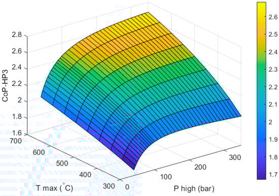
Figure 6. Effect of the maximum temperature and pressure of the heat engine on the CoP_HP3 of the full HP³ system.

As expected, increasing the values of $T_{max}$ and $P_{high}$ leads to higher CoP_HP3. It should be noted that the calculation of the CoP_HP3 is independent of the size of the system. Although from a performance point of view it is desirable to increase the temperature and pressure of the working fluid as much as possible before expansion, there are also some practical considerations. High operating temperatures and pressures increase risks which lead to higher system costs. Additionally, working fluids have operating temperature limits above which they dissociate. Propane begins to decompose around 697 °C [65]. A study by Lifshitz and Frenklach showed that at temperatures about 775 °C propane still has a concentration close to 100% and the concentration of the products is almost zero [66]. The product formation rate increases very rapidly at temperatures above 920 °C [65,66].

Based on the above, in this study we have chosen a “best” design based on a $P_{high}$ of 250 bar and a $T_{max}$ of 650 °C. At this temperature propane is still stable. This design achieves a CoP_HP3 of 2.591. A better performance could be achieved by increasing the maximum pressure of the system but without a formal cost analysis, this is deemed a good compromise between performance and feasibility. For comparison, gas-engine heat pumps (GEHP) typically achieve full system CoPs between 1.5–1.8 (this is often referred to as the primary energy ratio or PER) [45,46,47,48].

As mentioned in Section 2, a temperature of 650 °C is manageable for a domestic system; for context, the combustion chamber of a natural gas boiler sees much higher temperatures [49,50]. The maximum system pressure ($P_{high}$) is also high and can raise questions about the feasibility and safety of the concept. The authors consider pressures higher than 250 to be unfeasible due to increased costs and perceived risks. Therefore, we have selected this design combination ($P_{high}$ of 250 bar and a $T_{max}$ of 650°) and decided to not use a higher temperature or pressure even though performance would improve.

The ASME boiler and pressure vessel code provides allowable stresses for stainless steels working at elevated temperatures. At 650 °C, a 304 H stainless steel (a common fabrication material) can support a stress of 417 bar [67]. The code provides values up to 825 °C, suggesting that much higher operating temperatures are possible. For context, gas turbines can operate at inlet pressures of 140–180 bar and inlet temperatures exceeding 1400 °C [68].

For example, a 304 H pipe with an outer radius of 5 mm would need a wall thickness of 3 mm to hold a pressure of 250 bar considering the reduced allowable stress of the material due to the elevated temperature (Barlow equation). This gives some perspective on feasibility. In practice, an array of several smaller tubes could be used, which would reduce the thickness needed and improve heat transfer. Considering this single pipe and a mass flow of working fluid of about ~5.5 × 10⁻³ kg/s (discussed in more detail further on) we find that the flow still sees a relatively low velocity of <3 m/s, which does not represent a challenge. Figure 7 shows the net work output of the heat engine ($W_{net\text{-}engine})$. In all cases, $W_{net\text{-}engine}$ is equal to the work required by the heat pump section. We can see in the figure that the net work output of the heat engine increases with increasing values of $P_{high}$ and $T_{max}$ despite the reduction in mass flow. This reduction controls the work output of the heat engine and ensures it matches the amount required to drive the heat pump.

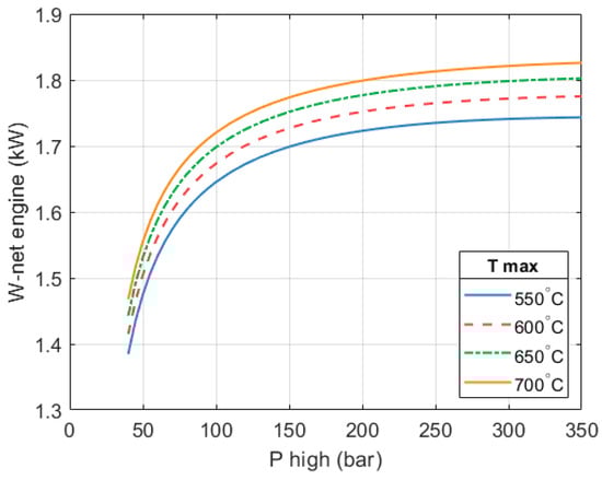
Figure 7. Relationship between the net work output of the heat engine and the two design variables ($P_{high}$, $T_{max}$). A 10 kW system is being considered.

It can also be seen in the figure that for any given level of $T_{max}$, the increase in the work output of the heat engine becomes progressively smaller as the pressure increases beyond 200 bar.

Figure 8 shows how the efficiency of the heat engine section varies with respect to the design parameters. Efficiency is measured as the ratio of the (net) work output to the high-grade heat input. We can see that the efficiency of the heat engine improves as $P_{high}$ and $T_{max}$ increase, which is the reason why the mass flow reduces; more work is produced per unit mass of fluid.

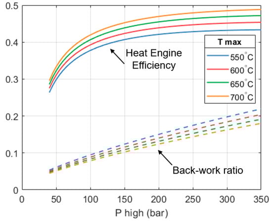
Figure 8. The heat engine’s efficiency (solid lines) and back work ratio (dashed lines) with respect to the maximum temperature and pressure of the system.

An improvement in the efficiency of the heat engine is beneficial for the full system because the heat output of the heat engine reduces, allowing the heat pump part to supply a greater fraction of the total output of the system. Given the high CoP of the heat pump part, increasing its contribution will increase the CoP_HP3 of the overall system.

Figure 8 also shows how the back work ratio (β) of the heat engine varies. The back work ratio is the fraction of the expander’s shaft work that is consumed by the pump. Minimizing β helps to maximize $W_{net\text{-}engine}$. In Figure 8 we can see that β increases as the pump’s outlet pressure increases. On a per unit mass basis, the expanders produce more work as $P_{high}$ increases. However, the work done by the pump also increases. On the other hand, β reduces as $T_{max}$ increases. This is because the expanders can produce more work per unit mass, but the work done by the pump remains constant.

For the design selected (250 bar, 650 °C), the heat engine achieves an efficiency of 46.4%, whilst the observed back work ratio (β) is approximately 15.3%. This is considerably higher than what is seen in typical steam turbines in Rankine cycles, where back work ratios are less than 1%.

The reason for this difference is mainly due to the properties of propane. For example, pumping 1 kg of propane at 40 °C from 13.7 bar up to 250 bar takes 60.3 kW of work. For the same conditions, pumping 1 kg of water takes 29.6 kW of work.

Figure 9 shows how the mass flows of the heat engine and the heat pump parts of the system vary with respect to maximum operating pressure and temperature.

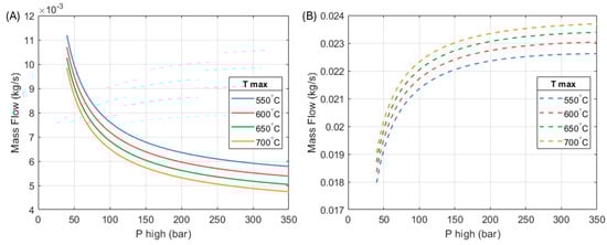
Figure 9. Mass flows through the (A) heat engine and (B) heat pump parts of the HP³ system. A total heat output of 10 kW is considered.

As mentioned, the efficiency of the heat engine improves as the inlet temperature and pressure of the expanders increase. This means that a greater amount of work is produced per unit mass of fluid. The mass flow of the heat engine reduces so that its work output matches the heat pump’s requirement.

On the other hand, as the heat engine becomes more efficient its heat output reduces. In order to maintain the specified system’s heat output (10 kW in this example), the mass flow in the heat pump part increases. In the chosen design (250 bar, 650 °C), the ratio between the mass flow through the heat pump part is approximately 4.34 times the mass flow through the heat engine section.

As the mass flow of the heat pump increases, so does its contribution to the total heat output of the full system. Figure 10 shows how the fraction of the system’s heat output provided by the heat pump changes as $P_{high}$ and $T_{max}$ increase. At a $P_{high}$ of 250 bar and a $T_{max}$ of 650 °C, the heat pump provides 79.3% of the system’s total heat output. The heat engine provides the remaining 20.7%. Because the CoP of the heat pump is much higher, maximizing its contribution improves the overall CoP_HP3 of the system.

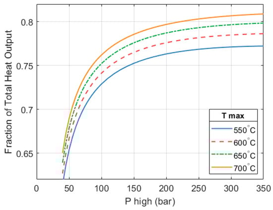
Figure 10. Fraction of the HP³ system’s total heat output that is provided by the heat pump part.

The configuration presented in this paper considers two stages of expansion in the heat engine. This certainly adds complexity and some additional cost to the system, but the gains in performance compensate for this. Using the same operating parameters (a $P_{high}$ = 250 bar and a $T_{max}=$650 °C), a one-stage system would only achieve a CoP_HP3 of 1.54, compared to the 2.591 of a 2-stage system.

The reason for this is that by not re-heating between stages, the efficiency of the heat engine reduces significantly from around 0.47 to about 0.15. This translates into less work produced and a higher heat output. Both effects cause a reduction in the mass flow of the heat pump. The mass flow across the heat pump reduces in order to: (1) decrease the work needed to drive the compressor and ensure the heat engine can drive the system; (2) reduce the heat output of the heat pump to maintain the overall heat output of the HP³ system at the desired level (e.g., 10 kW). In turn, this means that the fraction of the total heat output that is provided by the heat pump part reduces, going from ~79% in a 2-stage system down to approximately 45% in a one-stage system. A smaller contribution of the heat pump part negatively impacts the CoP_HP3 of the full system.

5. Modelling Expansion Efficiency

The previous sections described the modelling and optimization (through a parametric analysis) of the heat pump and heat engine parts of an HP³ system. A 10 kW system was used as an example.

In the calculations, the two expanders (and the pump) of the heat engine were assumed to have an isentropic efficiency of 80%. In this section we introduce a model that allows calculating the efficiency and rotational speed of an expander based on its operating conditions, namely the mass flow ($\dot{m}$), inlet temperature ($T_{in}$), inlet pressure ($P_{in}$) and outlet pressure ($P_{out}$). We use this model to assess whether a target efficiency of 80% is achievable.

As mentioned, propane is being used as the working fluid on both parts of the system. The specific gas constant ($R$) of propane is 189 J/kg-K. In this model we use a constant specific heat capacity ($C_p$) of 1449 J/kg-K. For propane, the ratio between specific heats ($\gamma$) is 1.15.

We will focus on the first stage of expansion. The density of the gaseous propane at the inlet of the expander is calculated via Equation (30), while Equation (31) gives the volume flow rate (m³/s).

$${\rho }_{in}={\displaystyle \frac{P_{in}}{R\times T_{in}}}$$

(30)

$${\dot{V}}_{in}={\displaystyle \frac{\dot{m}}{{\rho }_{in}}}$$

(31)

Calculating the isentropic efficiency of the expander requires an iterative loop. An initial guess is that $T_{out}$ is equal to the inlet temperature and that the efficiency has a low value (e.g., 10%).

The density and volume flow rate at the outlet conditions can be calculated using Equations (30) and (31). The stagnation enthalpy change can be calculated by means of Equation (32), where $r$ is the pressure ratio across the expander and $\eta$ is the assumed isentropic efficiency.

$$∆H_{stag}=C_p\times \eta \times \left(T_{in}-\left( r^x\times T_{in}\right)\right)$$

(32)

$$r={\displaystyle \frac{P_{out}}{P_{in}}}$$

(33)

$$x={\displaystyle \frac{\gamma -1}{\gamma }}$$

(34)

Equation (35) calculates the isentropic efficiency ($\eta$) of the expander with respect to a factor $\phi$, which encompasses the rotational speed ($\omega$—in revolutions per minute), volume flow rate as well as the change in stagnation enthalpy ($∆H_{stag})$

$$\eta =1.007e^{-0.2761\times \phi } -0.9162e^{-7.084\times \phi }$$

(35)

$$\phi = {\displaystyle \frac{\omega \times (2 \pi /60)\times \sqrt{\frac{{\dot{V}}_{in}+{\dot{V}}_{out}}{2}}}{ {∆H_{stag}}^{0.75}}}$$

(36)

The temperature of the working fluid at the outlet of the expander is calculated via Equation (37):

$$T_{out}= T_{in}-\left[T_{in}\times (1-r^x)\times \eta \right]$$

(37)

Once $\eta$ and $T_{out}$ are known, another iteration is carried out. This process usually converges after a small number of iterations.

A MATLAB function was developed around this model. This function allows calculating the rotational speed required to achieve a target isentropic efficiency (e.g., 80%) based on a given set of operating conditions ($\dot{m}$, $T_{in}$, $P_{in}$ and $P_{out}$).

As mentioned, the focus is on the first expander. The same iterative loop can be carried out for the second expander, which has the same pressure ratio but a lower inlet temperature. Generally, the efficiency of the second stage is a few percentage points higher than that of the first stage.

A parametric exploration was carried out using the model and functions discussed. The results are shown in Figure 11. There are four sets of curves representing different mass flows (in different colors). Each set comprises 3 lines (solid, dashed, dash-dotted). Each line considers a different inlet temperature. Target isentropic efficiency is set to 80%. We can see that the rotational speed needed to reach the target efficiency increases with inlet pressure and temperature. Increasing $P_{in}$ and $T_{in}$ is desirable because the heat engine can produce more shaft work per unit mass of working fluid. This leads to a better CoP_HP3 of the full system; however, maintaining the efficiency of the expander becomes more challenging because it needs to turn faster.

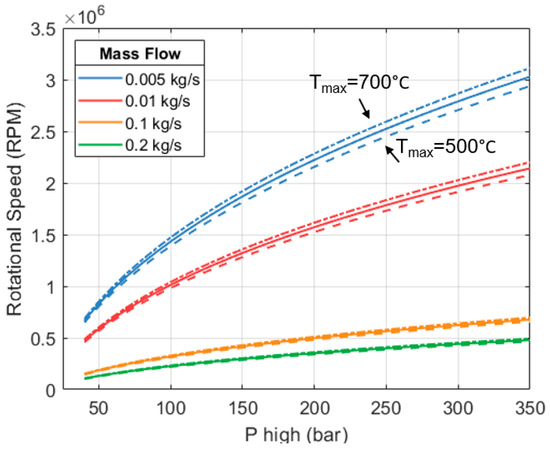
Figure 11. Rotational speed required to maintain a target isentropic efficiency of 80%.

Many combinations of pressures and temperatures within the range explored need rotational speeds > 1 million revolutions per minute (RPM) to achieve an efficiency of 80%. For a space heating system, either at a domestic or industrial scale, this is deemed to be exceedingly high.

We can also see in Figure 11 that for any given combination of $P_{in}$ and $T_{in}$, the rotational speed reduces as the mass flow increases. As the expander becomes physically larger, it does not need to rotate as fast to maintain the same efficiency. This can be used as a mechanism to keep the RPM below a certain limit. However, increasing the mass flow translates into greater heat and work outputs. This only increases the overall size and capacity of the full HP³ system.

In this study we limit the rotational speed ($\omega$) of the heat engine’s expanders to 170 k RPM. For context, automotive turbochargers rotate between 80,000 and 200,000 RPM [69,70], and in some cases, the inlet temperatures of these turbochargers exceed those considered here. Therefore, a speed of 170 k RPM seems reasonable for the expanders of an HP³ system.

Automotive turbochargers have a service life of ~150,000 miles, which is equivalent to approximately 10–12 years [71,72]. We can expect the expander of an HP³ system operating at a similar rotational speed to have a similar lifespan. In the UK, the heating period is typically from October to March. In regions where heating systems are on for shorter periods, a longer service life can be expected.

It should be noted that there are no commercial off-the-shelf expanders for these operating conditions. Although the operating parameters are feasible as we have established, most of the available equipment comes from gas turbines, which use combustion gases as the working fluid instead of propane.

Lower rotational speeds might lead to cheaper machines at the expense of a lower isentropic efficiency. Figure 12 shows how the expansion efficiency changes with respect to the rotational speed of the machine. The illustration considers a mass flow rate of 0.1 kg/s and two stages of expansion with a final pressure of 13.7 bar (pressure at the system’s condenser). The figure only shows the efficiency of the first expander.

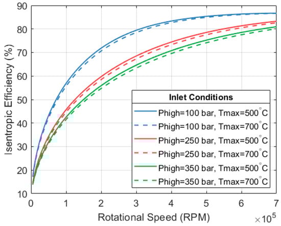
Figure 12. Isentropic expansion efficiency with respect to rotational speed. A mass flow of 0.1 kg/s is considered, with expansion in 2 stages down to 13.7 bar.

Integrating the expander model presented in this section with the full HP³ model allows determining the heat engine mass flow that achieves an 80% isentropic efficiency at the expanders (with 170 k RPM), for a given set of design parameters ($P_{high}$ and $T_{max}$). The optimum pressures of the heat pump part have already been established (as discussed in Section 3). The mass flow in this part of the system is determined so that the work consumed by the compressor matches the net work output of the heat engine section.

In Section 4, mass flows were jointly calculated so that: (1) the heat engine produces enough shaft work to drive the heat pump and (2) the overall heat output of the system equals some predefined value. In this revised calculation, the total heat output of the HP³ system is not controlled. The system can be as big as it needs to be. The mass flow through the heat engine is determined so that the expanders attain an isentropic efficiency of 80% without exceeding the rotational speed limit.

Figure 13 shows how the mass flow through the heat engine section varies with respect to the two design parameters of the heat engine ($P_{high}$ and $T_{max}$). The mass flow increases to maintain an isentropic expansion efficiency of 80% with a rotational speed of 170 k RPM.

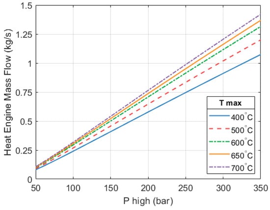
Figure 13. Mass flow through the heat engine to achieve an 80% isentropic expansion efficiency with a rotational speed limit of 170 k RPM.

We can see in Figure 13 that the heat engine’s mass flow increases as the expander’s inlet pressure and temperature increase. We can also see that inlet pressure has a greater effect on mass flow than inlet temperature.

In Section 4, a system sized for domestic applications with a thermal output of 10 kW was used as an example. In that system, with a $P_{high}$ of 250 bar and a $T_{max}$ of 650 °C, the mass flow of the heat engine part was about 5.4 × 10⁻³ kg/s. To achieve a good isentropic efficiency, the expanders of that system would need to be rotating at very high speeds. Here we can see that, as the rotational speed has been limited, the mass flow is much higher (~0.951 kg/s) for the same inlet conditions. This translates into a system with a greater thermal output.

The heat engine becomes more efficient as the inlet pressure and temperature of the expanders increase. The net work output of the heat engine increases with $P_{high}$ and $T_{max}$ due to the combined effect of (i) a greater mass flow and (ii) a higher efficiency. This allows the compressor of the heat pump to consume more work (by increasing mass flow), which in turn increases the heat output of the heat pump and of the overall HP³ system.

Figure 14 shows how the ratio of the heat engine mass flow relative to the mass flow through the heat pump changes with respect to the design parameters. Both mass flows increase as $P_{high}$ and $T_{max}$ increase; however, the mass flow on the heat pump side increases at a faster rate. The proportion shown here is the same as what was previously shown in Figure 9.

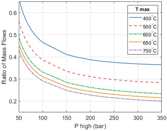
Figure 14. Relationship between the mass flows in the two parts of the system (Heat engine/Heat pump).

It has been established that the mass flow in the heat engine increases as $P_{high}$ and $T_{max}$ rise. In turn, this increases the thermal output of the heat engine, as Figure 15 shows.

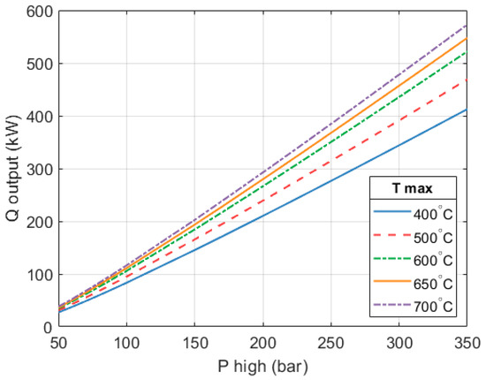
Figure 15. Thermal output of the heat engine part. Mass flow varies to maintain an expansion efficiency of 80% with a 170 k RPM rotational speed.

As mentioned, the heat engine’s shaft work increases as the expander’s inlet temperature and pressure increase. The mass flow on the heat pump side increases to push up the compressor work and consume the net work output of the heat engine. Consequently, the heat output of the heat pump also increases. Figure 16 shows how the total heat output of the full HP³ system varies as a function of the high-grade heat input temperature ($T_{max}$) and maximum system pressure ($P_{high}$).

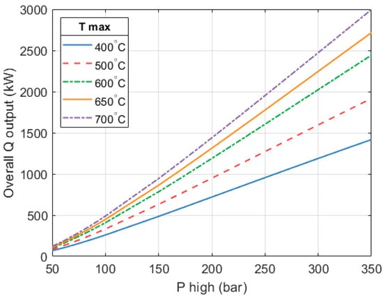
Figure 16. Overall heat output of the HP³ system. Expanders operate at constant efficiency of 80% and constant rotational speed (170 k RPM). Mass flow in the heat engine is variable.

The contribution of the heat pump part to the system’s total heat output (as a function of $P_{high}$ and $T_{max}$) is the same as what was previously presented in Figure 10. This is because the conditions of the working fluid (P, T, S, and H) at the different points throughout the system are not changing. In this revised calculation, where a rotational speed limit has been introduced, the only parameters that are changing are the mass flows in the two parts of the system.

With the chosen design parameters of 250 bar and 650 °C, the heat pump part provides 79.3% of the total heat output, while the remaining 20.7% comes from the heat engine.

The CoP_HP3 of the full HP³ system is still described by the surface previously shown in Figure 6. However, a summary of said surface is provided in Figure 17 for clarity.

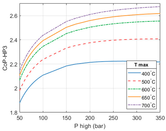
Figure 17. CoP_HP3 of the full HP³ system. Ambient temperature is −9 °C, condensing temperature is 40 °C and the expander efficiency is 80%.

In the selected configuration ($P_{high}$ = 250 bar and $T_{max}$ = 650 °C), a full system CoP_HP3 of 2.59 is achieved. An HP³ based on these design parameters will have a thermal output of 1.77 MW in order to achieve the desired isentropic expansion efficiency, which is key to maintaining a high overall CoP_HP3. Figure 18 shows how the CoP_HP3 of the system changes with ambient temperature. A $T_{max}$ of 650 °C is considered.

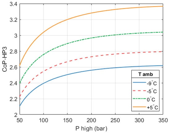
Figure 18. Effect of ambient temperature (low-grade source) on the CoP_HP3 of the full HP³ system. $T_{max}$ = 650 °C. Condensing temperature is 40 °C and the expander efficiency is 80%.

A thermal output of 1.77 MW is sufficient to provide space heating to between 180 and 220 dwellings in the UK. A higher CoP_HP3 could be achieved by using higher values of $P_{high}$ and $T_{max}$; however, the system output will also increase, and there are additional safety considerations.

The results presented in this section indicate that the HP³ concept is much better suited for larger-scale applications such as district heating or use in commercial buildings (e.g., hotels, shopping centers) rather than for residential-scale heating.

Hot water temperatures in district heating networks vary significantly by generation. Modern, fourth-generation district heating networks operate at lower temperatures, typically 50–60 °C flow and around 35 °C return [73]. HP³ systems can be seamlessly integrated with these temperature levels, requiring no modifications to the rest of the distribution system. The only interaction between an HP³ unit and the rest of the district system is the heat output unit (i.e., the condenser) which produces hot water. The temperature output of an HP³ system can be increased so it is compatible with older-generation district networks requiring higher temperatures; however, this comes with a penalty in terms of the CoP_HP3 (see Figure 4 and Figure 5).

As a summary, Table 3 provides the conditions of the working fluid (propane) at the different points in the system. The values shown in Table 3 correspond to the selected configuration (650 °C and 250 bar). Figure 19 shows the operation of this system’s configuration via a temperature-entropy diagram. Table 4 summarizes the system parameters of the selected “best” configuration, including heat and work flows across the two sections of the system.

Table 3. Operating conditions of the working fluid (R290) at different points in the system.

Point	Temp (°C)	Pressure (bar)	Enthalpy (kJ/kg)	Entropy (kJ/kgK)
1	−14	3	559.2	2.39
2	55.6	13.7	648.5	2.45
3	40	13.7	307.1	1.36
4	−14.2	3	294.9	1.37
5	60.5	250	367.4	1.40
6	523.1	250	1889.5	4.19
7	650	250	2375.7	4.76
8	587.8	58.5	2176.1	4.82
9	650	58.5	2410.9	5.08
10	594.7	13.7	2215.7	5.14
11	76.6	13.7	693.6	2.58

Figure 19. Temperature–entropy diagrams for the two sections of an HP³ system. (A) Heat pump and (B) heat engine. The diagrams show the preferred configuration, $T_{max}$ = 650 °C and $P_{high}$ = 250 bar. The numbers in the figures refer to the state points or nodes shown in Figure 3 and summarized in Table 3.

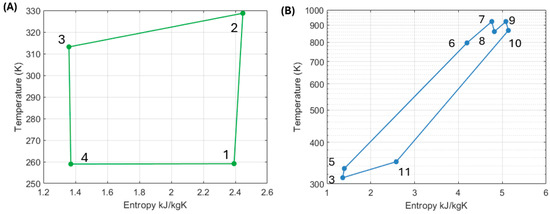
Table 4. Summary of system parameters for the selected HP³ configuration. Ambient temperature of −9 °C is considered as well as expander efficiencies of 80%.

	Parameter	Value
Heat Pump Section	Heat input	1090.79 kW
	Heat output	1408.87 kW
	Compressor work	368.68 kW
	Expander work	50.60 kW
	Net-work needed	318.08 kW
	Mass flow	4.13 kg/s
	CoP	4.43
Heat Engine Section	Heat input	685.64 kW
	Heat output	367.57 kW
	Expander work	375.40 kW
	Pump work	57.32 kW
	Net-work produced	318.08 kW
	Mass flow	0.95 kg/s
	Efficiency	46.39%
	Back work ratio	15.27%
Full HP3 System	Total high-grade heat input	685.64 kW
	Total low-grade heat input	1090.79 kW
	Total heat output	1776.44 kW
	Fraction of output provided by heat pump	79.31%
	Ratio of mass flows	4.34
	Full system CoPHP3	2.59

6. A “More Heat Engine” Design

This section briefly discusses how the CoP_HP3 of a complete HP³ system will vary if the system is allowed to be ‘more heat engine’ and produce some electricity on top of its nominal heat output.

In previous sections, the net work produced by the heat engine section was the same as the work consumed by the heat pump section. This represents a ‘balanced’ system. Here, the net work output of the heat engine part is defined as the sum of the work needed to drive the heat pump plus an additional amount ($E_{output}$) that will be used to drive an electrical generator, as shown in Equation (39):

$$E_{output}=Total Heat Output\times {\epsilon }_{fraction}$$

(38)

$$W_{net\text{-}engine}= W_{net heat pump }+E_{output}$$

(39)

The amount of electricity produced is expressed as a fraction of the system’s total heat output. For example, an HP³ system with a 10-kW heat output and an $\epsilon$ = 0.2 will produce 10 kW of low-grade heat for space heating and 2 kW of electricity.

For a system with a given nominal heat output, an increase in the electricity fraction ($\epsilon$) leads to an increase in the mass flow across the heat engine section. This is so that the heat engine can produce the additional work that will drive the electrical generator. In turn, this translates into a greater heat output from the heat engine, which causes the mass flow across the heat pump section to decrease so that the total heat output of the system remains at the specified level.

Figure 20 shows how the contribution of the heat pump part to the total heat output of the system decreases as the electricity output increases.

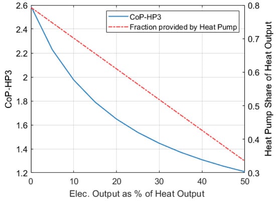
Figure 20. CoP_HP3 of an HP³ system with respect to its electricity output. Figure considers an ambient temperature of −9 °C, condensation temperature of 40 °C, $T_{max}$ = 650 °C and $P_{high}$ = 250 bar.

As previously mentioned, maximizing the contribution of the heat pump is desirable as it leads to a higher overall CoP_HP3. Figure 20 also shows how the CoP_HP3 of the full system decreases as the electricity output increases. In this case, the CoP_HP3 of the full system is calculated as indicated by Equation (40).

$$Co{P}_{HP3}={\displaystyle \frac{Total Heat Output+Elec Output}{Heat Engine Heat Input}}$$

(40)

When no electricity is produced ($\epsilon$ = 0), a CoP_HP3 of 2.59 is achieved. This scenario has been discussed in previous sections and considers an ambient temperature of −9 °C, a $T_{max}$ of 650 °C and a $P_{high}$ of 250 bar. If the system is allowed to generate an additional 10% of its heat output in the form of electricity, the CoP_HP3 will reduce to 1.975. If the electricity fraction ($\epsilon$) increases to 50%, then the CoP_HP3 will drop to 1.2.

The authors have explore how supplying a fraction of the country’s space heating demand with HP³ systems with varying electricity outputs can help to reduce the requirement for grid-scale energy storage compared to a scenario where electrical heat pumps are installed in 100% of UK homes [74].

7. Future Work

The study currently relies entirely on modeling. As a first step towards demonstrating the concept, we plan to develop a lab-scale proof of principle comprising a swimming pool heat pump (5.6 kW) coupled to a small petrol generator. The coupling will be electrical rather than mechanical, avoiding challenges such as speed control and torque matching. In this setup, the heat pump will deliver hot water that will be further heated in a heat exchanger by the generator’s exhaust gases. Although simple, this demonstrator will help us to validate aspects of the model and introduce additional realism by accounting for pressure drops, losses to the environment, auxiliary loads and other practical effects.

A central component of an HP³ system is the expander–compressor set. Our research group is partnering with two UK SMEs specializing in micro gas turbines to pursue additional innovation funding and develop a prototype of a mechanical compander for the HP³ system. While the prototype may not achieve the $P_{high}$ and $T_{max}$ considered in this study, thus reducing the achievable CoP_HP3, it will use propane as the working fluid, and it will enable further model validation, technology demonstration, and identification of design-improvement opportunities.

8. Concluding Remarks

A novel zero-carbon heating technology called “High-Performance Heat-Powered Heat Pumps” (HP³) has been discussed. The concept combines the best attributes of electrical heat pumps and hydrogen boilers while simultaneously removing some of their drawbacks. HP³ systems allow continued use of the existing gas infrastructure, offer much higher efficiencies than hydrogen boilers and avoid overwhelming the electricity grid. An HP³ system combines a heat pump with a heat engine. Unlike gas-engine-driven heat pumps (GEHP) where the coupling between the two parts is limited to a mechanical shaft, an HP³ system seeks a much tighter integration by using a common working fluid for both parts and a common heat output device (i.e., a condenser).

The paper provides a comprehensive discussion on the effect that different design variables have on the overall performance of an HP³ system.

The heat pump part is designed for an ambient temperature of −9 °C. A maximum CoP of the heat pump part of 4.43 is achieved with an evaporator pressure of 3 bar and a condenser pressure of 13.7 bar, which matches the saturation pressure of the working fluid (propane) at the respective temperatures.

The heat engine part absorbs high-grade heat from the combustion of hydrogen (or another clean fuel) and drives the compressor of the heat pump. A parametric exploration of the heat engine was carried out based on two variables: $P_{high}$ and $T_{max}$, representing the inlet pressure and temperature of the expansion train. The CoP of the full system (CoP_HP3) increases as these two parameters increase because the heat engine produces more work per unit of heat consumed and there is less heat rejected at the condenser. In turn, this allows the heat pump to contribute more to the total heat output of the HP³ system, benefiting the overall CoP_HP3.

A design based on a $P_{high}$ of 250 bar and a $T_{max}$ of 650 °C was selected as the ‘best’ design. These values are deemed a good compromise between performance, complexity, cost, and safety. With these parameters a full system CoP_HP3 of 2.59 is achieved. If ambient temperature were 5 °C instead of −9 °C, then the full system CoP_HP3 would increase to 3.32. Comparable GEHPs achieve CoPs between 1.5 and 1.8 at significantly higher ambient temperatures.

The paper presents a model to calculate expansion efficiency based on rotational speed and inlet conditions. A target expansion efficiency of 80% was defined and a limit of 170,000 RPM was set, which is comparable to the operating speeds of automotive turbochargers. A significant mass flow is required to achieve the target expansion efficiency with the rotational speed and inlet parameters (250 bar and 650 °C) specified. This leads to an overall heat output for the full HP₃ system of 1.77 MW, enough to provide space heating to between 180 and 220 UK dwellings. Reducing the thermal output requires reducing the mass flow, which in turn requires increasing the rotational speed. For example, a 10 kW system would need rotational speeds higher than 1 × 10⁶ RPM, far too high for a domestic-scale system.

Results from the modeling work reveal that the HP³ concept is much better suited for larger applications such as district heating systems rather than domestic-scale systems. The flow/return temperatures of the HP³ system are compatible with modern, 4th-generation district heating systems and the integration requires minimal to no changes to existing designs.

References

- Nesta. A Gas Boiler Emits More Annual CO2 Than Seven Transatlantic Flights. 2022. Available online: https://www.nesta.org.uk/press-release/gas-boiler-emits-more-annual-co2-seven-transatlantic-flights/ (accessed on 1 December 2025).
- UK Department for Energy Security and Net Zero. National Audit Office. Decarbonising Home Heating. 2024. Available online: https://www.nao.org.uk/wp-content/uploads/2024/03/Decarbonising-home-heating-HC-581-SUMMARY.pdf (accessed on 17 September 2025).
- UK Department for Business, Energy and Industrial Strategy. Building for 2050: Low Cost, Low Carbon Homes. 2022. Available online: https://www.gov.uk/government/publications/building-for-2050/building-for-2050-low-cost-low-carbon-homes (accessed on 1 December 2025).
- Energy Systems Catapult. A Guide to the Decarbonisation of Heat in the UK. 2025. Available online: https://es.catapult.org.uk/guide/decarbonisation-heat/ (accessed on 17 September 2025).
- Hydrogen UK. Recommendations for the Acceleration of Hydrogen Networks. 2023. Available online: https://hydrogen-uk.org/wp-content/uploads/2023/02/HUK_Recommendations-for-the-Acceleration-of-Hydrogen-Networks_online-Jan23.pdf (accessed on 17 September 2025).
- Sargent, M.; Sargent, P. Moving hydrogen through the UK gas distribution network. Int. J. Hydrogen Energy 2024, 87, 1–9. [Google Scholar] [CrossRef]
- UK Department for Energy Security and Net Zero. Official Statistics: Subnational Estimates of Properties Not Connected to the Gas Network 2015–2023. Available online: https://www.gov.uk/government/statistics/sub-national-estimates-of-households-not-connected-to-the-gas-network (accessed on 17 September 2025).
- National Gas. Future Grid. 2025. Available online: https://www.nationalgas.com/future-energy/futuregrid (accessed on 17 September 2025).
- National Gas. Project Union. 2025. Available online: https://www.nationalgas.com/future-energy/hydrogen/project-union (accessed on 17 September 2025).
- Steward, D. National Gas. Project Union. Presented at the Energy Innovation Summit 2023. Available online: https://smarter.energynetworks.org/media/sblno3qy/1400-1530_31-october-2023_hydrogen-horizons-harnessing-the-power-of-an-alternative-gas_stewart.pdf (accessed on 17 September 2025).
- Energy Networks Association. Northern Gas Networks: H21. 2025. Available online: https://smarter.energynetworks.org/projects/ngngn04/ (accessed on 17 September 2025).
- Northern Gas Networks. H21 North of England Report. 2018. Available online: https://www.northerngasnetworks.co.uk/wp-content/uploads/2024/09/H21-NoE-Exec-Sum-Print-Final.pdf (accessed on 17 September 2025).
- SGN. A World-First Green Hydrogen Gas Network in the Heart of Fife. 2025. Available online: https://www.h100fife.co.uk/ (accessed on 17 September 2025).
- Pipeline Technology Journal. The LTS Futures Project. 2024. Available online: https://www.pipeline-journal.net/articles/lts-futures-project-uk-operators-sgn-experience-assessing-feasibility-repurposing-their (accessed on 17 September 2025).
- Armitage, T. Underground Hydrogen Storage: Insights and Actions to Support the Energy Transition. British Geological Survey. 2025. Available online: https://www.bgs.ac.uk/download/science-briefing-note-underground-hydrogen-storage-insights-and-actions-to-support-the-energy-transition/ (accessed on 17 September 2025).
- Khavari, F.; Hajipour, E.; Liu, J. Energy management considering underground hydrogen storage. J. Energy Storage 2025, 127, 116946. [Google Scholar] [CrossRef]
- Feng, C.; Jing, Z.; Kang, Y.; Gao, Y.; Wang, X. Influences of operational parameters on the feasibility and performance of underground hydrogen storage: A review. J. Energy Storage 2026, 142, 119666. [Google Scholar] [CrossRef]
- Thiyagarajan, S.R.; Emadi, H.; Hussain, A.; Patange, P.; Watson, M. A comprehensive review of the mechanisms and efficiency of underground hydrogen storage. J. Energy Storage 2022, 51, 104490. [Google Scholar] [CrossRef]
- Kumar, K.R.; Honorio, H.; Chandra, D.; Lesueur, M.; Hajibeygi, H. Comprehensive review of geomechanics of underground hydrogen storage in depleted reservoirs and salt caverns. J. Energy Storage 2023, 73, 108912. [Google Scholar] [CrossRef]
- Chen, Y.; Hill, D.; Billings, B.; Hedengren, J.; Powell, K. Hydrogen underground storage for grid electricity storage: An optimization study on techno-economic analysis. Energy Convers. Manag. 2024, 322, 119115. [Google Scholar] [CrossRef]
- Yuan, C.; Yu, X.; Li, P.; Shan, X.; Hong, W.; Li, Y.; Chen, Z.; Liu, C.; Wu, K. From micro to macro: A comprehensive review for underground hydrogen storage technologies and challenges. Renew. Sustain. Energy Rev. 2025, 224, 116090. [Google Scholar] [CrossRef]
- Zheng, L.; Jing, Z.; Feng, C.; Wang, L.; Zhou, Y.; Qiao, M.; Liu, Z. Underground hydrogen storage (UHS): Comparative analysis of key performance metrics. Renew. Sustain. Energy Rev. 2026, 226, 116446. [Google Scholar] [CrossRef]
- Brading, B. Natural Gas Storage in the UK. Business Energy Deals. Available online: https://www.businessenergydeals.co.uk/blog/natural-gas-storage/ (accessed on 17 September 2025).
- Nikše, D. Centrica Cleared to Operate ‘UK’s Largest Gas Storage Facility’ for Another Year. Offshore Energy. 2025. Available online: https://www.offshore-energy.biz/centrica-cleared-to-operate-uks-largest-gas-storage-facility-for-another-year/ (accessed on 17 September 2025).
- Cebon, D. Hydrogen for Heating? A Comparison with Heat Pumps (Part 1). 2022. Hydrogen Science Coalition. Available online: https://h2sciencecoalition.com/blog/hydrogen-for-heating-a-comparison-with-heat-pumps-part-1/ (accessed on 17 September 2025).
- Harris, B.; Walker, A. Research Briefing: Heat Pumps. UK Parliamentary Office of Science and Technology. 2023. Available online: https://post.parliament.uk/research-briefings/post-pn-0699/ (accessed on 17 September 2025).
- Wilson, G.; Taylor, R.; Rowley, P. Challenges for the Decarbonisation of Heat: Local gas Demand vs Electricity Supply Winter 2017/2018. UK Energy Research Centre. 2018. Available online: https://ukerc.ac.uk/publications/local-gas-demand-vs-electricity-supply/ (accessed on 17 September 2025).
- Gridwatch. GB National Grid Status. Available online: https://www.gridwatch.templar.co.uk/ (accessed on 17 September 2025).
- Elexon. Balancing and Settlement Code. Actual Aggregated Generation per Type. Available online: https://bmrs.elexon.co.uk/actual-aggregated-generation-per-type (accessed on 17 September 2025).
- Few, J.; Pullinger, M.; McKenna, E.; Elam, S.; Ashdown, M.; Hanmer, C.; Zapata-Webborn, E.; Oreszczyn, T. Smart Energy Research Lab: Energy Use in GB Domestic Buildings 2022 and 2023; Smart Energy Research Lab: London, UK, 2024. [Google Scholar]
- Chesser, M.; Lyons, P.; O’Reilly, P.; Carroll, P. Air source heat pump in-situ performance. Energy Build. 2021, 251, 111365. [Google Scholar] [CrossRef]
- Li, H.; Xu, Z.; Yang, Q.; Wang, Z.; Shao, S.; Xu, C.; Yang, Y.; Li, J. Efficiency assessment of variable speed air source heat pump heating systems: A hybrid data-driven and theoretical approach. J. Build. Eng. 2024, 87, 109018. [Google Scholar] [CrossRef]
- Energy Systems Catapult. Electrification of Heat Demonstration Project: Insights from Heat Pump Performance Data. 2024. Available online: https://es.catapult.org.uk/project/electrification-of-heat-demonstration-project/ (accessed on 1 December 2025).
- Lämmle, M.; Bongs, C.; Wapler, J.; Günther, D.; Hess, S. Performance of air and ground source heat pumps retrofitted to radiator heating systems and measures to reduce space heating temperatures in existing buildings. Energy 2022, 242, 122952. [Google Scholar] [CrossRef]
- Zhang, M.; Millar, M.A.; Yu, Z.; Yu, J. An assessment of the impacts of heat electrification on the electric grid in the UK. Energy Rep. 2022, 8, 14934–14946. [Google Scholar] [CrossRef]
- University of Oxford-Department of Engineering Science. How Heat Pumps Can Keep Homes Warm Without Frying the Power Grid. 2023. Available online: https://eng.ox.ac.uk/news/how-heat-pumps-can-keep-homes-warm-without-frying-the-power-grid/ (accessed on 17 September 2025).
- Watson, S.D.; Crawley, J.; Lomas, K.J.; Buswell, R.A. Predicting future GB heat pump electricity demand. Energy Build. 2023, 286, 112917. [Google Scholar] [CrossRef]
- Whalen, C. How Much Electricity Will the UK Need as it Switches to Electric Heating and Cars? Carbon Commentary. 2022. Available online: https://www.carboncommentary.com/blog/2022/2/11/how-much-electricity-will-the-uk-need-as-it-switches-to-electric-heating-and-cars (accessed on 17 September 2025).
- Turner, P.A.D.; Rushby, T.W.; Manfren, M.; James, P.A.B.; Gauthier, S.; Bahaj, A.S.; Sweetnam, T.; Kim, S.; Ridett, E. Embedding energy flexibility capability in air source heat pumps via third-party control: Insights from a field trial on residential buildings in England. Appl. Energy 2025, 389, 125705. [Google Scholar] [CrossRef]
- Cárdenas, B.; Garvey, S.; Mehdipour, Z.B.R. Heat Pumps and the Requirement for Grid-Scale Energy Storage in the UK. IET Conf. Proc. 2025, 2024, 14–19. [Google Scholar] [CrossRef]
- Cárdenas, B.; Garvey, S.; Baniamerian, Z.; Mehdipour, R. Heat pumps’ impact on the requirement for grid-scale energy storage in the UK. Renew. Energy 2025, 247, 123020. [Google Scholar] [CrossRef]
- National Energy System Operator. Beyond 2030: A National Blueprint for a Decarbonised Electricity System in Great Britain. 2024. Available online: https://www.neso.energy/document/304756/download (accessed on 17 September 2025).
- Hodgson, F. Building a GB Electricity Network Ready for Net Zero. Regen. 2023. Available online: https://www.regen.co.uk/insights/prepare-britains-electricity-network-for-net-zero (accessed on 21 September 2025).
- Grid Can Cope with Increased Electrification. 2023. Available online: https://www.installeronline.co.uk/green-energy/grid-can-cope-with-increased-electrification-says-new-report/ (accessed on 21 September 2025).
- Chen, X.; Li, S.; Feng, Z.; Song, W.; Shu, J.; Ma, Z.; Hao, C. Partial-load operation characteristics of air-source gas engine-driven heat pump system in heating mode. Int. J. Refrig. 2026, 181, 306–316. [Google Scholar] [CrossRef]
- Hu, Y.; Feng, Z.; Song, W. Study on performance of a gas engine-driven heat pump system with R410A for heating and domestic hot water applications. Appl. Therm. Eng. 2023, 228, 120538. [Google Scholar] [CrossRef]
- Hu, Y.; Lv, J.; Huang, C.; Song, W.; Feng, Z. Experimental investigation on heating performance of a gas engine-driven heat pump system with R410A. Appl. Therm. Eng. 2022, 215, 118863. [Google Scholar] [CrossRef]
- Pawela, B.; Jaszczur, M. Review of gas engine heat pumps. Energies 2022, 15, 4874. [Google Scholar] [CrossRef]
- Hocking, M.B. Petrochemicals. In Handbook of Chemical Technology and Pollution Control, 3rd ed.; Academic Press: Cambridge, MA, USA, 2005; Chapter 19; pp. 637–668. [Google Scholar]
- Kawai, K.; Yoshikawa, K.; Kobayashi, H.; Tsai, J.S.; Matsuo, M.; Katsushima, H. High temperature air combustion boiler for low BTU gas. Energy Convers. Manag. 2002, 43, 1563–1570. [Google Scholar] [CrossRef]
- Gong, Y.; Ma, G.; Jiang, Y.; Wang, L. Research progress on the fifth-generation district heating system based on heat pump technology. J. Build. Eng. 2023, 71, 106533. [Google Scholar] [CrossRef]
- Dang, L.M.; Nguyen, L.Q.; Nam, J.; Nguyen, T.; Lee, S.; Song, H.K.; Moon, H. Fifth generation district heating and cooling: A comprehensive survey. Energy Rep. 2024, 11, 1723–1741. [Google Scholar] [CrossRef]
- UK Committee on Climate Change. The Seventh Carbon Budget: Advice for the UK Government. 2025. Available online: https://www.theccc.org.uk/publication/the-seventh-carbon-budget/ (accessed on 1 December 2025).
- Ofgem. Average Gas and Electricity Usage. 2025. Available online: https://www.ofgem.gov.uk/information-consumers/energy-advice-households/average-gas-and-electricity-use-explained (accessed on 1 December 2025).
- Carbon Independent. Emissions from Home Energy Use. 2025. Available online: https://www.carbonindependent.org/15.html (accessed on 1 December 2025).
- US Energy Information Administration. Carbon Dioxide Emissions Coefficients. 2024. Available online: https://www.eia.gov/environment/emissions/co2_vol_mass.php (accessed on 1 December 2025).
- American Geosciences Institute. How Much Carbon Dioxide is Produced When Different Fuels are Burned? 2025. Available online: https://profession.americangeosciences.org/society/intersections/faq/how-much-carbon-dioxide-produced-when-different-fuels-are-burned/ (accessed on 1 December 2025).
- US Energy Information Administration. How Much Carbon Dioxide is Produced per Kilowatt-Hour of U.S. Electricity Generation? 2023. Available online: https://www.eia.gov/tools/faqs/faq.php?id=74&t=11 (accessed on 1 December 2025).
- Roy, R.; Antonini, G.; Hayibo, K.S.; Rahman, M.; Khan, S.; Tian, W.; Boutilier, M.S.H.; Zhang, W.; Zheng, Y.; Bassi, A.; et al. Comparative techno-environmental analysis of grey, blue, green/yellow and pale-blue hydrogen production. Int. J. Hydrogen Energy 2025, 116, 200–210. [Google Scholar] [CrossRef]
- Hammi, Z.; Labjar, N.; Dalimi, M.; El Hamdouni, Y.; Lotfi, E.M.; El Hajjaji, S. Green hydrogen: A holistic review covering life cycle assessment, environmental impacts, and color analysis. Int. J. Hydrogen Energy 2024, 80, 1030–1045. [Google Scholar] [CrossRef]
- Dorn, F.M. Towards a multi-color hydrogen production network? Competing imaginaries of development in northern Patagonia, Argentina. Energy Res. Social Sci. 2024, 110, 103457. [Google Scholar] [CrossRef]
- Heat Pump Association. Types of Heat Pump. Available online: https://www.heatpumps.org.uk/types-of-heat-pump/ (accessed on 29 September 2025).
- Lemmon, E.W.; Bell, I.H.; Huber, M.L.; McLinden, M.O. NIST Standard Reference Database 23: Reference Fluid Thermodynamic and Transport Properties-REFPROP, Version 10.0; National Institute of Standards and Technology-Standard Reference Data Program: Gaithersburg, MD, USA, 2018. [Google Scholar]
- Lemmon, E.W.; McLinden, M.O.; Wagner, W. Thermodynamic Properties of Propane. III. A Reference Equation of State for Temperatures from the Melting Line to 650 K and Pressures up to 1000 MPa. J. Chem. Eng. Data 2009, 54, 3141–3180. [Google Scholar] [CrossRef]
- Kang, J.; Ran, J.; Niu, J.; Shi, J.; He, J.; Yang, Z. Experimental and theoretical study on propane pyrolysis to produce gas and soot. Int. J. Hydrogen Energy 2019, 44, 22904–22918. [Google Scholar] [CrossRef]
- Lifshitz, A.; Frenklach, M. Mechanism of the high temperature decomposition of propane. J. Phys. Chem. 1975, 79, 686–692. [Google Scholar] [CrossRef]
- American Society of Mechanical Engineers. Section II: Materials, Part D—Properties (Table 1A: Maximum Allowable Stress Values for Ferrous Materials). In ASME Boiler and Pressure Vessel Code; ASME: New York, NY, USA, 2010; pp. 86–89. [Google Scholar]
- Thunder Said Energy. Gas Turbines: Operating Parameters? 2025. Available online: https://thundersaidenergy.com/downloads/gas-turbines-operating-parameters/ (accessed on 1 December 2025).
- AET Turbos. How a Turbo Works Details and Principles of Design. Available online: https://aet-turbos.co.uk/principles-of-design/ (accessed on 29 September 2025).
- Turbo Dynamics. Turbocharger Diagnostics. Available online: https://www.turbodynamics.co.uk/diagnostics (accessed on 29 September 2025).
- Goldfarb, S. How Long Do Turbos Last? 2023. Available online: https://goldfarbinc.com/blogs/news/how-long-do-turbos-last (accessed on 1 December 2025).
- TurboTurbos. Turbo longevity: How long do they really last? 2025. Available online: https://turboturbos.com/blogs/news/turbo-longevity-how-long-do-they-really-last (accessed on 1 December 2025).
- Jodeiri, A.M.; Goldsworthy, M.J.; Buffa, S.; Cozzini, M. Role of sustainable heat sources in transition towards fourth generation district heating–A review. Renew. Sustain. Energy Rev. 2022, 158, 112156. [Google Scholar] [CrossRef]
- Cardenas, B.; Garvey, S.D.; Baniamerian, Z.; Mehdipour, R. How heat-powered heat pumps could reduce the need for grid-scale energy storage. Energies 2025, 18, 5887. [Google Scholar] [CrossRef]
Disclaimer/Publisher’s Note: The statements, opinions and data contained in all publications are solely those of the individual author(s) and contributor(s) and not of MDPI and/or the editor(s). MDPI and/or the editor(s) disclaim responsibility for any injury to people or property resulting from any ideas, methods, instructions or products referred to in the content. |
© 2025 by the authors. Licensee MDPI, Basel, Switzerland. This article is an open access article distributed under the terms and conditions of the Creative Commons Attribution (CC BY) license.