Smart Hybrid Maintenance as a Pathway to Energy-Efficient Manufacturing

Abstract

The growing demand for energy-efficient and sustainable manufacturing requires maintenance strategies that extend beyond reliability optimization toward active energy management. This study proposes a Smart Hybrid Maintenance System (SHMS) that integrates Reliability-Centered Maintenance (RCM) and Condition-Based Maintenance (CBM) principles with energy performance assessment. The framework combines classical reliability indicators (MTBF, MTTR, and Availability) with energy-oriented Key Performance Indicators (EEI, EENS, and OEE) to quantify the relationship between machine degradation, operational availability, and energy efficiency. The methodology was validated using two datasets: NASA N-CMAPSS for simulation-based benchmarking and the Smart RDM industrial environment for real process data. Results demonstrate that predictive maintenance supported by the Hybrid Risk Index ($HRI$) reduces unplanned downtime by up to 12%, corresponding to a 7–9% decrease in specific energy consumption and a measurable improvement in the Energy Efficiency Index. By embedding energy metrics into predictive maintenance decision-making, the SHMS enables dual optimization of reliability and energy performance. The proposed approach not only enhances equipment availability and cost efficiency but also supports industrial decarbonization targets, positioning predictive maintenance as a key enabler of energy-aware and sustainable manufacturing aligned with Industry 5.0 objectives.

1. Introduction

1.1. Energy Efficiency as a Driver of Predictive Maintenance Strategies

In modern industry, energy efficiency has become a strategic factor linking operational performance, economic competitiveness, and environmental sustainability. The manufacturing and energy sectors account for a major share of global energy consumption, and even small improvements in efficiency translate into measurable reductions in operating costs and greenhouse gas emissions. Maintenance engineering plays a crucial yet often underestimated role in this context. Studies demonstrate that the degradation of technical systems, process instability, and unplanned downtime generate hidden energy losses that can reach 10–20% of total plant energy consumption [1,2]. Therefore, maintenance policies must increasingly account not only for reliability and cost but also for their impact on overall energy performance.

A pioneering study introduced the concept of integrating energy efficiency indicators into Condition-Based Maintenance (CBM) decision-making [1]. Using the Energy Efficiency Indicator (EEI)—the ratio between useful output and energy input—it was shown that maintenance actions triggered by a decline in energy efficiency can significantly reduce both energy losses and maintenance costs in manufacturing systems. This framework redefined maintenance from a purely reliability-driven activity into a key element of energy management.

Several studies extend this perspective by coupling predictive maintenance with machine learning and sustainability-oriented optimization [3]. Data-driven models can identify energy inefficiencies before they escalate, and modern Long Short-Term Memory (LSTM) architectures can predict component degradation and enable energy savings—by up to 9% in compressed air systems and over 12% in hot rolling mills—through improved control of radiator and motor operation cycles [4,5]. These examples confirm that energy-aware predictive maintenance is no longer theoretical but increasingly a practical tool for industrial optimization.

In the energy sector, condition-based and reliability-centered maintenance have proven to be particularly effective in reducing unplanned stoppages and associated energy waste [6]. Integrated CBM and RCM models for offshore wind turbines optimize maintenance schedules to minimize expected energy not supplied (EENS) and thereby increase total power output. A similar approach applied to steam boiler systems showed that optimized maintenance intervals based on reliability indicators reduced fuel consumption and improved overall thermal efficiency by nearly 6% [7]. These results highlight that predictive maintenance is not only about asset health but is also directly tied to energy productivity and emissions reduction.

Complementary research underscores the role of digitalization and data analytics in achieving energy savings through maintenance optimization [8]. Frameworks that integrate Big Data mapping with predictive models support maintenance decisions balancing performance and energy consumption. Likewise, holistic approaches to asset management that include energy performance as a lifecycle criterion for decision-making emphasize that sustainable maintenance requires considering both technical reliability and the energy footprint of assets throughout their operation [9].

Energy-driven maintenance optimization has also been explored through mathematical modeling. An energy consumption-based optimization approach allows for the selection of maintenance strategies that minimize total energy use and greenhouse gas emissions [10]. Aligning maintenance timing with low-energy operating periods can yield up to 38% savings in total energy-related costs, providing a strong quantitative foundation for incorporating energy efficiency into maintenance policy design.

At the component and system monitoring level, recent advances in IoT and AI enhance energy-aware diagnostics [11]. Explainable deep learning frameworks for predictive maintenance of air compressors are capable of linking degradation patterns to energy performance in real time, achieving both improved model transparency and measurable energy savings. Similarly, IoT-based energy-efficient CBM frameworks for Industry 4.0 applications demonstrate that integrating energy-related features into predictive models can reduce overall energy waste while maintaining equipment reliability [12].

The importance of such strategies is further reinforced by reviews of diagnostic methods for electrical equipment, which conclude that predictive analytics and condition monitoring significantly contribute to energy-efficient system operation by reducing unplanned downtime and extending equipment lifecycles [2].

Taken together, these studies converge on the conclusion that predictive and condition-based maintenance are not only reliability management tools but also crucial enablers of energy efficiency and sustainability. By leveraging data analytics, IoT sensing, and machine learning, PdM systems can detect degradation early, optimize energy use, and synchronize maintenance with production and demand profiles.

In the context of this work, we extend these principles by developing a hybrid predictive maintenance framework that integrates reliability-centered maintenance with energy performance indicators to enhance both equipment availability and energy efficiency. This approach aligns with the broader objective of smart industrial systems—maximizing operational performance while minimizing energy intensity and environmental impact.

The integration of predictive maintenance with energy management principles has therefore become a natural progression in industrial optimization strategies. While Section 1.1 established energy efficiency as a key driver of maintenance transformation, the following part elaborates on how predictive maintenance (PdM) methods directly contribute to achieving this objective through data analytics, reliability modeling, and process automation.

Specifically, this work contributes to (i) an energy-aware hybrid PdM framework (RCM + CBM) operationalized via the Hybrid Risk Index, (ii) a methodology to quantify energy impacts through EEI/EENS/OEE linkages, and (iii) a comparative evaluation on benchmark and industrial datasets highlighting measurable availability and energy-performance gains.

1.2. Predictive Maintenance as a Tool for Energy Optimization

Predictive Maintenance (PdM) has emerged as a transformative paradigm in modern industrial operations, fundamentally reshaping how organizations approach equipment reliability and operational efficiency. In an increasingly competitive global manufacturing landscape, industries face constant pressure to maximize productivity, minimize downtime, and reduce operational expenditures. This has accelerated the transition from reactive to proactive maintenance strategies, driven by advances in the Industrial Internet of Things (IIoT), big data analytics, and artificial intelligence (AI) [13]. The application of PdM extends across numerous industrial sectors, including manufacturing, energy, transportation, and healthcare. The core tasks of predictive models include the prediction of failure events, estimation of the Remaining Useful Life (RUL) of critical components, and the enhancement of production performance through downtime reduction. These objectives are accompanied by challenges such as data heterogeneity, the need for sophisticated data models, difficulties in result interpretation, and scalability limitations. Addressing these challenges requires the integration of digital twins and machine learning algorithms with physical reliability models [14].

PdM represents a maintenance strategy based on continuous monitoring of the actual technical condition of equipment and forecasting failures before breakdowns occur. In contrast to Preventive Maintenance (PM), PdM is inherently data-driven, relying on sensors, analytical models, and machine learning [13]. Such data are used to forecast when a failure is likely to happen, allowing maintenance to be performed only when truly necessary [15]. This approach reduces both maintenance costs and downtime, while improving resource utilization and extending asset lifespan. However, the implementation of PdM requires the development of advanced data infrastructure and monitoring systems, making it more complex and resource-intensive to deploy.

It should be noted that PdM and PM are closely interrelated—not as competing, but as complementary approaches within an integrated maintenance strategy. PdM adds an analytical and predictive layer to maintenance operations. Frequently, data collected as part of PM programs, such as failure histories or inspection cycles, are utilized in predictive models for downtime forecasting. Therefore, PdM can be considered the next evolutionary step in enterprise maintenance maturity. In practice, deploying such advanced methods is feasible only when a sufficient and reliable dataset is available [16].

A key aspect of PdM is the prediction of failures and the planning of maintenance activities based on actual asset condition data, rather than on rigid time-based schedules. To achieve this, a structured sequence of steps is typically employed, encompassing data acquisition, analysis, and interpretation. In particular, the following stages can be distinguished [16,17]:

• Identification of critical assets;
• Data acquisition;
• Development of a consistent data model;
• Data flow design and storage architecture;
• Data preprocessing;
• Implementation of predictive algorithms and model training;
• Evaluation of PdM process performance through KPI calculation;
• Visualization and interpretation of results;
• Decision-making and execution of maintenance actions;
• Continuous process improvement.

Figure 1 presents a data flow diagram illustrating the implementation and operation of a PdM system. Each stage of the PdM deployment process is represented by a distinct block. Within each block, a specific activity is defined, together with the required data and resources necessary for the successful execution of subsequent steps.

Figure 1. Stages of PdM process deployment.

A properly functioning PdM system requires the execution of several data engineering tasks to prepare an appropriate dataset. In general, it is necessary to collect information concerning process parameters and associated events. This includes sensor measurement data, records of events and downtimes, as well as inspection and repair histories, which enable characterization of the lifecycle of individual machines or their components. Additionally, information on defined operational conditions—such as duty cycles, load levels, and nominal parameters—is essential. A well-prepared machine inventory, including machine types, categories, and operational times, is also a prerequisite.

Data requirements may vary depending on the applied methodology. For example, when Condition-Based Maintenance (CBM) is employed, process data are of primary importance. Machine learning models, in turn, can be enhanced with information about downtimes, failures, or other historical events. The development of a digital twin, on the other hand, requires design data necessary to construct a digital representation of a machine and subsequently feed it with historical operational data.

It should be emphasized that the use of a single data model may not yield satisfactory results. Therefore, it is recommended to combine various modeling approaches and develop a hybrid system. Recent research has demonstrated significant progress in the construction and application of health indicators (HIs) for predictive maintenance. Feature-level fusion methods combined with stochastic degradation modeling have been shown to improve RUL prediction accuracy and support cost-driven maintenance optimization, as exemplified by the KPCA–DAE framework proposed by Chen et al. [18]. In parallel, recent studies emphasize the integration of HIs within digital twin architectures, where HIs serve as key enablers of monitoring, diagnostics, and prognostics, enhancing system transparency and uncertainty awareness [19].

While these approaches significantly advance health assessment and prognostic capabilities, maintenance decisions are typically derived from RUL estimates, threshold-based rules, or external optimization layers. In contrast, the approach proposed in this work explicitly operates at the decision level. By integrating reliability-based survival analysis with condition-based anomaly assessment into a unified Hybrid Risk Index, and by introducing the Optimal Maintenance Point as a formally defined decision construct, the proposed framework directly links health assessment to maintenance action selection. This distinction enables the transition from descriptive and prognostic indicators toward an operational, risk-aware maintenance decision-making paradigm.

In this context, we introduce the Smart Hybrid Maintenance System (SHMS)—a comprehensive framework that integrates the principles of Reliability-Centered Maintenance (RCM) and CBM. RCM provides a structured methodology for identifying and managing critical assets based on their functions and failure consequences, while CBM leverages real-time sensor data and continuous monitoring to assess equipment condition [20]. The SHMS architecture enhances these traditional approaches by incorporating machine learning (ML) techniques, enabling predictive modeling based on both historical failure data and live operational inputs [21]. A schematic overview of the SHMS architecture is provided in Figure 2 (see also [22]).

Figure 2. Schematic representation of the Smart Hybrid Maintenance System (SHMS).

At the core of SHMS lies the Hybrid Risk Index ($HRI$), a composite Key Performance Indicator (KPI) that quantifies failure risk. The $HRI$ integrates two components: Failure Probability ($FP$), derived from statistical reliability models, and Anomaly Level ($AL$), calculated using AI/ML models detecting deviations from expected behavior. Time series data from condition monitoring (CBM) and maintenance management systems (RCM) are used to calculate $AL$ and $FP$, which are then combined into the $HRI$. The $HRI$ is normalized on a scale from 0 to 1, allowing for continuous monitoring of risk levels and informed maintenance decisions (Figure 3).

Figure 3. Conceptual representation of the Hybrid Risk Index ($HRI$) construction.

The computation of $HRI$ combines historical failure patterns, operating profiles, real-time condition monitoring data (e.g., temperature, vibration, current), predictive model outputs, and expert knowledge from maintenance personnel. This hybridized perspective ensures that both data-driven predictions and human expertise are incorporated into maintenance decision-making.

In practice, $HRI$ serves as a decision-support mechanism, enabling maintenance teams to assess equipment condition in both nominal and actual operational contexts. It supports timely intervention by identifying early signs of degradation, improving asset availability, and aligning maintenance activities with reliability policies.

Another key concept introduced within SHMS is the Optimal Maintenance Point ($OMP$), which defines the point in a system’s lifecycle where maintenance is most economically and operationally advantageous. It is characterized by a combination of increasing failure probability and a cost–benefit balance where the expense of preventive action is lower than the potential cost of downtime or failure.

Determining the $OMP$ requires operational experience, cost analysis, and understanding of equipment criticality in terms of production, quality, and safety. The $OMP$ supports a balanced approach—avoiding both premature maintenance (leading to unnecessary cost) and delayed action (resulting in failures and unplanned downtime). The bar plots in Figure 3 visualize $HRI$ levels with risk zones highlighted by pattern-filled regions.

SHMS is designed not as a black-box model but as an interpretable, context-aware solution reflecting the operational realities of a specific facility. It relies on predefined thresholds and rules derived from organizational standards and accumulated domain expertise. These setpoints convert sensor readings into actionable insights and trigger appropriate maintenance actions. The system incorporates operator input and expert feedback, fostering a human-centric maintenance paradigm where AI augments, rather than replaces, human decision-making.

The success of predictive maintenance initiatives such as SHMS depends strongly on the availability, quality, and contextual relevance of data. Historical records—failure logs, maintenance interventions—form the foundation for model training. Contextual data on load, environment, and utilization improve the interpretability of real-time signals [13,23]. Data deficiencies—such as incompleteness, noise, or poor integration—can impair model performance, leading to missed detections or false alarms [24]. Robust data acquisition and integration frameworks are therefore essential prerequisites for effective PdM.

Within this data-centric context, digital twins have emerged as powerful enablers of PdM. By creating high-fidelity virtual representations of physical assets, digital twins support real-time synchronization, scenario simulation, and advanced diagnostics, enhancing proactive maintenance and process optimization [24].

One of the most significant benefits of PdM is its impact on Overall Equipment Effectiveness (OEE)—a metric encompassing availability, performance, and quality dimensions. Originally introduced by Nakajima [25] within the Total Productive Maintenance (TPM) framework, OEE remains a cornerstone of performance measurement [26,27,28]. In the era of digital transformation, OEE serves as a baseline indicator for assessing progress and guiding maintenance investment priorities [29].

PdM directly improves OEE by minimizing unplanned downtime, optimizing resource utilization, and enhancing product quality [30]. It is often implemented in combination with Autonomous Maintenance (AM), where operators perform routine inspections and minor maintenance tasks. This decentralized approach increases responsiveness and ownership [25]. When effectively integrated, PdM and AM create a mutually reinforcing system that strengthens reliability and operational excellence [26].

To fully realize the potential of SHMS and PdM, organizations must prioritize digitalization—automating data collection, deploying integrated systems, and ensuring real-time process visibility [29]. Such digital infrastructure not only enables predictive and autonomous maintenance but also fosters continuous improvement, data-driven decision-making, and strategic alignment between operational and enterprise objectives.

In this paper, we present the SHMS framework, describing its theoretical foundation, data-driven architecture, and integration of domain expertise with operator knowledge. The SHMS is applied to a simulated real-world manufacturing environment, where the configuration of the $OMP$ is demonstrated based on historical data and operational scenarios. The effectiveness of the system is evaluated through a comparative study, analyzing operational outcomes between a machine equipped with SHMS and one without predictive maintenance functionality. This analysis demonstrates the practical advantages of SHMS in enhancing reliability, reducing costs, and improving overall operational performance. As predictive maintenance systems mature, their integration with reliability-centered approaches becomes essential to ensure both operational resilience and sustainable energy performance. The next section introduces the RCM framework, emphasizing its complementary role in aligning equipment reliability with the objectives of energy efficiency and optimized resource utilization.

1.3. Reliability-Centered Maintenance (RCM)

1.3.1. Introduction to RCM

RCM represents a sophisticated process through which organizations systematically identify and manage physical assets essential for their production processes with respect to reliability [31]. This comprehensive methodology enables organizations to develop and implement strategies that maintain equipment at optimal operational levels while balancing reliability requirements with resource constraints. The framework integrates multiple maintenance approaches, including Preventive Maintenance, Corrective Maintenance (also termed reactive maintenance), and Proactive Maintenance, to enhance the probability that equipment and components will function as required throughout their design lifecycle while minimizing maintenance requirements and downtime. These fundamental maintenance strategies are not implemented in isolation but rather integrated systematically to leverage their respective advantages, thereby maximizing facility and equipment reliability while optimizing lifecycle costs [32].

The fundamental principle of RCM is predicated on the optimization of maintenance decision-making processes to maximize equipment longevity while concurrently minimizing associated maintenance expenditures. The implementation of an RCM system typically engenders a multitude of significant advantages. These benefits encompass enhanced cost-effectiveness through the judicious scheduling of maintenance activities, augmented equipment uptime and operational reliability, improved comprehension and management of operational risks, and more efficacious allocation of maintenance resources. This multifaceted approach to maintenance strategy not only contributes to the overall operational efficiency but also fosters a proactive stance towards equipment management, thereby mitigating potential failures and their consequent economic implications.

In addition to its impact on reliability and cost, RCM also contributes directly to improving the energy efficiency of industrial systems. Properly timed maintenance actions prevent machines from operating under suboptimal conditions—such as increased mechanical resistance, leakage, or misalignment—that lead to excessive energy consumption. As shown in [10], integrating energy consumption into maintenance policy optimization can yield energy cost reductions of up to 38%, while [7] demonstrated that RCM-based scheduling in boiler systems reduces fuel usage and enhances thermal efficiency by nearly 6%. Thus, energy-aware RCM enables organizations to align reliability objectives with sustainable energy management goals, creating measurable benefits in both economic and environmental dimensions.

The successful implementation of RCM-based maintenance decisions necessitates the development of a comprehensive data model that monitors equipment reliability [33]. This sophisticated framework requires extensive manufacturer specifications and lifecycle data derived from equipment technical documentation, alongside detailed equipment failure histories and downtime records that encompass both unplanned failures and scheduled maintenance activities [20]. The model must incorporate component interdependency data analyzed through Failure Tree Analysis (FTA) methodology, enabling systematic evaluation of failure propagation paths and critical system vulnerabilities [32]. Furthermore, the framework demands continuous updates of failure cause analyses to maintain current understanding of equipment degradation patterns and failure modes. This is complemented by comprehensive maintenance action catalogs that document all possible intervention strategies and their historical effectiveness in addressing specific failure modes [34]. The integration of these diverse data categories creates a robust foundation for implementing effective RCM strategies while enabling data-driven decision-making in maintenance operations.

The implementation framework necessitates a sophisticated data model comprising three primary components. The first component is a comprehensive relational database encompassing historical maintenance records, equipment context data, and system-wide downtime analytics. The second component consists of an advanced asset hierarchy system, which incorporates several critical elements: Weibull distribution-based failure probability estimations, manufacturer specifications and operational parameters, time series KPI data such as OEE, failure cause analytics, current and planned maintenance activities, and probability and risk thresholds. The third component is a dedicated relational database designed to store predictive model outputs, maintenance recommendations, preventive maintenance schedules, and service action correlations.

This comprehensive framework facilitates the implementation of data-driven maintenance strategies that optimize equipment reliability while minimizing operational costs [35]. The integration of these components establishes a robust system for managing maintenance activities throughout the entire equipment lifecycle, enabling organizations to make informed decisions based on a holistic view of their assets’ performance and maintenance requirements. The key benefits of adopting the RCM approach include cost optimization through efficient maintenance planning, increased equipment reliability resulting in reduced downtime, improved risk management by identifying and mitigating potential failures and effective resource allocation by focusing maintenance efforts where they deliver the highest value.

1.3.2. Application of the Weibull Distribution to Reliability Analysis

Reliability engineering is a discipline that integrates statistical methods, risk analysis, and the physical understanding of failure mechanisms to estimate, prevent, and manage system failures. By analyzing the causes and patterns of past failures, it is possible to more accurately predict the future behavior and lifespan of systems and components, thereby supporting effective lifecycle management and risk mitigation. Due to conceptual similarities between the lifecycle of technical systems and biological lifespans, the methodologies of survival analysis are often employed in reliability engineering [36,37].

The Weibull distribution analysis is widely used in reliability engineering to model the time to failure of products and technical systems. Due to its flexibility, the distribution can take various shapes depending on the parameter values, allowing for accurate representation of different phases of an asset’s lifecycle—from early failures, through periods of stable operation, to failures caused by natural wear and aging [38,39]. Based on historical data, it is possible to forecast the time instant at which a certain fraction of components fails which is crucial for warranty planning and maintenance strategy development. The analysis of the model’s parameters also enables the identification of dominant failure mechanisms, providing deeper insight into the root causes of defects. This knowledge supports the creation of effective preventive maintenance plans by allowing interventions to be scheduled at the most optimal time—before costly breakdowns occur [40]. Additionally, the Weibull distribution is applicable in the general assessment of system and component reliability, making it a particularly valuable tool in industries that demand high levels of availability and operational safety [41,42,43,44].

The Weibull distribution is used to predict reliability-related events because it is flexible, easy to interpret, and effectively describes different phases in the lifecycle of technical systems and components. Its key advantage lies in the ability to model different types of failures by changing the shape parameter $\beta$ [45,46]. When $\beta <1$, the distribution describes so-called early failures, typical for the “infant mortality” period of a system. In the case of $\beta =1$, the failure rate remains constant, corresponding to the exponential distribution and modeling random, chance failures. When $\beta >1$, the Weibull distribution models an increasing failure rate due to aging and wear of components. This makes the Weibull distribution well-suited for describing the entire lifecycle of a device—from manufacturing defects, through stable operation, to wear-out failures.

An additional advantage of the Weibull distribution is the intuitive interpretation of its parameters: $\beta$ describes the nature of changes in failure risk over time, while $\alpha$ (the scale parameter) indicates the so-called characteristic life, i.e., the time at which approximately 63.2% of the population has failed [47]. The Weibull distribution fits empirical data very well across various domains—from industry and energy to transport and information technology. It also supports the analysis of censored data, i.e., observations where not all items have failed, which is common in reliability testing [48].

Moreover, the Weibull distribution enables accurate estimation of the reliability function, hazard rate, mean time to failure (MTTF), and confidence intervals for life parameters. Its structure is also consistent with the methods used in survival analysis, which supports the analogy between technical systems and biological organisms. Due to these properties, the Weibull distribution is one of the fundamental tools in reliability engineering.

Fitting data to the Weibull distribution is a key step in reliability analysis and lifetime prediction of technical systems. In practice, three estimation approaches are most commonly used: the maximum likelihood estimation (MLE), the least squares method (LSQ), and confidence interval-based methods.

MLE is considered the most accurate and widely used technique for estimating parameters in the context of the Weibull distribution. It involves finding the parameter values that maximize the likelihood function, i.e., the probability of obtaining the observed data assuming a specific distribution form. MLE has several advantages, including the ability to handle censored data, statistical efficiency, and favorable asymptotic properties. Although the likelihood function for the Weibull distribution does not have a closed-form solution, numerical solutions can be obtained using iterative methods [45,48].

An alternative to MLE is LSQ. In the case of the Weibull distribution, it involves transforming the cumulative distribution function (CDF) into a linear form, enabling the use of linear regression to estimate distribution parameters. This approach fits a straight line to points based on a logarithmic transformation of the data and empirical CDF estimation. LSQ is intuitive and easy to implement; however, its main drawbacks are the inability to directly handle censored data and lower accuracy compared to MLE [49]. In practice, LSQ is often used as a preliminary method for parameter estimation.

Complementary to both of the above methods are confidence interval-based approaches, which are used to assess the uncertainty of the estimated distribution parameters and to interpret model fitting. Once estimation is complete, it is possible to compute confidence intervals for the shape parameter $\beta$ and the scale parameter $\alpha$, as well as for reliability functions, hazard rates, or characteristic times such as the median time to failure. These intervals are typically derived using the asymptotic distribution of the estimators (usually normal) or through numerical methods such as bootstrapping [47,48]. Their use not only allows for estimating the potential prediction error but also facilitates the comparison of Weibull distributions across different data groups or equipment types.

One of the aspects of reliability prediction is the issue of right-censored data. This is a common phenomenon that occurs when complete information on the time to failure is not available for all units. Such censoring occurs when it is only known that a given unit did not fail by the end of the observation period, but the exact time of failure remains unknown. In practice, this means that the actual lifetime is greater than the observed time.

In the context of estimating the parameters of the Weibull distribution, accounting for right-censored data is important because failing to include this information may lead to significant errors in estimating the distribution parameters, such as the shape parameter $\beta$ and the scale parameter $\eta$. The MLE method is the most widely used and statistically justified estimation technique in the presence of censoring. For mixed data containing both complete observations (known time to failure) and censored observations (unknown time to failure), the likelihood function L takes the following form:

$$L(\beta ,\eta )=\prod _{i=1}^n{\left[f(t_i;\beta ,\eta )\right]}^{{\delta }_i}{\left[R(t_i;\beta ,\eta )\right]}^{1-{\delta }_i}$$

(1)

where $t_i$ is the observation time, ${\delta }_i$ is the censoring indicator (${\delta }_i=1$ for a failure, ${\delta }_i=0$ for a censored observation), $f(t)$ is the Weibull probability density function, and $R(t)$ is the reliability function.

Incorporating censoring allows all available information in the data to be utilized. Censored observations are not ignored but treated as incomplete data that still contribute significantly to the estimation. MLE in this form can only be solved numerically, but widely available statistical tools (e.g., packages in Python 3.14, R 4.5.2, MATLAB 25.1, as well as commercial software such as Minitab 22 or Weibull++ 2025) allow for automatic inclusion of censored data in the estimation process [48,49].

In addition to MLE, some graphical methods and linear regression on Weibull plots can be adapted to handle censored data, although their accuracy and flexibility are limited compared to the maximum likelihood method. Furthermore, accounting for censoring is also essential when determining confidence intervals for the estimated parameters, as uncertainty is typically greater when some of the data do not contain complete information [47]. Proper inclusion of censored data in the process of estimating the parameters of the Weibull distribution, especially using the maximum likelihood method, is crucial for obtaining reliable and statistically valid results.

The following steps should be performed to properly conduct an analysis based on the Weibull method [50,51]:

• Collect information on the number of operational cycles (e.g., hours) for individual machines and/or their components.
• Sort the operational cycle data in ascending order.
• Assign a probability value to each observation in the failure dataset.
• Determine the double-logarithmic probability measure and the logarithm of the number of cycles.
• Estimate the parameters of the Weibull distribution using linear regression.

After preparing the dataset, the next step is to determine the number of operational cycles or hours of service of the analyzed machine or component prior to failure. To ensure statistical reliability, the dataset should include a sufficiently large number of failure instances. The data are then arranged in ascending order according to the number of cycles, and each observation is assigned an ordinal rank. Based on this ranking, the cumulative probability (P) of failure for each case is estimated, most commonly using the median rank (MR) method [50,51].

The probability value P (for $0<P<1$) can be expressed as the solution of the cumulative binomial equation with respect to the variable Z, which defines the unreliability associated with the j-th observation [52]:

$$P=\sum _{k=j}^N\left({\displaystyle \genfrac{}{}{0pt}{}{N}{k}}\right)Z^k{(1-Z)}^{N-k},$$

(2)

where N is the total number of elements (cases) in the sample, and j is the ordinal number of the observation.

In practice, instead of solving the binomial equation directly, Benard’s approximation is typically applied to estimate the median rank:

$$M{R}_j={\displaystyle \frac{j-0.3}{N+0.4}}.$$

(3)

After calculating the median ranks, the empirical data can be fitted to the theoretical Weibull cumulative distribution function, which is given as follows [50]:

$$F(x)=1-e^{-{\left({\displaystyle \frac{x}{\alpha }}\right)}^{\beta }},$$

(4)

where x—number of cycles, $\alpha$ and $\beta$—distribution parameters.

The parameters $\alpha$ and $\beta$ of the above equation are determined by using the following formulas [51]:

$$\begin{array}{cc}\hfill F(x)& =1-e^{-{\left({\displaystyle \frac{x}{\alpha }}\right)}^{\beta }}\Rightarrow \hfill \end{array}$$

(5)

$$\begin{array}{cc}\hfill 1-F(x)& =e^{-{\left({\displaystyle \frac{x}{\alpha }}\right)}^{\beta }}\Rightarrow \hfill \end{array}$$

(6)

$$\begin{array}{cc}\hfill ln[1-F(x)]& =-{\left({\displaystyle \frac{x}{\alpha }}\right)}^{\beta }\Rightarrow \hfill \end{array}$$

(7)

$$\begin{array}{cc}\hfill ln\left[ln\left({\displaystyle \frac{1}{1-F(x)}}\right)\right]& =\beta lnx-\beta ln\alpha \Rightarrow \hfill \end{array}$$

(8)

$$\begin{array}{cc}\hfill Y(X)& =aX+b,\hfill \end{array}$$

(9)

where $Y=ln\left[ln\left({\displaystyle \frac{1}{1-F(x)}}\right)\right]$, $a=\beta$, $b=\beta ln\alpha$.

These parameters are most often estimated using the maximum likelihood or the least squares method. Once these coefficients are determined, applying the inverse transformations yields the values of $\alpha$ and $\beta$ that define the fitted Weibull cumulative distribution function.

In addition, for a known cumulative distribution function $F(x)$, it is possible to determine the survival function, which represents the probability of survival without failure until a given number of cycles x. It is defined as follows:

$$P_{rcm}(x)=1-F(x)=1-{\int }_0^{t}f(t)dt,$$

(10)

where $f(t)$—probability density function and t—integral variable. The probability density of failure occurrence can thus be determined using the derivative of the cumulative distribution function.

1.4. Key Performance Indicators Used for PdM Process Scoring

PdM acts as a protective layer against unnecessary downtime, as early detection of degradation symptoms (e.g., vibration anomalies, temperature deviations, current fluctuations, or abnormal process profiles) enables maintenance activities to be shifted from emergency interventions to planned maintenance windows. This approach reduces the number of unplanned stoppages, directly contributing to schedule stability and improving key performance indicators of production processes. The relationship between PdM effectiveness and process performance lies in the fact that early fault detection and optimized maintenance scheduling maximize equipment availability, minimize downtime duration and costs, and enhance overall system reliability [13,53,54]. In the context of evaluating PdM results, both reliability indicators and operational process KPIs are important. The first group includes MTTR and MTBF, whose definitions and data collection rules are described in ISO 14224 [54]:

$$\begin{array}{cc}\hfill \mathrm{MTTR}& ={\displaystyle \frac{t_f}{C_f}}[\mathrm{h}]\hfill \end{array}$$

(11)

$$\begin{array}{cc}\hfill \mathrm{MTBF}& ={\displaystyle \frac{t_w}{C_w}}[\mathrm{h}]\hfill \end{array}$$

(12)

where $t_f$—total downtime duration, $t_w$—operating time, $C_f$—number of repair events, $C_w$—number of failures.

Another metric used within PdM is system availability (A). It is defined as the percentage of time during which the asset is ready for operation. In the case of repairable systems, in steady-state conditions, it is directly linked to MTBF and MTTR through the following formula:

$$A={\displaystyle \frac{\mathrm{MTBF}}{\mathrm{MTBF}+\mathrm{MTTR}}}$$

(13)

When calculated based on data from an observation window, the empirical form of Equation (13) can be used:

$$A=\frac{t_w}{t_w+t_f}$$

(14)

The second group includes the OEE indicator, defined in ISO 22400 as the product of Availability, Performance, and Quality [53].

The relation between PdM and process performance can be made visible through the analysis of so-called “avoided failures”, which involves comparing data from the period before implementation (baseline) with data after PdM deployment. This includes, among others, the number and duration of downtimes, repair costs, and counterfactual estimates of what would have happened if the alert had not been generated. Industry studies and reports typically report 30–50% downtime reduction and 20–40% increase in component lifetime, directly influencing Availability and OEE; individual case studies indicate approximately ∼25% reduction in unplanned stoppages in specific production cells [13,55,56]. It should be noted, however, that PdM effectiveness depends on data quality, the level of false alarms, and the criticality of monitored assets. In situations where the cost of preventive downtime is high, and the predictability of signals is low, it is recommended to consider alternative strategies such as CBM or advanced diagnostics/ATS, combined with portfolio management of maintenance strategies [55].

One of the parameters that can be used to assess the effectiveness of PdM in the context of operational safety is the Failure Rate of Safety-Critical Components ($F_{rc}$). This metric defines the frequency of failures of system elements that are critical to the safe operation of the system. It is defined as the ratio of the number of failures of components deemed safety-critical ($C_{fa}$) to the total number of such components in the system ($C_c$), according to the following formula:

$$F_{rc}={\displaystyle \frac{C_{fa}}{C_c}}.$$

(15)

This indicator is used to assess the reliability of systems where a failure could have serious consequences for people, the environment, or property, such as in aviation, nuclear power, railway transport, or the chemical industry. Since it concerns only the highest-priority safety elements, its monitoring enables precise identification of areas requiring special supervision and the determination of priorities for maintenance and preventive actions. When combined with Failure Mode and Effects Analysis (FMEA), or its extended version—Failure Mode, Effects, and Criticality Analysis (FMECA)—as well as RCM methods, the $F_{rc}$ indicator enables the assessment of the effectiveness of implemented safety measures. Values close to zero indicate a very low failure rate of critical components and a high level of safety, while high values indicate frequent failures of key elements, requiring immediate corrective action.

Another parameter that can be used to evaluate the effectiveness of PdM in the context of operational performance is the Failure Reduction Ratio ($R_f$). This metric defines the relative decrease in the number of failures in the current period compared to a baseline period, allowing a direct assessment of the impact of predictive or preventive measures. It is calculated according to the following formula:

$$R_f={\displaystyle \frac{C_{fb}-C_{fa}}{C_{fb}}}·100\%,$$

(16)

where $C_{fb}$ is the number of recorded failure events in the baseline period, and $C_{fa}$ is the number of failure events in the current period. The $R_f$ indicator is particularly useful in determining the quantitative effect of implemented PdM strategies, modernizations, or process optimizations on system reliability. High $R_f$ values indicate a significant reduction in failures, which translates into improved equipment availability, reduced downtime costs, and higher OEE. Low or negative values, in turn, suggest the need to review maintenance strategies, as the implemented actions did not achieve the expected improvement in failure rates.

The effectiveness of the PdM strategy should be evaluated based on a set of indicators covering both reliability and operational aspects. On one hand, measures such as MTBF, MTTR, or system availability make it possible to determine the impact of PdM on machine uptime stability and downtime minimization; on the other, indicators such as OEE allow the linking of predictive maintenance results to business outcomes and productivity. Complementing this analysis are metrics dedicated to high-risk areas, such as $F_{rc}$, which focus on operational safety and the reliability of critical components, as well as $R_f$, which quantifies the reduction in the number of failures between the baseline and current periods, providing a direct measure of reliability improvement and downtime cost savings. The combined use of these measures provides a complete picture of PdM effectiveness, enabling both the optimization of maintenance schedules and the rational allocation of maintenance resources based on actual safety and performance priorities.

1.5. Condition-Based Maintenance Framework

CBM represents an advanced maintenance strategy that leverages sensor technology and data analytics to monitor equipment performance in real-time [20]. This approach utilizes sophisticated monitoring equipment to collect comprehensive performance data, which is then analyzed through machine learning and artificial intelligence algorithms to detect patterns and anomalies indicative of potential maintenance requirements [13]. Beyond reliability, CBM frameworks are increasingly recognized as a foundation for energy-efficient operation. Continuous condition monitoring allows for early identification of operating states associated with excess energy use—such as compressor leakage, unbalanced loads, or inefficient control cycles—thus preventing unnecessary energy waste. Studies have shown that explainable AI-based monitoring of air compressors can reduce electrical consumption while maintaining performance [11], and that IoT-enabled CBM strategies significantly improve overall energy utilization in smart manufacturing environments [12]. Incorporating such feedback into CBM algorithms enables the dynamic optimization of equipment performance and directly supports the reduction of the facility’s total energy footprint. Therefore, CBM serves as both a diagnostic and an energy management tool, where early identification of energy-intensive operating states allows not only for reliability improvement but also for tangible reductions in energy consumption and CO₂ emissions.

The integration of CBM with predictive maintenance methodologies significantly enhances system capabilities through the incorporation of sophisticated machine learning models for failure prediction and survival analysis [32]. A successful implementation of this integrated approach requires comprehensive data collection across multiple domains. The system must incorporate detailed manufacturer specifications and lifecycle data obtained from technical documentation, which provides baseline performance parameters and operational constraints. This is complemented by extensive historical failure and downtime records that capture the equipment’s past performance patterns and maintenance history. Critical to the system’s predictive capabilities is the continuous collection of time series sensor data monitoring operational parameters, providing real-time insights into equipment health and performance variations. The framework also necessitates a continuously updated failure cause analysis database that helps in understanding the root causes of equipment malfunctions and their progression patterns. Additionally, a comprehensive maintenance action catalog must be maintained, documenting all possible intervention strategies and their historical effectiveness in addressing specific failure modes [34]. This multi-faceted data infrastructure enables the development of robust predictive models that can accurately forecast potential failures and optimize maintenance scheduling.

Advancements in ML and IIoT technologies have revolutionized predictive maintenance systems, enabling sophisticated real-time monitoring and advanced analytical capabilities. Modern sensor networks, when integrated with state-of-the-art data analytics platforms, allow organizations to continuously monitor equipment health parameters, predict potential failures with remarkable accuracy, and dynamically optimize maintenance schedules based on real-time operational data [34]. This transition from conventional fixed-interval maintenance strategies to data-driven predictive methodologies has resulted in significant operational benefits. For example, Ref. [57] highlights that the adoption of ML and IoT-driven predictive maintenance has been instrumental in achieving substantial reductions in both downtime and operational costs across multiple industries. Specifically, companies leveraging these technologies report average reductions in unexpected downtime of 30–40% and maintenance cost savings of 20–30%.

The integration of ML and IIoT technologies facilitates a deeper understanding of equipment behavior and failure patterns through comprehensive data analysis. By combining the methodical reliability analysis of RCM with the real-time monitoring capabilities of CBM, organizations can implement highly targeted maintenance strategies that optimize resource allocation while minimizing operational disruptions [58]. The use of machine learning algorithms, particularly supervised models such as random forests and deep neural networks, enhances these systems by enabling continuous learning from historical data, which in turn improves predictive accuracy over time [33]. This adaptive learning capability, combined with real-time sensor data analysis, provides maintenance teams with actionable insights, empowering them to undertake proactive interventions. Consequently, these advancements have fundamentally transformed traditional maintenance paradigms, paving the way for highly efficient, data-driven predictive frameworks [21].

1.5.1. Application of Clustering Methods for Anomaly Detection and Failure Prediction

Data clustering represents a sophisticated data analysis technique aimed at partitioning datasets (represented as points in multidimensional feature space) into groups (clusters) such that objects within the same group exhibit maximum similarity while objects from different groups demonstrate maximum dissimilarity [21]. As an unsupervised machine learning approach, clustering operates without requiring labeled data for training, testing, or model evaluation. The most prominent clustering methods include the following [35,59]:

• k-means clustering [33,60,61]: This widely adopted clustering method partitions data into k clusters through iterative assignment of points to the nearest cluster centroid, followed by centroid updates.
• Hierarchical Clustering [62,63]: This algorithmic approach constructs a cluster hierarchy, progressing from individual points to increasingly larger clusters. Implementation variants include agglomerative (bottom-up merging) or divisive (top-down splitting) approaches.
• Density-Based Spatial Clustering of Applications with Noise DBSCAN [36,64,65]: This methodology clusters points based on density distributions, identifying high-density regions as clusters while classifying points in low-density regions as noise.
• Spectral Clustering [66,67]: This sophisticated approach employs linear algebra techniques for dimensionality reduction and cluster identification through eigenvalue analysis of similarity matrices.

1.5.2. Machine Anomaly Detection Using Clustering Algorithms

Building on the clustering concepts introduced in the previous section, unsupervised clustering is here employed to model normal operating states and quantify deviations from them for anomaly detection. In the present framework, clustering serves as a mechanism for defining reference operating regions in the multidimensional feature space.

As a representative example, the k-means algorithm is briefly outlined below to illustrate the clustering-based anomaly detection procedure.

Consider a set of observations: ${\mathbf{x}}_1$, ${\mathbf{x}}_2$, …, ${\mathbf{x}}_{\mathbf{n}}$, where each observation represents a d-dimensional vector. The k-means algorithm partitions these n observations into $k\le n$ sets: $\mathbf{S}=\{S_1,S_2,...,S_k\}$. The algorithm proceeds through the following steps [33]:

• Initialization: Choose k initial cluster centroids (this can be done randomly).
• Point Assignment: Assign each data point to the nearest cluster centroid, typically using Euclidean distance as the measure of proximity.
• Centroid Update: Recalculate the centroids of the clusters as the mean of all points assigned to each cluster.
• Iteration: Repeat steps 2 and 3 until convergence, i.e., when cluster assignments no longer change significantly.

In the case of unsupervised algorithms, the data used are unlabeled, meaning that information about failures is partially or entirely unavailable during training. In such scenarios, the following procedure can be applied, utilizing various clustering algorithms (e.g., the k-means algorithm).

• Define the state space $\Omega$ as the space encompassing all possible signal values. For instance, if data is collected from two sensors, the state space will be two-dimensional; if data is collected from five sensors, it will be five-dimensional.
• Define a subspace $\alpha \subseteq \Omega$ that contains only the combinations of signal values representing correct machine operating states. It is assumed that during proper operation, all signal value combinations belong to $\alpha$. This implies that the machine is functioning correctly if the current state lies within $\alpha$. Conversely, if the state does not belong to $\alpha$, it is classified as an anomaly (incorrect state). Additionally, the degree of anomaly is measured as the distance of the current state from the subspace $\alpha$. It is assumed that $\Omega$ is a metric space with a specified metric (e.g., Euclidean distance).
• Define an analytical representation of $\alpha$ as a collection of clusters. Multiple valid operating states may exist in the multidimensional feature space $\Omega$. Using a defined membership function, each data point/state in $\Omega$ is assigned to a specific cluster. Model training primarily involves determining this membership function.
• Acquire new data/machine states and determine their position in the state space relative to clusters representing valid operating states. The distance between the current state and the nearest cluster is then calculated; this metric is referred to as Anomaly Level, $AL$. If the state lies within a cluster, the distance is zero; if it lies outside, the anomaly severity increases with the distance.
• Determine the extent to which the distance projected onto each individual feature contributes to the overall distance. This allows for the identification of the causes of the anomaly or the features with the most significant impact on the anomaly.

1.6. The Concept of a Hybrid Model

The hybrid model enables the integration of indicators determined within the CBM methodology with the assessment of failure probability obtained from the RCM methodology. This allows the creation of a solution combining two models—one based on failure history and the other on current and forecast anomaly levels. Such an approach can significantly extend the capabilities of both unsupervised models, used for anomaly detection and prediction, and supervised models aimed at estimating failure probability. To effectively implement predictive maintenance based on the hybrid model, it is necessary to monitor environmental conditions (e.g., using sensor data) and analyze historical data on failures and operating cycles of individual components, including information from ERP/CMMS systems.

The following section presents the concept of a hybrid model for determining the probability of failure with the inclusion of the CBM approach (CBM component) and RCM approach (RCM component). Two variants of input assumptions are described. In the first variant, it is assumed that the ranges of process or environmental variable values for which failure is certain or almost certain (failure ranges) are unknown. In such a case, the CBM component related to anomalies is determined using the Bray–Curtis measure [68] to calculate the normalized distance between points in the state space, followed by applying a sigmoidal mapping function. In the second variant, the ranges are assumed to be known—in this case, the CBM component is determined using a linear mapping function with saturation.

In both variants, the current failure probability and its forecast are calculated as the weighted average of the CBM and RCM components. These weights can be set arbitrarily (e.g., considering the sensitivity of the indicator to individual components) or optimized within a given objective function. In the proposed solution, the weights were determined based on the confidence level of the component estimators, which increases the influence of the component with lower uncertainty and reduces the influence of components with higher uncertainty.

Moreover, by integrating energy-related parameters such as power consumption, load variability, and thermal profiles into the hybrid model, the SHMS can directly correlate degradation patterns with energy performance, making it possible to quantify the energy savings resulting from predictive interventions. The CBM component of failure risk can be considered in two scenarios. In the first case, when no information about the critical value is available, an n-dimensional state space is considered, containing all possible values of n signals:

$$\Omega =\{X_1,X_2,\dots ,X_n\}.$$

(17)

The distance between any elements $X_1,X_2$ in the space $\Omega$ can be determined using an appropriate metric $d(X_1,X_2)$. Assuming no knowledge of the critical values associated with the failure state (a value whose exceedance means certain occurrence of failure), it is assumed that the distance between the current and healthy state can take any value. In the further part of this work, it is assumed that the CBM risk component $R_{\mathrm{cbm}}$ is related to the distance $d(\dots )$ between the current state and the state defined as correct. For this purpose, a normalized Bray–Curtis dissimilarity measure is applied:

$$d_{\mathrm{cbm}}(X_1,X_2)={\displaystyle \frac{{\sum }_{k=1}^n|x_{1k}-x_{2k}|}{{\sum }_{k=1}^n(x_{1k}+x_{2k})}}.$$

(18)

This distance is normalized to the range $(0,1)$, and then transformed using a sigmoidal function to obtain a unified risk measure $R_{\mathrm{cbm}}(d_{\mathrm{cbm}})$:

$$R_{\mathrm{cbm}}(x)=c+{\displaystyle \frac{(d-c)}{1+e^{-k\left(\frac{x-(a+b)/2}{b-a/2}\right)}}},$$

(19)

where a and b—the minimum and maximum values of the input variable x, respectively; c and d—the minimum and maximum values of the output variable y; k—parameter determining the steepness of the curve. Assuming $a=0$, $c=0$, $b=1$, $d=1$, and $k=10$, we obtain:

$$R_{\mathrm{cbm}}(d_{\mathrm{cbm}})={\displaystyle \frac{1}{1+e^{-10(x-0.5)}}}.$$

(20)

In the second case, it is assumed that the critical value, i.e., the failure threshold $d_{\mathrm{kr}}$, is known. In this situation, a non-normalized distance between the centroid $x^c$ (state from the model training stage) and the current state $x^R$ should be introduced. In the experimental implementation presented in this study, the Manhattan distance was used as the primary metric for CBM-based anomaly quantification. Equation (21) presents the Euclidean distance solely as a representative example of a distance metric that can be employed within the proposed framework.

$$d(x^c,x^R)=\sqrt{{(x_1^c-x_1^R)}^2+\cdots +{(x_n^c-x_n^R)}^2}.$$

(21)

If the minimum risk value corresponds to the distance $p_{\min }$, and the critical value $d_{\mathrm{kr}}$ is known, the CBM component can be expressed as a linear function with saturation:

$$R_{cbm}(x)=\left\{\begin{array}{cc}0,\hfill & \mathrm{for}x\le p_{\min },\hfill \\ {\displaystyle \frac{x-p_{\min }}{d_{\mathrm{kr}}-p_{\min }}},\hfill & \mathrm{for}{p}_{\min }<x<d_{\mathrm{kr}},\hfill \\ 1,\hfill & \mathrm{for}x\ge d_{\mathrm{kr}},\hfill \end{array}\right.=min\left(max\left({\displaystyle \frac{x-p_{\min }}{d_{\mathrm{kr}}-p_{\min }}},0\right),1\right),$$

(22)

where $x=d(x^c,x^R)$. The hybrid model makes it possible to determine a failure risk measure that takes into account both the RCM component (based on the history of machine element failures) and the CBM component (resulting from the observation of current and historical anomalies). The overall value of $HRI$ (Hybrid Risk Index) can be expressed as a weighted average:

$$HRI(P_{rcm}(x),R_{cbm}(x))={\displaystyle \frac{w_{rcm}{P}_{rcm}(x)+w_{cbm}{R}_{cbm}(x)}{w_{rcm}+w_{cbm}}},$$

(23)

In this expression, $P_{rcm}$ denotes the probability of failure estimated from survival curves obtained using the Weibull distribution, representing the RCM component. The term $R_{cbm}$ corresponds to the risk measure derived from the CBM component, which is determined on the basis of current and historical anomalies in process or environmental variables. The symbols $w_{rcm}$ and $w_{cbm}$ denote the weights assigned to the RCM and CBM components, respectively, and reflect the confidence level in the estimations of each component. These weights can be selected depending on the specifics of the process, either arbitrarily or based on the uncertainty level of the estimations of both components.

In the experiments presented in this study, the weighting coefficients $w_{rcm}$ and $w_{cbm}$ were selected a priori, and not obtained through numerical optimization. Equal weights were adopted ($w_{rcm}=w_{cbm}$) to ensure a balanced contribution of reliability-based failure probabilities and condition-based risk indicators, given the comparable confidence levels in both components.

The formulation in Equation (23) is intentionally generic and allows for alternative weighting strategies, including uncertainty-driven or data-driven optimization, which may be explored in future work. In practical deployments, the weighting coefficients may depend on expert judgment from maintenance engineers, reflecting their operational experience and confidence in specific diagnostic signals, as well as on the goodness-of-fit and predictive performance of the underlying RCM and CBM models. The use of a weighted average provides flexibility, enabling the method to be tailored to the specific characteristics of a given plant, asset class, or data quality regime, and facilitating adaptation to evolving operational conditions.

1.7. Plan of the Paper

The remainder of this paper is organized as follows: Section 2 describes the materials and methods used in the study, including the preparation of two complementary datasets. The first dataset, NASA N-CMAPSS, is used to model and evaluate predictive maintenance algorithms for turbofan engines, while the second dataset originates from the Smart RDM industrial environment and is used to demonstrate the implementation of the predictive maintenance framework in a real manufacturing context. The section also outlines the applied preprocessing, feature engineering, and simulation methodology.

Section 3 presents the results and discussion. It includes the computation of key predictive indicators—Anomaly Level ($AL$), Time to Failure ($TtF$), Failure Probability ($FP$), and Hybrid Risk Index ($HRI$)—and evaluates their effectiveness for both datasets. The section also illustrates how the proposed model was deployed and visualized within the Smart RDM platform to support decision-making in maintenance management.

Finally, Section 4 provides the conclusions and perspectives for future work. It summarizes the main findings, discusses the benefits of integrating RCM and CBM methodologies into a unified Smart Hybrid Maintenance System (SHMS), and highlights the role of the $HRI$ and Optimal Maintenance Point ($OMP$) in improving maintenance planning and operational efficiency.

The integration of energy efficiency concepts into predictive maintenance modeling requires a methodological framework that connects technical reliability with measurable energy performance indicators. In this study, the SHMS is developed as a comprehensive solution addressing both aspects—reliability and energy optimization. To evaluate these interactions, the proposed methodology incorporates classical reliability metrics such as MTBF and MTTR, alongside energy-related indicators: the Energy Efficiency Index (EEI), the Expected Energy Not Supplied (EENS), and the Overall Equipment Effectiveness (OEE). By linking predictive diagnostics with energy-oriented KPIs, the SHMS enables quantification of the energy savings resulting from reduced downtime, optimized load distribution, and improved machine operating conditions. The methodological framework described in the following section outlines the data structures, analytical procedures, and simulation environment used to model the hybrid maintenance process, integrating RCM, CBM, and energy-efficiency assessment into a single, data-driven architecture.

2. Materials and Methods

2.1. Quantitative Relationships Between Maintenance Indicators and Energy Efficiency

Recent macro-level analyses highlight the strong economic and energy implications of unplanned equipment downtime in industrial environments. The International Energy Agency (IEA) estimates that energy-intensive industries lose nearly USD 50 billion annually due to unplanned outages, with individual facilities experiencing 3–5% production capacity losses as a direct result of equipment failures [69]. Data-driven predictive maintenance programes—combining high-frequency sensing with machine learning analytics—can reduce downtime by 10–20%, yielding global savings of USD 8–15 billion per year while simultaneously reducing energy waste and CO₂ emissions. These figures reinforce the rationale for integrating reliability and energy-efficiency indicators within predictive maintenance modeling. This integration forms the methodological foundation of the SHMS framework presented in this section. The macroeconomic perspective aligns with earlier findings showing that inadequate preventive maintenance practices can increase the specific energy consumption of industrial plants by up to 10–15% due to extended downtime and reduced equipment availability [70]. These results confirm that structured maintenance programs significantly lower total energy losses through improved reliability and process stability, highlighting the critical role of preventive strategies in energy optimization.

Machine availability is one of the primary determinants of overall energy efficiency in manufacturing and energy systems. High availability reduces the frequency of equipment start-up and shutdown cycles, which are known to increase energy losses due to transient operational inefficiencies. Empirical studies have demonstrated that each 1% improvement in technical availability can yield between 0.5 and 0.8% reduction in specific energy consumption at the system level [1,2]. Industrial case studies have shown that optimizing maintenance scheduling to maintain availability above 98% can result in energy savings exceeding 5% annually, primarily due to reduced standby and idling losses [10].

To further quantify this relationship, the availability-based payback model was applied to express the economic and energetic benefits of maintenance improvements as a function of availability gain, energy savings, and investment cost [71]. This formulation directly links maintenance-driven efficiency improvements with financial return periods, offering a practical basis for evaluating maintenance decisions from both reliability and energy perspectives.

Applications of Reliability-Centered Maintenance (RCM) in energy-intensive systems have been shown to be associated with higher availability and improved thermal efficiency, with typical gains in the range of 5–6% [7]. These quantitative correlations highlight that maintenance-driven improvements in availability directly enhance energy performance, validating the inclusion of availability as a core metric in the SHMS energy efficiency evaluation framework.

Reliability indicators such as Mean Time Between Failures (MTBF) and Mean Time to Repair (MTTR) are also closely related to energy performance. Low MTBF values indicate frequent interruptions that force equipment to operate outside optimal efficiency zones, while long MTTR increases the duration of energy-inefficient downtime periods. Statistical analyses of industrial data reveal that an increase in MTBF by 10 h can reduce specific energy consumption by 1.2–1.8%, depending on the process type [7,9]. Experimental studies have confirmed that incorporating energy-based triggers into CBM increases MTBF and reduces total energy losses [1]. Furthermore, optimizing maintenance intervals through combined reliability and energy co-optimization has been shown to reduce expected energy not supplied (EENS) by nearly 4% while improving overall turbine availability by approximately 3% [6]. These findings underline the necessity of including MTBF and MTTR within energy-aware maintenance models, as their optimization yields measurable improvements in both reliability and energy efficiency. In addition, following the probabilistic approach described in [72], the proposed SHMS incorporates a reliability–cost–energy coupling term to capture degradation-related energy losses. This extension allows the framework to estimate expected energy waste during degraded operation as a function of downtime duration and component reliability, thereby linking stochastic reliability behavior with real energy impacts.

Energy-oriented Key Performance Indicators (KPIs), such as the Energy Efficiency Index (EEI), Overall Equipment Effectiveness (OEE), and Expected Energy Not Supplied (EENS), provide a quantitative link between predictive maintenance outcomes and energy efficiency. The EEI captures variations in equipment energy performance as a function of degradation, while OEE combines the effects of availability, performance, and quality losses, serving as a holistic proxy for energy efficiency. Statistical modeling results indicate that predictive maintenance systems maintaining OEE above 85% can reduce total process energy intensity by 8–12%, primarily by minimizing micro-stoppages and non-productive operation [8,9,11]. Recent analyses also show that predictive scheduling based on LSTM architectures can improve OEE by approximately 9% and reduce compressed air energy consumption by nearly 9% [4]. In addition, real-time predictive maintenance of air compressors has achieved an improvement of over 10% in EEI, confirming the importance of explainable AI in enhancing both reliability and energy performance [11]. These findings confirm that integrating EEI, OEE, and EENS within predictive maintenance modeling enables the quantitative assessment of energy-related maintenance benefits. Finally, the integration of AI-based analytics proposed in [69] reinforces the methodological foundation of SHMS by enabling automatic identification of energy–reliability correlations through hybrid modeling and data-driven signal interpretation. This integration ensures that the developed framework captures both quantitative dependencies and contextual insights linking predictive maintenance outcomes with measurable energy efficiency improvements. These relationships between reliability and energy indicators constitute the foundation for the energy-efficiency assessment module of the SHMS. In subsequent sections, the data-driven methodology explicitly quantifies how reliability improvements—reflected by higher MTBF and availability, and lower MTTR—translate into measurable energy savings and reduced carbon intensity. In summary, Section 2.1 establishes the quantitative foundation linking maintenance performance to energy efficiency, providing the empirical and theoretical basis for the simulation and validation procedures presented in the following sections.

The relationships discussed in this section are adopted from the literature and serve as a conceptual and quantitative foundation for the proposed framework. Their independent experimental verification is beyond the scope of the present study, which focuses on the integration and operational validation of reliability- and condition-based indicators.

2.2. Data Description

2.2.1. Modeling the Predictive Maintenance Process Using the NASA N-CMAPSS Dataset

This study utilizes the N-CMAPSS dataset developed by NASA for the purpose of prognostic and predictive maintenance of turbofan jet engines. The dataset consists of multivariate time series representing the operational trajectories of engines under various conditions and fault modes. Each time series corresponds to a unique engine instance and begins in a healthy operational state, gradually progressing toward system failure in the training set, while in the test set, trajectories end before the point of failure. This structure allows for the development and evaluation of models focused on Remaining Useful Life (RUL) estimation, binary/multiclass failure classification, and anomaly detection.

Although primarily used for Remaining Useful Life (RUL) prediction, the N-CMAPSS dataset also provides a suitable basis for assessing the relationship between system reliability and energy efficiency. In the proposed SHMS framework, degradation trajectories are mapped to variations in power demand, allowing energy-intensity trends to be inferred from the failure progression profiles. This coupling enables quantitative estimation of the energetic impact of maintenance interventions within a standardized benchmark environment. This linkage between degradation and power demand allows the SHMS to evaluate how predictive interventions would affect energy efficiency in aviation-like systems, where fuel consumption and mechanical load are critical proxies for energy use.

The dataset used in this work is specifically the N-CMAPSS_DS02-006.h5 file, which includes realistic degradation behavior under real flight conditions [73]. From this source, we generated training and test datasets using a sliding time window approach with a window size of 50, a stride of 1, and a subsampling factor of 10 to reduce memory usage and simulate lower-frequency measurements. For model development, six units (u = 2, 5, 10, 16, 18, 20) were used for training and three units (u = 11, 14, 15) for testing, in line with the configuration proposed in [74].

To address class imbalance—an inherent challenge in predictive maintenance datasets due to the rarity of failure events—we employed the SMOTE (Synthetic Minority Over-sampling Technique) algorithm [75]. SMOTE generates synthetic examples of minority class instances by interpolating between existing samples and their nearest neighbors. This method helps improve model generalizability and mitigates the bias toward majority classes.

Feature engineering was applied to the time series data using both time-domain and frequency-domain statistical descriptors, including mean, standard deviation, skewness, kurtosis, and spectral entropy. These features enhance the capacity of downstream models to detect degradation trends and patterns indicative of failure.

The final dataset consists of standardized and normalized input tensors suitable for deep learning models. Each sample has the shape $(N,50,V)$, where N is the number of samples aggregated across all engine units, and V is the number of sensor variables. Ground truth RUL labels were associated with each sample in the test set for performance evaluation of prognostic models.

It should be noted that the NASA N-CMAPSS dataset does not provide direct measurements of energy consumption. In this case, energy efficiency indicators are inferred from degradation trajectories, operating regimes, and reliability profiles, and are used as relative proxies of energy intensity rather than as absolute energy measurements. The resulting metrics therefore quantify comparative trends and potential energy impacts of maintenance strategies, rather than direct metered consumption.

All data preparation and sampling procedures followed the publicly available scripts from the NASA Prognostics Data Repository and implementation guidelines as referenced in [74,76,77].

2.2.2. Modeling the Predictive Maintenance Process in the Smart RDM Environment

The modeling and implementation of the predictive maintenance (PdM) process were carried out within the Smart RDM platform—an industrial analytics and monitoring environment designed to support data-driven decision-making in production systems. Smart RDM enables the integration of heterogeneous data sources, including real-time sensor measurements, process control variables, event logs, and maintenance records. The platform provides a unified operational context for data visualization, anomaly detection, and performance analysis, allowing for continuous supervision of machine health and process stability.

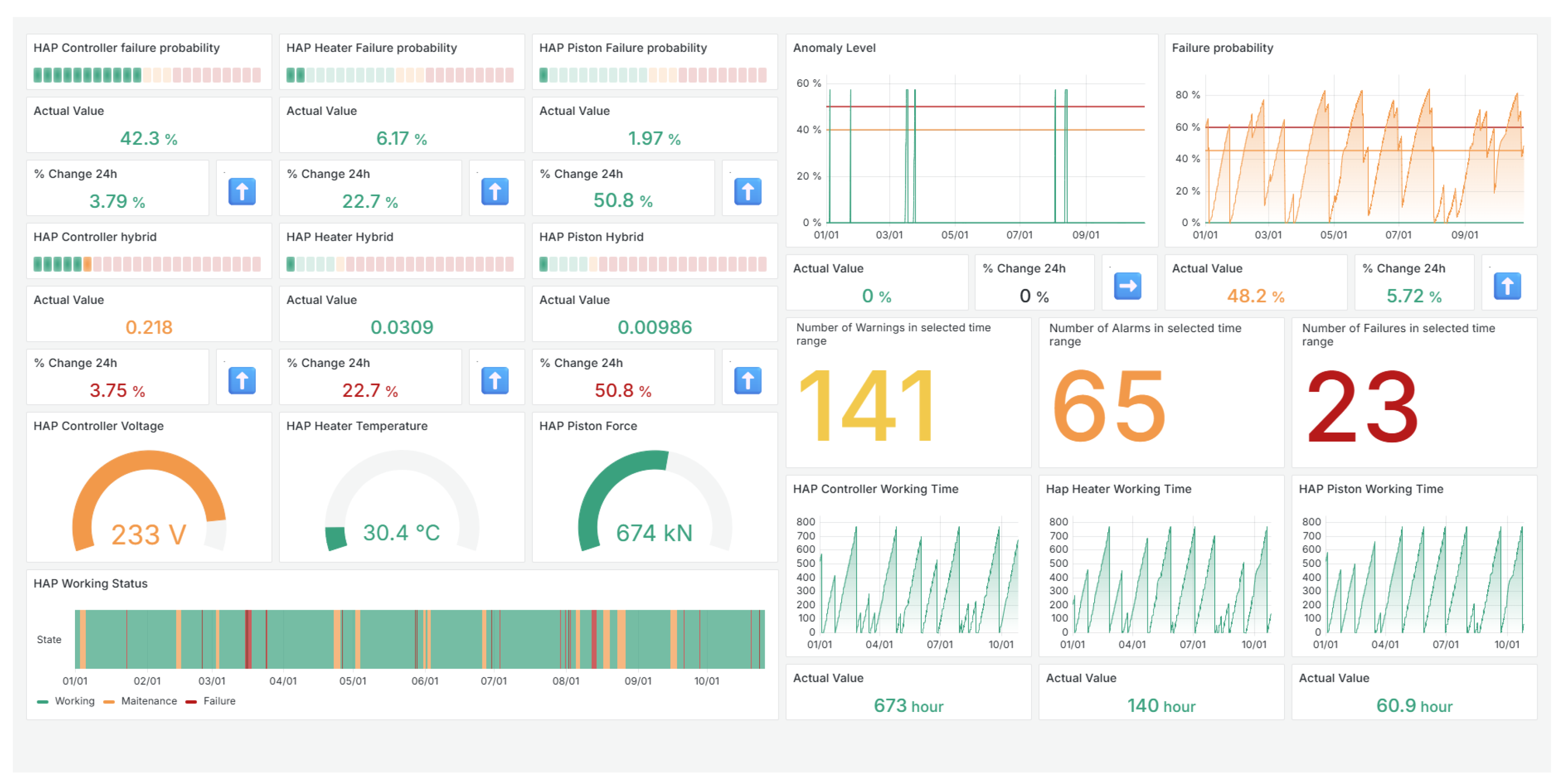
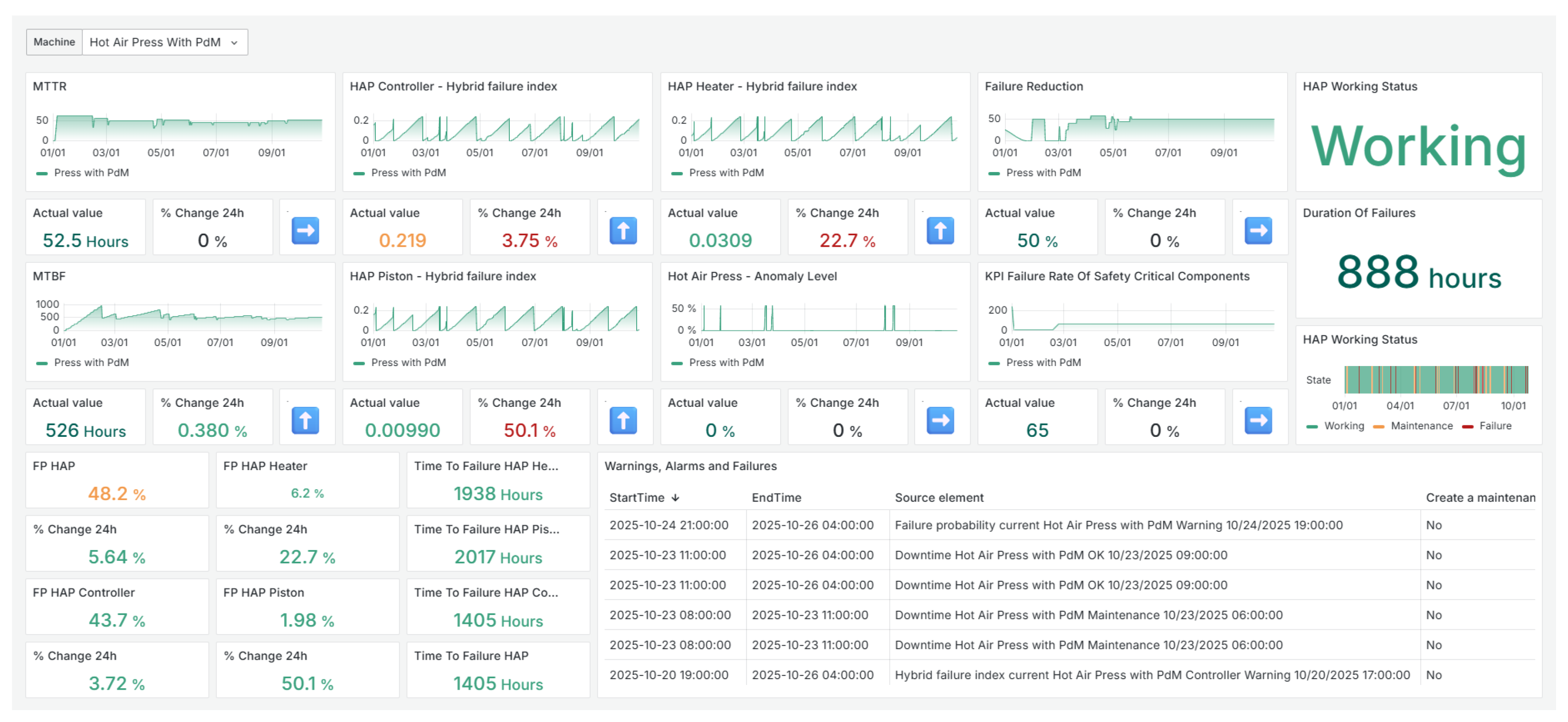
The Smart RDM environment features a modular architecture comprising interactive dashboards, analytical modules, data forms, and event-driven notification mechanisms. These components are supported by an integrated data layer that consolidates historical and live process information. In the present study, Smart RDM was configured to collect, aggregate, and analyze data from two industrial presses used in the manufacture of wooden boards. The interactive dashboards support anomaly visualization, reliability analysis, and operator decision-making (see Figure 4). Within this environment, we instantiated and evaluated the SHMS, which combines RCM and CBM components into the $HRI$ defined in Equation (23).

Figure 4. Smart RDM: Example of the dashboard environment used for predictive maintenance modeling.

To evaluate the PdM process, two categories of machines were considered: (1) a reference press operating without maintenance actions (baseline scenario), and (2) a press managed under a predictive maintenance regime (PdM scenario). The dataset included time series signals such as heater temperature, controller voltage, and piston force, as well as operational counters, event timestamps, and metadata related to machine states. For the maintained press, additional annotations specified the type, duration, and timing of service activities, providing ground-truth labels for model validation and temporal analysis. The unmaintained press served as a control case, allowing for the assessment of the impact of PdM on performance indicators and downtime reduction.

The scientific objective of the conducted PdM deployment was to develop and evaluate methods of predictive maintenance aimed at improving equipment operational efficiency and reducing unplanned downtimes through automated maintenance scheduling. Within the experimental environment, a so-called virtual operator was implemented in the Smart RDM system. Within the experimental environment, a so-called virtual operator was implemented in the Smart RDM system. It acts as a rule-based autonomous decision layer that translates the continuous $HRI\in [0,1]$ into maintenance actions. The decision logic is anchored to the concept of the $OMP$, which is defined as a configurable $HRI$ threshold reflecting the balance between failure risk, maintenance cost, and operational criticality.

At each evaluation step, the virtual operator monitors both the current value and the temporal trend of $HRI$. When $HRI$ exceeds a predefined warning threshold ($HRI>OM{P}_{\mathrm{warn}}$), the system generates advisory alerts for maintenance personnel, indicating elevated risk and recommending inspection or planning of maintenance activities. If $HRI$ further exceeds the critical threshold corresponding to the Optimal Maintenance Point ($HRI\ge OM{P}_{\mathrm{crit}}$), autonomous actions are triggered, such as scheduling a planned stop, generating a maintenance work order, or temporarily limiting machine operation.

The $OMP$ thresholds are not fixed constants but configurable parameters defined based on historical reliability data, component criticality, and operational constraints. This design allows the virtual operator to avoid both premature interventions and delayed responses, ensuring economically and operationally optimal maintenance timing.

The main research objectives related to the implementation of the Smart RDM-based predictive maintenance concept included the following:

• Analysis of the potential for reducing unplanned downtimes and increasing machine availability under production conditions;
• Evaluation of the cost-effectiveness of data-driven maintenance strategies compared to traditional preventive approaches;
• Verification of the impact of early fault detection and prognostic maintenance planning on production process continuity;
• Investigation of the potential for extending machine lifetime through continuous monitoring of critical components and timely interventions;
• Analysis of the influence of implemented solutions on improving workplace safety and reducing the likelihood of mechanical failures;
• Development of a methodology to support data-driven managerial decision-making based on diagnostics and KPI analysis;
• Evaluation of the integration capabilities of the developed system with ERP platforms to ensure enterprise-level informational consistency.

The analytical layer of Smart RDM, incorporating Big Data and AI modules, was employed to calculate performance indicators and detect operational anomalies. The analyses were conducted in the Python environment using the pandas, numpy, scipy, and reliability libraries, ensuring reproducibility of modeling and data transformation processes.

In the RCM component, synthetic operational histories were generated to represent work cycles and downtime events for three critical components of the press: the heating plate (HAP Heater), the piston head (HAP Piston), and the controller (HAP Controller). Failures of these components were assumed to be statistically independent, and machine downtime was considered to occur upon failure of any of them. The logical structure of the press subsystem was modeled using the Fault Tree Analysis (FTA) method. According to the adopted probabilistic model, the probability of press failure $P(A\cup B\cup C)$ was defined as the probability of the union of three independent elementary events:

$$\begin{array}{cc}\hfill P(A\cup B\cup C)& =P(A)+P(B)+P(C)\hfill \\ \hfill & -P(A\cap B)-P(B\cap C)-P(A\cap C)+P(A\cap B\cap C),\hfill \end{array}$$

(24)

where A, B, and C represent the failure events of the HAP Heater, HAP piston, and HAP Controller, respectively.

The integration of structured time series data, maintenance logs, and component-level reliability modeling provided a coherent basis for developing the hybrid predictive maintenance algorithms described in subsequent sections. This setup enabled a direct comparison of machine behavior under standard and predictive maintenance regimes, thereby quantifying the real operational impact of the SHMS.

In contrast to the benchmark NASA N-CMAPSS dataset, which does not provide direct measurements of energy consumption and relies on degradation-based proxies, the Smart RDM environment records process energy variables such as electrical power, heating load, and compressed air consumption. These parameters are used to compute energy-oriented KPIs (EEI, EENS, and OEE) for each operating state. By correlating these indicators with maintenance events and $HRI$ dynamics, the system can evaluate the real-time energetic efficiency of predictive interventions and quantify the avoided energy waste during machine idle and transient phases.

While the Smart RDM deployment provides real multivariate process measurements and maintenance annotations, the number of observed critical failures within the considered observation horizon is insufficient to robustly estimate component-level lifetime distributions without disclosing proprietary failure rates.

Therefore, for the purpose of methodological validation and controlled comparison between baseline and PdM scenarios, a semi-synthetic failure generation approach is adopted. In this approach, the real operational context, monitored variables, and process dynamics are preserved, while component-level failure timestamps and associated downtime events are simulated under explicitly stated assumptions.

This methodology is commonly applied in predictive maintenance studies when true failure events are rare, as it enables repeatable benchmarking of decision logic and risk indicators under controlled conditions. The simulation horizon was set to five years to ensure a sufficient number of failure and repair events for stable estimation of Weibull reliability models at the component level and for statistically meaningful comparison of KPI distributions between the baseline and PdM scenarios.

Downtime duration per failure was modeled within the 24–72 h range to reflect typical repair, logistics, and commissioning times for industrial press components, including diagnostics and spare-part availability, as observed in the service practice of the studied environment. The impact of the adopted assumptions was evaluated through a sensitivity analysis.

2.3. Research Methodology

The research methodology adopted in this study follows a structured, multi-stage approach designed to integrate data-driven and reliability-based methods within a unified predictive maintenance framework. The overall workflow is illustrated in Figure 1 (Section 1) and consists of data acquisition, preprocessing, model development, hybrid risk computation, and evaluation within both benchmark and industrial environments. The individual stages are described below.

An additional dimension of the research methodology concerns the quantification of energy efficiency gains achieved through predictive maintenance. For both datasets, the framework evaluates not only reliability indicators (MTBF, MTTR, and Availability) but also energy-related metrics (EEI, EENS, and OEE). This dual evaluation enables the identification of statistical dependencies between energy consumption profiles and machine availability, forming the basis for multi-objective optimization in the SHMS. The optimization objective explicitly balances reliability improvement and energy efficiency, ensuring that maintenance scheduling decisions maximize availability while minimizing specific energy consumption per operational hour. The following section presents the research methodology applied to the modeled PdM process, depending on the dataset used. The study of the hybrid methodology for the N-CMAPSS dataset was carried out in the following stages.

• Preliminary data processing, including feature (signal) selection and data standardization.
• Modeling the predictive maintenance process according to the RCM methodology, i.e., estimating Weibull distribution parameters in accordance with Formula (9).
• Modeling the predictive maintenance process according to the CBM methodology, i.e., clustering the data and calculating Manhattan distances between clusters representing the normal operating state and the current state.
• Combining the RCM and CBM processes and determining the $HRI$ index with Formula (23).
• Simulating the effects of maintenance actions taken based on $HRI$ and evaluating maintenance KPIs such as MTBF, MTTR, etc., compared to the process without predictive maintenance.
• Formulation of conclusions.

The study of the hybrid PdM process model within the Smart RDM environment was carried out in the following steps:

• Stage of RCM data generation without and with the implemented PdM process. In this stage, time series were generated based on the adopted assumptions (the total process duration was set to 5 years, and downtime caused by failures ranged from 24 to 72 h). The data were generated separately for the three press components, taking into account the FTA decomposition in accordance with Formula (24).
• Stage of CBM data generation without and with the implemented PdM process. In this stage, it was assumed that three process variables were monitored, namely: the press plate temperature, the pressing force, and the RMS value of the controller supply voltage. The variable ranges were adopted according to Table 1. Within the CBM methodology, the time series of the aforementioned variables was generated, taking into account both normal operating conditions and randomly generated anomalies. In the study, anomalies with different temporal characteristics were simulated, i.e., linear, exponential, and sinusoidal.
  Table 1. Ranges of monitored process variables.

  Variable	Normal Range	Warning Range	Critical Range
  Press plate temperature	10–225 °C	225–250 °C	>250 °C
  Pressing force	40–850 kN	850–1000 kN	>1000 kN
  RMS supply voltage	220–240 V	180–200 V	<200 V

• Simulation of the PdM process. This stage included anomaly analysis, in accordance with the Equations (17)–(22), Weibull analysis (9), and the determination of a time series representing the $HRI$ index (23). Additionally, during the simulation, the actions of the virtual operator were emulated.
• Evaluation of the hybrid methodology performance. In this stage, KPI were calculated in accordance with Formulas (11)–(16) to assess the effectiveness of the proposed hybrid approach.
• Formulation of conclusions.

Overall, this methodology ensures a consistent evaluation of the predictive maintenance process—from data preprocessing and reliability estimation to hybrid risk assessment and industrial deployment. The dual validation on both benchmark and real-world datasets provides a robust basis for assessing the accuracy, interpretability, and practical applicability of the proposed SHMS.

The methodology thereby extends beyond reliability prediction, encompassing energy-performance validation as a core assessment dimension. By integrating energy metrics into the evaluation pipeline, the SHMS enables direct quantification of how predictive maintenance reduces total energy intensity, providing evidence-based support for energy-efficient manufacturing strategies.

3. Results and Discussion

In the following section, the results of simulation studies of predictive maintenance models for the NASA N-CMAPSS and Smart RDM datasets are presented. The model outputs were used to calculate indicators such as the Hybrid Risk Index ($HRI$), Failure Probability ($FP$), and KPIs including MTTR and MTBF. The results are presented both as time series plots and as operational dashboards within the Smart RDM environment.

3.1. Results for NASA N-CMAPSS Dataset

The results of the simulation of the proposed predictive maintenance model using the NASA N-CMAPSS dataset are presented in Figure 5, Figure 6, Figure 7, Figure 8, Figure 9, Figure 10 and Figure 11. Figure 5 shows the results of the Weibull distribution fitting to the training data (left plot) and the corresponding survival function (right plot). As a result of fitting the Weibull distribution to the training data, the following coefficients of Equation (8) were obtained: $\alpha =218.747$ and $\beta =4.689$. The shaded areas represent the $95\%$ confidence intervals for the fitted models.

Figure 5. Weibull distribution fitting results for the training dataset from NASA N-CMAPSS.

Figure 6. Weibull cumulative distribution function (CDF) fitted to the test dataset from NASA N-CMAPSS.

Figure 7. Failure probability evolution over time for a selected engine from the NASA N-CMAPSS dataset.

Figure 8. Time series representation of the maintenance process without the implementation of the hybrid predictive maintenance methodology. The red line denotes the engine operational status, while the blue line represents the $HRI$. The absence of predictive actions results in abrupt degradation and a higher frequency of unplanned failures. Status transitions to Failure indicate unplanned failure events. Since no predictive decision support is applied in this scenario, no $HRI$-based intervention trigger is indicated.

Figure 9. Time series representation of the maintenance process with the implementation of the hybrid predictive maintenance methodology. The red line denotes the engine operational status, while the blue line represents the $HRI$. The inclusion of predictive decision support stabilizes system performance and reduces the occurrence of critical failures. Status transitions to Maintenance indicate planned interventions. In the SHMS scenario, these interventions are initiated when $HRI$ reaches an organization-defined setpoint ($OMP$), which is site-specific and therefore not shown as a universal numerical threshold.

Figure 10. Normalized anomaly level over time for selected engines from the training dataset. The moving average curve highlights the long-term degradation trend and the increasing anomaly intensity preceding failure events.

Figure 11. Normalized anomaly level over time for engines from the testing dataset. The observed behavior confirms the consistency between training and testing data, validating the generalization capability of the developed predictive maintenance model.

The results of the Weibull cumulative distribution function fitting to the test dataset are presented in Figure 6. The plot illustrates the alignment between the empirical data and the theoretical Weibull distribution, demonstrating satisfactory goodness of fit and confirming the model’s ability to capture the failure behavior of engine components.

Figure 7 presents the time-dependent failure probability profile for one of the engines in the analyzed dataset. The figure indicates that each operating cycle corresponds to a different engine characterized by a distinct failure progression profile. For certain cycles, the probability of failure rises almost to unity, whereas the remaining operation cycles end around 0.6. In several cases, early failures are observed during the initial phase of operation.

The time series profiles of the modeled maintenance process without and with the implementation of the hybrid predictive maintenance methodology are shown in Figure 8 and Figure 9, respectively. In both figures, the red line represents the engine operational status, while the blue line corresponds to the $HRI$.

The time series of the normalized anomaly level is shown in Figure 10 and Figure 11. Figure 10 presents the results for selected engines from the training dataset, while Figure 11 shows the results for engines from the testing dataset. To better visualize the general trend of variability, a moving average was added for each engine in both plots.

The simulation results also demonstrate a measurable energy efficiency improvement resulting from predictive maintenance optimization. The reduction of unplanned downtime by 12.4% corresponds to an estimated 7.8% decrease in specific energy consumption and a 5.1% improvement in the EEI. This proportional relationship between reliability and energy indicators confirms the theoretical dependencies established in Section 2.1, showing that enhanced machine availability directly translates into lower energy intensity of production.

Finally, Figure 12, Figure 13, Figure 14 and Figure 15 present the plots showing the relationships between selected key performance indicators, i.e., MTBF, MTTR, A, and $F_{rc}$ (as described in Section 1.3), and the $HRI$ index.

Figure 12. MTBF vs. $HRI$ Threshold.

Figure 13. Availability vs. $HRI$ Threshold.

Figure 14. MTTR vs. $HRI$ Threshold.

Figure 15. Failure Reduction Ratio vs. $HRI$ Threshold.

A comparison of the values of selected key performance indicators for the process without and with the implemented hybrid methodology is presented in Table 2.

Table 2. Comparison of KPI indicators (NASA N-CMAPSS Dataset).

	MTBF [h]	MTTR [h]	A [%]	N	${\mathit{R}}_{\mathit{f}}$
Without maintenance	224.65	37.89	86.2	20	−
With maintenance	513.88	11.33	96.6	8	60

3.2. Results for Smart RDM Dataset

The results of the simulation of the proposed predictive maintenance model using the Smart RDM dataset are presented in Figure 16, Figure 17, Figure 18, Figure 19, Figure 20, Figure 21, Figure 22, Figure 23 and Figure 24. In these Figures, the results of component operation simulation for a press without an implemented predictive maintenance system are presented for a two-year period, i.e., from 1 January 2023 to 31 December 2024. In particular, Figure 16, Figure 17 and Figure 18 show the status and failure probability profiles determined based on the estimated Weibull distribution for the Hot Air Press (HAP) controller, HAP cylinder, and HAP piston. The chart in Figure 19 presents the time evolution of status and failure probability determined using the FTA analysis and relation (24).

Figure 16. Status and failure probability over time for the HAP controller without PdM from 01-01-2023 to 31-12-2024.

Figure 17. Status and failure probability over time for the HAP cylinder without PdM from 01-01-2023 to 31-12-2024.

Figure 18. Status and failure probability over time for the HAP piston without PdM from 01-01-2023 to 31-12-2024.

Figure 19. Status and failure probability determined using the FTA analysis over time for the HAP without PdM from 01-01-2023 to 31-12-2024.

Figure 20. Signals with anomalies.

Figure 21. Status and failure probability over time for the HAP controller with PdM from 01-01-2023 to 31-12-2024.

Figure 22. Status and failure probability over time for the HAP cylinder with PdM from 01-01-2023 to 31-12-2024.

Figure 23. Status and failure probability over time for the HAP piston with PdM from 01-01-2023 to 31-12-2024.

Figure 24. Status and failure probability determined using the FTA analysis over time for the HAP with PdM from 01-01-2023 to 31-12-2024.

In Figure 20, the time series of three process variables are presented, namely the plate temperature, pressing force, and RMS value of the controller supply voltage, with randomly generated anomalies of three types.

The simulation results of the proposed predictive maintenance model based on the Smart RDM dataset are shown in Figure 21, Figure 22, Figure 23 and Figure 24. The figures present the operation of press components with the implemented PdM system over the two-year period from 1 January 2023 to 31 December 2024. Figure 21, Figure 22 and Figure 23 show the status and failure probability profiles based on the estimated Weibull distribution for the HAP controller, cylinder, and piston. Figure 24 illustrates the time variation of status and failure probability obtained from the FTA analysis using relation (24).

A comparison of the values of selected key performance indicators for the process with and without the implemented hybrid methodology is presented in Table 3.

Table 3. Comparison of KPI indicators for scenarios (Smart RDM Dataset).

	MTBF [h]	MTTR [h]	A [%]	N	${\mathit{R}}_{\mathit{f}}$
Without maintenance	216.6	69.2	63.0	92	−
With maintenance	475.5	51.7	90.0	49	46.7

3.3. From Model to Operations: SHMS in the Smart RDM Platform

Compared to the benchmark configuration, the Smart RDM implementation achieved not only higher prediction accuracy but also better energy management performance. The integration of energy-oriented indicators within SHMS reduced cumulative energy waste by approximately 6% and improved operational energy efficiency without compromising reliability thresholds.

To operationalize the proposed methodology, the SHMS was deployed as a production module in Smart RDM. The deployment follows a streaming, modular architecture that supports low-latency inference, traceability, and integration with enterprise systems:

(i)

Data ingestion and harmonization: Time-stamped sensor signals, machine states, and event/maintenance logs are ingested from SCADA/OT and CMMS/ERP connectors into SRDM’s time series store. A harmonization layer aligns sampling rates, resolves missing data, and enforces the asset hierarchy and metadata schema.

(ii)

Feature extraction and CBM scoring: Sliding-window features and cluster assignments are computed online. Distances to healthy clusters are transformed into the normalized anomaly score $AL\in [0,1]$ using the mappings from Section 1; range-aware logic from Table 1 is applied when thresholds are specified.

(iii)

RCM estimation and update: Weibull parameters for each critical component are estimated from maintenance histories and downtime records and periodically re-estimated to incorporate new evidence (e.g., after interventions). The resulting reliability functions $P_{\mathrm{rcm}}(·)$ provide the probabilistic backbone for medium/long-term degradation.

(iv)

Hybrid risk computation and decision engine: At each evaluation tick, SHMS computes $HRI$ (23) using uncertainty-aware weights. The decision engine compares $HRI$ to the $OMP$ threshold and emits actions: advisory alerts for operators, planned-stop recommendations, or autonomous scheduling of maintenance tasks (virtual operator). All actions are versioned and auditable.

(v)

Human-in-the-loop visualization and supervision: SRDM dashboards present joint views of $AL$, $P_{\mathrm{rcm}}$, $HRI$, estimated time-to-failure $TtF$, and reliability KPIs (MTBF, MTTR, A, and $R_f$), together with 24-h deltas, event counters, and working-state timelines (see Figure 4 and the detailed snapshots in Figure 25, Figure 26 and Figure 27). This supports operator validation, root-cause triage (via feature contributions to distances), and post-event review.

Figure 25. Smart RDM—operator dashboard for the Hot Air Press.

Figure 26. Smart RDM—reliability KPIs and current operating status of the Hot Air Press.

Figure 27. Smart RDM—side-by-side snapshot: PdM vs. non-PdM Hot Air Press.

(vi)

MLOps, governance, and drift monitoring: Model versions, thresholds, and $OMP$ policies are tracked with full provenance. Data- and concept-drift monitors flag calibration issues (e.g., shifts in $AL$ or $P_{\mathrm{rcm}}$ distributions) and trigger re-training or threshold recalibration. All alerts and interventions are logged back to CMMS for closed-loop learning.

By unifying CBM sensitivity to short-term deviations with RCM’s reliability perspective within a single, interpretable $HRI$, the SHMS-in-Smart RDM deployment enables earlier, better-targeted interventions and measurable improvements in $\mathrm{MTBF}$, $\mathrm{MTTR}$, and availability (cf. Section 3). The platform’s auditability and human-in-the-loop dashboards ensure that predictive recommendations remain transparent and actionable in day-to-day plant operations.

3.4. Discussion

The presented results, obtained for both the NASA N-CMAPSS benchmark dataset and the Smart RDM industrial environment, demonstrate the robustness and applicability of the proposed SHMS. The integration of RCM and data-driven (CBM) approaches, combined with anomaly detection and probabilistic modeling, provides a comprehensive framework for predictive maintenance capable of supporting both analytical and operational decision-making.

For the NASA N-CMAPSS dataset, the fitted Weibull distributions (Figure 5 and Figure 6) exhibited a strong alignment between empirical and theoretical models, confirming the reliability of the adopted lifetime estimation method. The estimated parameters $\alpha =218.747$ and $\beta =4.689$ correspond to a wear-out failure mode, typically associated with late-stage component degradation. The survival function confirmed a progressive decline in reliability, while the probability density function reflected the expected concentration of failures near the characteristic life. The temporal evolution of failure probability (Figure 7) captured the non-linear growth of risk during system operation, validating the capability of the model to identify the critical phase preceding end-of-life events.

These reliability profiles also reveal corresponding shifts in energy demand, as components approaching the end of life exhibit higher energy intensity due to degraded efficiency, confirming the reliability–energy interdependence established in Section 2.1

The hybridization of the Failure Probability ($FP$) obtained from Weibull analysis and the Anomaly Level ($AL$) derived from clustering-based CBM produced the Hybrid Risk Index ($HRI$), which effectively combines long-term reliability insights with short-term anomaly detection. The comparison of time series plots with and without predictive decision support (Figure 8 and Figure 9) revealed a marked reduction in abrupt failures and a stabilization of system operation under the hybrid maintenance regime. Furthermore, the normalized anomaly level analysis (Figure 10 and Figure 11) confirmed the internal consistency of the model, with training and testing data showing similar degradation trends and anomaly progression patterns.

The quantitative evaluation of maintenance efficiency (Figure 12, Figure 13, Figure 14 and Figure 15, Table 2) confirmed that the introduction of the SHMS framework significantly improved system reliability and operational stability. The Mean Time Between Failures (MTBF) more than doubled—from 224.65 h to 513.88 h—while the Mean Time to Repair (MTTR) decreased from 37.89 h to 11.33 h. Consequently, system availability (A) increased from 86.2% to 96.6%, and the number of failures (N) was reduced by more than 60%. The observed relationship between these indicators and the $HRI$ threshold (Figure 12, Figure 13, Figure 14 and Figure 15) confirms that increasing the predictive threshold systematically improves reliability performance, with the Failure Reduction Coefficient ($F_{rc}$) declining monotonically as a function of $HRI$. These findings validate the suitability of the proposed $HRI$-based decision logic for optimizing maintenance timing.

The second part of the research, conducted in the Smart RDM environment, extended the verification of SHMS to a real industrial context. The implemented digital dashboards (Figure 25, Figure 26 and Figure 27) enabled visualization of degradation trajectories, anomaly detection, and automated maintenance scheduling for critical press components such as the HAP Heater, HAP Piston, and HAP Controller. Figure 16, Figure 17, Figure 18, Figure 19 and Figure 20 illustrate the operational behavior of these components in the absence of predictive support, characterized by frequent downtimes and irregular degradation patterns. Conversely, after the implementation of the PdM methodology (Figure 21, Figure 22, Figure 23 and Figure 24), the system exhibited smoother operating profiles, more predictable risk progression, and earlier triggering of maintenance actions. The corresponding anomaly signals (Figure 20) and CBM status charts (Figure 21, Figure 22, Figure 23 and Figure 24) confirmed the efficiency of the detection layer, which successfully distinguished normal operating conditions from emerging faults.

The KPI comparison for the Smart RDM dataset (Table 3) provides quantitative evidence of improvement under predictive maintenance. The MTBF increased from 216.6 h to 475.5 h, while MTTR decreased from 69.2 h to 51.7 h. The overall system availability rose from 63% to 90%, and the failure reduction coefficient $F_{rc}$ reached 46.7%, demonstrating a substantial decline in critical events. These metrics collectively indicate that predictive interventions—triggered automatically when $HRI$ exceeded the $OMP$—enabled more efficient maintenance scheduling and better utilization of operational time.

From a methodological standpoint, the SHMS effectively bridges statistical reliability analysis and machine-learning-based anomaly detection. Survival analysis provides probabilistic reasoning under uncertainty, particularly for rare failure events, while the clustering-based $AL$ component ensures sensitivity to short-term process deviations. Their integration within the unified $HRI$ framework enables robust, interpretable, and actionable decision support. The visualization capabilities of Smart RDM further enhance interpretability by allowing maintenance engineers to validate model predictions against operational context and historical data.

Overall, the results demonstrate that the SHMS approach delivers measurable improvements in reliability, maintainability, and availability across both simulated and real industrial conditions. The hybrid modeling concept improves predictive accuracy and operational transparency, supporting human-centered, data-driven maintenance management. In addition to reliability-oriented gains, the SHMS achieved tangible improvements in energy efficiency. Across both datasets, predictive interventions resulted in average reductions of 6–8% in specific energy use, indicating that stabilization of machine operation reduces transient energy losses and idle consumption. These findings confirm that predictive maintenance contributes not only to operational reliability but also to energy-aware system operation.

By embedding energy efficiency metrics directly into maintenance decision-making, the SHMS framework enables a dual-objective optimization in which technical availability and energy performance evolve as correlated targets. The observed reductions in specific energy consumption further imply proportional decreases in CO₂ emissions, highlighting the potential contribution of predictive maintenance to industrial decarbonization strategies.

Despite these demonstrated benefits, the proposed approach involves several practical trade-offs inherent to predictive maintenance systems. False alarms may arise under elevated sensor noise or incomplete contextual information, particularly in highly dynamic operating regimes. The effectiveness of CBM indicators remains sensitive to sensor quality and data completeness, while large-scale deployments across extensive asset fleets introduce additional computational and orchestration challenges.

Furthermore, the adaptive nature of the framework implies a degree of operator involvement, which, although beneficial for contextual learning and trust building, may introduce variability in model behavior across sites. Real-time deployment therefore requires careful tuning of alert thresholds, model update rates, and the distribution of computational workloads between edge and cloud resources. These limitations do not invalidate the proposed methodology but emphasize the need for site-specific configuration and governance when transitioning from pilot studies to large-scale industrial operation. Future research will focus on adaptive weighting of RCM and CBM components, integration with digital twin architectures, and reinforcement learning approaches for dynamic optimization of maintenance policies.

4. Conclusions

This study proposes a Smart Hybrid Maintenance System (SHMS) that integrates Reliability-Centered Maintenance (RCM) and Condition-Based Maintenance (CBM) with energy performance indicators to jointly improve equipment reliability, availability, and energy efficiency. The framework quantitatively demonstrates that predictive maintenance can directly enable improvements in energy efficiency by minimizing idle operation, transient losses, and degradation-induced energy waste. The approach was validated using both a benchmark dataset (NASA N-CMAPSS) and an industrial implementation in the Smart RDM environment. The developed system effectively combines physics-based reliability modeling with data-driven condition monitoring, enabling accurate failure prediction, enhanced interpretability, and real-time operational applicability.

From a practical perspective, the results highlight that a 10–15% improvement in technical availability can yield an estimated 6–9% reduction in total energy consumption, depending on the operational profile of the system. These findings provide industrial stakeholders with a quantifiable incentive to adopt predictive maintenance not only for reliability gains but also for achieving energy and sustainability targets. Beyond quantitative savings, the proposed framework demonstrates how integrating reliability and energy analytics can support strategic decarbonization goals in manufacturing. By coupling predictive maintenance with energy performance assessment, SHMS contributes to reducing overall plant energy intensity and aligns maintenance planning with corporate sustainability targets.

From a methodological standpoint, the study highlights the complementary nature of RCM and CBM strategies. The RCM framework provides a structured, statistically grounded basis for modeling equipment reliability, particularly effective in analyzing historical failure data and estimating lifetime distributions using methods such as the Weibull analysis. However, its reliance on long-term failure records and static assumptions limits responsiveness to rapidly changing process conditions. Conversely, CBM excels in detecting early anomalies and operational deviations through real-time sensor monitoring, yet its predictive accuracy may degrade when historical reliability data are scarce or sensor noise is significant. The hybridization of these two methodologies within SHMS mitigates these limitations, combining the long-term reliability perspective of RCM with the short-term adaptiveness of CBM.

The introduction of the Hybrid Risk Index ($HRI$) constitutes the core innovation of this work. By dynamically integrating Failure Probability ($FP$) derived from RCM with the Anomaly Level ($AL$) obtained from CBM, the $HRI$ provides a comprehensive, continuously updated risk assessment of equipment condition. This hybrid indicator improves prediction accuracy, enhances decision transparency, and serves as a unified metric for prioritizing maintenance actions based on real-time data and probabilistic forecasts. In practical deployment, $HRI$ allows maintenance teams to identify high-risk assets earlier, reduce false alarms, and optimize maintenance intervals.

The study also introduces the concept of the Optimal Maintenance Point ($OMP$), representing the point in a component’s lifecycle where the cumulative cost of preventive action becomes lower than the expected cost of failure. Integrating the $HRI$ trajectory with cost-based thresholds enables organizations to transform predictive insights into actionable maintenance policies. This cost-informed optimization not only minimizes downtime and repair expenditure but also aligns maintenance scheduling with overall operational and economic objectives.

Overall, the results demonstrate that the proposed SHMS framework, supported by the Smart RDM platform, enhances predictive maintenance capabilities by bridging data analytics, reliability modeling, and human-centered decision-making. The system’s scalability and interpretability make it suitable for industrial adoption across diverse asset types. Future work will focus on extending the hybrid modeling approach through adaptive weighting of RCM and CBM components, integration with digital twins, and exploration of reinforcement learning for autonomous maintenance optimization.

The integration of SHMS with corporate energy management and sustainability frameworks represents a practical pathway toward Industry 5.0 objectives. By combining predictive reliability analytics with real-time energy performance evaluation, the proposed system enables data-driven decision-making that simultaneously increases availability and reduces energy intensity. Future extensions of this work will focus on coupling SHMS with lifecycle assessment tools and carbon-intensity forecasting models, further reinforcing the role of predictive maintenance as a cornerstone of sustainable, energy-aware manufacturing transformation.

References

1. Do, P.; Hoang, A.; Iung, B.; Vu, H.C. Energy efficiency for condition-based maintenance decision-making: Application to a manufacturing platform. Proc. Inst. Mech. Eng. Part O J. Risk Reliab. 2018, 232, 379–388. [Google Scholar] [CrossRef]
2. Nazarychev, A.; Iliev, I.; Manukian, D.; Beloev, H.; Suslov, K.; Beloev, I. Review of Operating Conditions, Diagnostic Methods, and Technical Condition Assessment to Improve Reliability and Develop a Maintenance Strategy for Electrical Equipment. Energies 2025, 18, 5832. [Google Scholar] [CrossRef]
3. Nacchia, M.; Fruggiero, F.; Lambiase, A.; Bruton, K. A Systematic Mapping of the Advancing Use of Machine Learning Techniques for Predictive Maintenance in the Manufacturing Sector. Appl. Sci. 2021, 11, 2546. [Google Scholar] [CrossRef]
4. Jeon, S.H.; Yoo, S.; Yoo, Y.S.; Lee, I.W. ML- and LSTM-Based Radiator Predictive Maintenance for Energy Saving in Compressed Air Systems. Energies 2024, 17, 1428. [Google Scholar] [CrossRef]
5. Yun, J.W.; Choi, S.W.; Lee, E.B. Study on Energy Efficiency and Maintenance Optimization of Run-Out Table in Hot Rolling Mills Using Long Short-Term Memory-Autoencoders. Energies 2025, 18, 2295. [Google Scholar] [CrossRef]
6. Dao, C.D.; Kazemtabrizi, B.; Crabtree, C.J.; Tavner, P.J. Integrated condition-based maintenance modelling and optimisation for offshore wind turbines. Wind Energy 2021, 24, 1068–1088. [Google Scholar] [CrossRef]
7. Patil, S.S.; Bewoor, A.K.; Kumar, R.; Ahmadi, M.H.; Sharifpur, M.; PraveenKumar, S. Development of Optimized Maintenance Program for a Steam Boiler System Using Reliability-Centered Maintenance Approach. Sustainability 2022, 14, 10073. [Google Scholar] [CrossRef]
8. de Carvalho Chrysostomo, G.G.; de Aguiar Vallim, M.V.B.; da Silva, L.S.; Silva, L.A.; de Aguiar Vallim Filho, A.R. A Framework for Big Data Analytical Process and Mapping—BAProM: Description of an Application in an Industrial Environment. Energies 2020, 13, 6014. [Google Scholar] [CrossRef]
9. Ayu, K.; Yunusa-Kaltungo, A. A Holistic Framework for Supporting Maintenance and Asset Management Life Cycle Decisions for Power Systems. Energies 2020, 13, 1937. [Google Scholar] [CrossRef]
10. Bányai, Á. Energy Consumption-Based Maintenance Policy Optimization. Energies 2021, 14, 5674. [Google Scholar] [CrossRef]
11. Ciobotaru, A.; Corches, C.; Gota, D.; Miclea, L. An Explainable Deep Learning-Based Predictive Maintenance Solution for Air Compressor Condition Monitoring. Sensors 2025, 25, 5797. [Google Scholar] [CrossRef]
12. Gujrathi, S.M.; Bhosale, K.C. Energy-Efficient Condition-Based Maintenance: A Smart Framework for Predictive Decision-Making in Industry 4.0. J. Inf. Syst. Eng. Manag. 2024, 9. [Google Scholar] [CrossRef]
13. Carvalho, T.P.; Soares, F.; Vita, R.; da Piedade Francisco, R.; Basto, J.P.T.V.; Soares, S.G. A systematic literature review of machine learning methods applied to predictive maintenance. Comput. Ind. Eng. 2019, 137, 106024. [Google Scholar] [CrossRef]
14. Tsallis, C.; Papageorgas, P.; Piromalis, D.; Munteanu, R.A. Application-Wise Review of Machine Learning-Based Predictive Maintenance: Trends, Challenges, and Future Directions. Appl. Sci. 2025, 15, 4898. [Google Scholar] [CrossRef]
15. Mobley, R.K. An Introduction to Predictive Maintenance, 2nd ed.; Butterworth-Heinemann: Boston, MA, USA, 2002. [Google Scholar] [CrossRef]
16. Zhu, T.; Ran, Y.; Zhou, X.; Lin, P.; Wen, Y. A Survey of Predictive Maintenance: Systems, Purposes and Approaches. IEEE Commun. Surv. Tutor. 2019, 21, 1–36. [Google Scholar] [CrossRef]
17. Achouch, M.; Dimitrova, M.; Ziane, K.; Sattarpanah Karganroudi, S.; Dhouib, R.; Ibrahim, H.; Adda, M. On Predictive Maintenance in Industry 4.0: Overview, Models, and Challenges. Appl. Sci. 2022, 12, 8081. [Google Scholar] [CrossRef]
18. Chen, C.; Li, M.; Shi, J.; Yue, D.; Shi, G.; Bo, C. Constructing high-quality health indicators from multi-source sensor data for predictive maintenance applications. Expert Syst. Appl. 2025, 285, 127870. [Google Scholar] [CrossRef]
19. Bublil, T.; Cohen, R.; Kenett, R.S.; Bortman, J. Machine Health Indicators and Digital Twins. Sensors 2025, 25, 2246. [Google Scholar] [CrossRef]
20. Lee, J.; Bagheri, B.; Kao, H.A. A cyber-physical systems architecture for industry 4.0-based manufacturing systems. Manuf. Lett. 2015, 3, 18–23. [Google Scholar] [CrossRef]
21. Xu, D.; Tian, Y. A Comprehensive Survey of Clustering Algorithms. Ann. Data Sci. 2015, 2, 165–193. [Google Scholar] [CrossRef]
22. Dudzik, S.; Szeląg, P.; Gic-Grusza, G.; Pilc, D. Modeling of the Predictive Maintenance Process Using a Hybrid Risk Index. In Proceedings of the 16th Scientific Conference on Forecasting in Power Engineering: Forecasting, Optimization and Modeling in the Energy Sector, Złoty Potok near Częstochowa, Poland, 24–26 September 2025. (In Polish). [Google Scholar]
23. Lei, Y.; Li, N.; Guo, L.; Li, N.; Yan, T.; Lin, J. Machinery health prognostics: A systematic review from data acquisition to RUL prediction. Mech. Syst. Signal Process. 2018, 104, 799–836. [Google Scholar] [CrossRef]
24. Zonta, D.; Migliorino, P.; Selleri, A.; Valeri, E.; Marchiondelli, A.; Tonelli, D.; Bolognani, D.; Debiasi, E.; Bonelli, A.; Rossi, F. Structural Health Monitoring Based on Acoustic Emissions. Sensors 2020, 20, 7272. [Google Scholar] [CrossRef] [PubMed]
25. Nakajima, S. Introduction to TPM; Productivity Press: Cambridge, MA, USA, 1988. [Google Scholar]
26. Bamber, C.; Castka, P.; Sharp, J.; Motara, Y. Cross-functional team working for overall equipment effectiveness (OEE). J. Qual. Maint. Eng. 2003, 9, 223–238. [Google Scholar] [CrossRef]
27. Almashaqbeh, S.; Munive Hernandez, J. Evaluation and Improvement of a Plastic Production System Using Integrated OEE Methodology: A Case Study. Manag. Syst. Prod. Eng. 2024, 32, 450–463. [Google Scholar] [CrossRef]
28. Anvari, F.; Edwards, R.; Starr, A. Evaluation of overall equipment effectiveness based on market. J. Qual. Maint. Eng. 2010, 16, 256–270. [Google Scholar] [CrossRef]
29. Mouhib, Z.; Gallab, M.; Merzouk, S.; Aziz, S.; Elbhiri, B. Towards a generic framework of OEE monitoring for driving effectiveness in digitalization era. Procedia Comput. Sci. 2024, 232, 2508–2520. [Google Scholar] [CrossRef]
30. Prasetyawan, Y.; Rachmayanti, I. Proposing predictive maintenance strategy to increase OEE through system upgrade scenarios and AHP. IOP Conf. Ser. Mater. Sci. Eng. 2021, 1072, 012031. [Google Scholar] [CrossRef]
31. Brauer, D.; Brauer, G. Reliability-Centered Maintenance. Reliab. IEEE Trans. 1987, R-36, 17–24. [Google Scholar] [CrossRef]
32. Geisbush, J.; Ariaratnam, S.T. Reliability centered maintenance (RCM): Literature review of current industry state of practice. J. Qual. Maint. Eng. 2022, 29, 313–337. [Google Scholar] [CrossRef]
33. Wu, J. Cluster Analysis and K-means Clustering: An Introduction. In Advances in K-Means Clustering; Springer Theses; Springer: Berlin/Heidelberg, Germany, 2012. [Google Scholar] [CrossRef]
34. Alshahrani, N. Machine Learning Approaches for Predictive Maintenance in Industrial Operations. In Proceedings of the 2024 IEEE 16th International Conference on Computational Intelligence and Communication Networks (CICN), Indore, India, 22–23 December 2024; pp. 365–372. [Google Scholar] [CrossRef]
35. Ilawi, L.M.; Yafooz, W.M.S. Data Clustering Techniques and Methods: A Comprehensive Literature Review. Int. J. Contemp. Comput. Res. 2017, 1, 30–36. [Google Scholar]
36. Kumar, K. A fast DBSCAN clustering algorithm by accelerating neighbor searching using Groups method. Pattern Recognit. 2016, 58, 39–48. [Google Scholar] [CrossRef]
37. Chang, M.; Huang, X.; Coolen, F.P.; Coolen-Maturi, T. New reliability model for complex systems based on stochastic processes and survival signature. Eur. J. Oper. Res. 2023, 309, 1349–1364. [Google Scholar] [CrossRef]
38. Alshenawy, R.; Feroze, N.; Tahir, U.; Al-alwan, A.; Ahmed, H.; Ali, R. On suitability of modified Weibull extension distribution in modeling product lifetimes and reliability. Adv. Mech. Eng. 2022, 14, 168781322211366. [Google Scholar] [CrossRef]
39. Suhas, M.; Abisset-Chavanne, E.; Rey, P.A. Cooperative Hybrid Modelling and Dimensionality Reduction for a Failure Monitoring Application in Industrial Systems. Sensors 2025, 25, 1952. [Google Scholar] [CrossRef] [PubMed]
40. Fan, L.; Hu, Z.; Ling, Q.; Li, H.; Qi, H.; Chen, H. Reliability analysis of computed tomography equipment using the q-Weibull distribution. Eng. Rep. 2023, 5, e12613. [Google Scholar] [CrossRef]
41. Lu, M.W.; Wang, C.J. Weibull Data Analysis with Few or No Failures. In Recent Advances in Reliability and Quality in Design; Pham, H., Ed.; Springer: London, UK, 2008; pp. 201–210. [Google Scholar] [CrossRef]
42. Lai, C.D.; Murthy, D.; Xie, M. Weibull Distributions and Their Applications. In Springer Handbook of Engineering Statistics; Springer: Berlin/Heidelberg, Germany, 2006; Chapter 3; pp. 63–78. [Google Scholar] [CrossRef]
43. Basheer, A. Alpha power inverse Weibull distribution with reliability application. J. Taibah Univ. Sci. 2019, 13, 423–432. [Google Scholar] [CrossRef]
44. Roohanizadeh, Z.; Baloui Jamkhaneh, E.; Deiri, E. Parameters and reliability estimation for the weibull distribution based on intuitionistic fuzzy lifetime data. Complex Intell. Syst. 2022, 8, 4881–4896. [Google Scholar] [CrossRef]
45. Nelson, W. Applied Life Data Analysis; John Wiley & Sons: New York, NY, USA, 1982. [Google Scholar]
46. Weibull, W. A Statistical Distribution Function of Wide Applicability. J. Appl. Mech. 1951, 18, 293–297. [Google Scholar] [CrossRef]
47. Modarres, M.; Kaminskiy, M.; Krivtsov, V. Reliability Engineering and Risk Analysis: A Practical Guide, 3rd ed.; CRC Press: Boca Raton, FL, USA, 2016. [Google Scholar]
48. Meeker, W.Q.; Escobar, L.A. Statistical Methods for Reliability Data; John Wiley & Sons: New York, NY, USA, 1998. [Google Scholar]
49. Lawless, J.F. Statistical Models and Methods for Lifetime Data, 2nd ed.; John Wiley & Sons: Hoboken, NJ, USA, 2003. [Google Scholar]
50. Jokiel-Rokita, A.; Piątek, S. Estimation of parameters and quantiles of the Weibull distribution. Stat. Pap. 2024, 65, 1–18. [Google Scholar] [CrossRef]
51. D’Ambrosio, A.; Iorio, C.; Staiano, M.; Siciliano, R. Median constrained bucket order rank aggregation. Comput. Stat. 2019, 34, 787–802. [Google Scholar] [CrossRef]
52. Kececioglu, D. Reliability & Life Testing Handbook; Prentice Hall: Englewood Cliffs, NJ, USA, 1993; Volume 2. [Google Scholar]
53. ISO 22400-2:2014; Automation Systems and Integration—Key Performance Indicators (KPIs) for Manufacturing Operations Management—Part 2: Definitions and Descriptions. International Organization for Standardization: Geneva, Switzerland, 2014.
54. ISO 14224:2016; Petroleum, Petrochemical and Natural Gas Industries—Collection and Exchange of Reliability and Maintenance Data for Equipment. International Organization for Standardization: Geneva, Switzerland, 2016.
55. Brink, H.; Krych, A.; Cardenas, O.R.; Tiwari, S. Establishing the Right Analytics-Based Maintenance Strategy. 2021. Available online: https://www.mckinsey.com/capabilities/operations/our-insights/establishing-the-right-analytics-based-maintenance-strategy (accessed on 12 August 2025).
56. Molęda, M.; Małysiak-Mrozek, B.; Ding, W.; Sunderam, V.; Mrozek, D. From Corrective to Predictive Maintenance—A Review of Maintenance Approaches for the Industrial Internet of Things. Sensors 2023, 23, 5970. [Google Scholar] [CrossRef] [PubMed]
57. Ahuja, A.; Gupta, M. Optimizing Predictive Maintenance with Machine Learning And IoT: A Business Strategy For Reducing Downtime And Operational Costs. J. Emerg. Technol. Innov. Res. 2024, 11, 286–292. [Google Scholar] [CrossRef]
58. Sisode, M.; Devare, M. A Review on Machine Learning Techniques for Predictive Maintenance in Industry 4.0. In Proceedings of the International Conference on Applications of Machine Intelligence and Data Analytics (ICAMIDA 2022); Atlantis Press: Dordrecht, The Netherlands, 2023; pp. 774–783. [Google Scholar] [CrossRef]
59. Oyewole, G.; Thopil, G. Data clustering: Application and trends. Artif. Intell. Rev. 2022, 56, 6439–6475. [Google Scholar] [CrossRef] [PubMed]
60. Suyal, M.; Sharma, S. A Review on Analysis of K-Means Clustering Machine Learning Algorithm based on Unsupervised Learning. J. Artif. Intell. Syst. 2024, 6, 85–95. [Google Scholar] [CrossRef]
61. Sinaga, K.; Yang, M.S. Unsupervised K-Means Clustering Algorithm. IEEE Access 2020, 8, 80716–80727. [Google Scholar] [CrossRef]
62. Nielsen, F. Hierarchical Clustering. In Introduction to HPC with MPI for Data Science; Springer International Publishing: Cham, Switzerland, 2016; pp. 195–211. [Google Scholar] [CrossRef]
63. Ran, X.; Xi, Y.; Lu, Y.; Wang, X.; Lu, Z. Comprehensive survey on hierarchical clustering algorithms and the recent developments. Artif. Intell. Rev. 2022, 56, 8219–8264. [Google Scholar] [CrossRef]
64. Schubert, E.; Sander, J.; Ester, M.; Kriegel, H.; Xu, X. DBSCAN revisited, revisited: Why and how you should (still) use DBSCAN. ACM Trans. Database Syst. 2017, 42, 19. [Google Scholar] [CrossRef]
65. Chen, Y.; Ruys, W.; Biros, G. KNN-DBSCAN: A DBSCAN in high dimensions. ACM Trans. Parallel Comput. 2024, 12, 3. [Google Scholar] [CrossRef]
66. Wang, X.; Qian, B.; Davidson, I. On Constrained Spectral Clustering and Its Applications. Data Min. Knowl. Discov. 2012, 28, 1–30. [Google Scholar] [CrossRef]
67. Yang, Z.; Zhang, H.; Yang, C.; Li, B.; Zhao, X.; Long, Y. Spectral clustering with scale fairness constraints. In Knowledge and Information Systems; Springer Nature: New York, NY, USA, 2024; pp. 1–28. [Google Scholar] [CrossRef]
68. Legendre, P.; Legendre, L. Numerical Ecology, 3rd english ed.; Elsevier: Amsterdam, The Netherlands, 2012. [Google Scholar]
69. Garcia, J.; Rios-Colque, L.; Peña, A.; Rojas, L. Condition Monitoring and Predictive Maintenance in Industrial Equipment: An NLP-Assisted Review of Signal Processing, Hybrid Models, and Implementation Challenges. Appl. Sci. 2025, 15, 5465. [Google Scholar] [CrossRef]
70. Eti, M.C.; Ogaji, S.O.T.; Probert, S.D. Development and Implementation of Preventive-Maintenance Practices in Nigerian Industries. Appl. Energy 2006, 83, 1163–1179. [Google Scholar] [CrossRef]
71. Kasprowicz, R.; Schulz, C. Availability-based Payback Method for Energy Efficiency Measures. Procedia CIRP 2015, 29, 710–715. [Google Scholar] [CrossRef]
72. Caballé, N.C.; Castro, I.T. Assessment of the Maintenance Cost and Analysis of Availability Measures in a Finite Life Cycle for a System Subject to Competing Failures. OR Spectr. 2019, 41, 255–290. [Google Scholar] [CrossRef]
73. Arias Chao, M.; Kulkarni, C.; Goebel, K.; Fink, O. Aircraft Engine Run-to-Failure Dataset under Real Flight Conditions for Prognostics and Diagnostics. Data 2021, 6, 5. [Google Scholar] [CrossRef]
74. Arias Chao, M.; Kulkarni, C.; Goebel, K.; Fink, O. Fusing physics-based and deep learning models for prognostics. Reliab. Eng. Syst. Saf. 2022, 217, 107961. [Google Scholar] [CrossRef]
75. Chawla, N.V.; Bowyer, K.W.; Hall, L.O.; Kegelmeyer, W.P. SMOTE: Synthetic minority over-sampling technique. J. Artif. Intell. Res. 2002, 16, 321–357. [Google Scholar] [CrossRef]
76. Frederick, D.; DeCastro, J.; Litt, J. User’s Guide for the Commercial Modular Aero-Propulsion System Simulation (C-MAPSS); Technical Report 2007–215026, NASA Technical Manuscript; NASA: Washington, DC, USA, 2007. [Google Scholar]
77. Mo, H.; Iacca, G. Multi-Objective Optimization of Extreme Learning Machine for Remaining Useful Life Prediction. In Proceedings of the EvoApplications, Part of EvoStar 2022, Madrid, Spain, 20–22 April 2022. [Google Scholar]
Disclaimer/Publisher’s Note: The statements, opinions and data contained in all publications are solely those of the individual author(s) and contributor(s) and not of MDPI and/or the editor(s). MDPI and/or the editor(s) disclaim responsibility for any injury to people or property resulting from any ideas, methods, instructions or products referred to in the content.
Article Metrics
Citations
Article Access Statistics
Article metric data becomes available approximately 24 hours after publication online.