Application of the Directed Cone Method for the Identification of Mathematical Models of Electromechanical Systems

Abstract

Electromechanical systems are inherently hybrid in nature, combining electrical and mechanical processes, and their increasing complexity requires the development of universal and computationally efficient mathematical models. In this study, we propose a macromodeling approach that represents the electromechanical system as a “black box,” in which internal physical processes are disregarded and the system behavior is defined solely by the relationship between input and output signals. The identification of such macromodels is reduced to solving a nonlinear optimization problem. To address this challenge, the directed cone method is applied, which searches for the global minimum of the objective function through stochastic movement across the hyperplane defined by the optimization problem. Several algorithmic improvements of the directed cone method are investigated, including step-size adaptation, simultaneous adaptation of step size and hypercone opening angle, and a tunneling procedure. Their effectiveness is evaluated using the construction of a macromodel of a single-phase asynchronous motor as a case study. Performance was assessed according to computational complexity (measured as the number of objective function evaluations until convergence), relative modeling accuracy, and the dynamics of progression toward the global minimum. The experimental results show that the tunneling-based algorithm provides the highest modeling accuracy with the lowest computational cost, whereas the step-size-only adaptation was found to be the least effective. The proposed approach demonstrates the feasibility of constructing accurate macromodels of electromechanical systems that can be integrated into computer-aided modeling environments such as MATLAB/Simulink R2023b. Future work will focus on extending the approach to a broader class of electromechanical systems and developing hybrid algorithms to enhance robustness with respect to model nonlinearity.

1. Introduction

A significant proportion of modern devices used in everyday life can reasonably be considered hybrid systems, in which elements of different nature and operating principles are combined. A typical example of such systems is represented by electromechanical systems, which include both purely electrical or electronic units and units that generate corresponding mechanical actions. In general, the operation of these systems is based on the principles of electromechanical energy conversion [1].

Today, electromechanical systems are employed in a wide range of application domains. Their continuous increase in complexity is accompanied by structural and functional diversification, as well as integration with other technical subsystems [2,3]. This, in turn, stimulates the emergence of new research directions in the field of electromechanics, such as geo-electromechanics, helio-electromechanics, nano-electromechanics, structural electromechanics, and genetic electromechanics [1,4]. These directions significantly extend the scope of application of both existing and newly developed electromechanical systems and devices.

One of the research objects in this study is the single-phase induction motor, which possesses several advantages, including a simple and robust design, self-starting capability, low manufacturing and operating costs, wide applicability, and favorable operational characteristics such as minimal vibration and noise. These motors are widely used in various applications, including air ventilation systems, liquid pumping, conveyor line drives, packaging machinery, and household appliances such as refrigerators, mixers, and washing machines [5,6,7,8].

However, the global trend toward improving the energy efficiency of electrical equipment—particularly in household applications [9,10]—has intensified scientific interest in investigating the operating behavior of induction motors through mathematical modeling and simulation of their various modes of operation [11,12].

The analysis and synthesis of modern complex systems, including electromechanical systems and their integration with other subsystems, require the construction of appropriate mathematical models of individual elements, objects, or systems. It is evident that such models must be adequate in terms of the principles of system operation and the nature of the processes they describe. At the same time, the mathematical apparatus employed in these models should be compatible with contemporary computer-aided mathematical modeling environments, such as MATLAB/Simulink R2023b [13]. Furthermore, given the diversity of electromechanical systems, the development of universal approaches to their modeling remains highly relevant.

2. Review of Modeling Methods for Electromechanical Systems

The nature of any electromechanical system or object necessitates that their models account for both the electrical parameters of the elements and the dynamics of the mechanical parts, which are induced by the action of the magnetic field. Traditional modeling methods of electromechanical systems involve the simultaneous use of the mathematical apparatus typical of electrical circuit theory and mathematical relations describing magnetic field effects [14]. As a result, the overall mathematical model of the system, represented in the form of a set of strongly nonlinear differential equations, often becomes overly complex. Moreover, constructing such a model typically requires the introduction of simplifying assumptions that allow for a certain level of abstraction tailored to a selected operating mode of the system [15]. Consequently, this process demands a high level of expertise from the researcher, which limits the pool of potential users of such models. It is also important to note that electromechanical systems rarely operate autonomously; rather, they usually function as components of larger and more complex systems. Hence, the excessive complexity of their models can negatively impact the process of integrating them with models of other subsystems.

At present, many electromechanical systems and objects are modeled using computer-aided tools. For instance, the MATLAB/Simulink R2023b library contains models for various operating modes of a number of electromechanical objects. However, when constructing new models, the researcher must carefully analyze the detailed structure of the target system and specify the constraints associated with the selected operating mode. Furthermore, challenges related to the compatibility of models across different systems persist.

In our view, a macro-approach provides a more suitable framework for modeling electromechanical systems [16]. In this case, the entire system is treated as an indivisible “black box,” whose behavior is modeled on the basis of observations of input and output signals [17]. The resulting representation is commonly referred to as a macromodel. In such models, the physical processes occurring within the electromechanical system are not explicitly considered, while the internal parameters of any nature are described by formal variables. This approach eliminates the necessity of reconciling separate equations that independently describe the electrical and mechanical parts of the system. Consequently, the total number of equations in the model is reduced, and their nonlinearity is usually limited to a low-degree polynomial. The application of the macro-approach therefore mitigates the complexity associated with ensuring consistency between systems.

To simplify the representation of various operating modes of electromechanical systems, the principles of macromodeling are employed [18]. Macromodels have long been utilized for the modeling of diverse physical objects. At the present stage of modeling complex electrical systems, several main types of macromodels can be distinguished. The most common among them are schematic macromodels, symbolic macromodels, and mathematical macromodels [19,20].

When using schematic (circuit-based) macromodels, the original circuit of the electromechanical system is replaced by a simplified equivalent containing fewer elements and adopting a more abstract representation of their behavior [21,22,23]. The most widely applied macromodels of this type are equivalent circuit models, in which a linear two-terminal element is replaced by a voltage source connected in series with the total internal resistance of the source [16]. However, such macromodels have notable disadvantages. Specifically, a separate parameter identification procedure must be developed for each system type, and their applicability is limited, particularly in the case of electromechanical systems with complex nonlinear dynamics.

Symbolic macromodels are constructed using previously solved and compiled systems of equations, implemented as subroutines that describe individual subcircuits. During the modeling of a specific subsystem, the corresponding subroutine is invoked to generate the parameters of the subcircuit, which are subsequently reconciled with other data required for modeling the remainder of the electrical system [24,25,26,27,28,29]. Developing a custom computational program based on this approach necessitates a preliminary analysis of algorithms, structural features, and a library of mathematical models representing typical elements of electrical and electromechanical systems, along with tools for processing and interpreting the results. Significant difficulties arise when incorporating these macromodels into standard simulation software, since such programs are primarily designed for analyzing systems composed of idealized or simplified multiport elements. The libraries available in these tools include only a limited number of predefined element models, while the implementation of new models requires considerable programming effort and time [30].

The existing models of electromagnetic devices are not always directly compatible with modern software environments for the analysis of electrical systems. In most modeling approaches, the elements of an electrical system are described based on their physical and structural characteristics, i.e., their internal parameters. This approach ensures high accuracy and generality but becomes increasingly difficult to apply to elements with complex internal structures.

Mathematical macromodels are developed on the basis of simplified mathematical descriptions of complex elements. These simplified relationships may include approximation functions, often expressed as polynomials or piecewise-linear relations. The resulting macromodels are analyzed using specialized techniques for circuit analysis [19].

A qualitative assessment of a macromodel is typically performed according to several criteria: accuracy, scope and applicability, and the computational cost associated with model construction and validation. The accuracy of a macromodel is evaluated by measuring the deviation of simulation results produced by the developed macromodel from the reference data used during its development.

An electromechanical system is generally treated as a dynamic system, interacting with the external environment through the exchange of input and output signals, which causes changes in its internal state. A dynamic system can be represented using either continuous or discrete macromodels, depending on how the input and output signals, as well as the internal state variables, are expressed. Continuous macromodels are typically formulated as differential or integral equations [31,32], whereas discrete macromodels are expressed in the form of difference equations [33]. The use of discrete macromodels is particularly advantageous when the available data are recorded at discrete time intervals, which is often the case in practical signal acquisition systems.

In this study, we employ discrete mathematical macromodels, which correspond to the discrete nature of signal sampling used for model construction.

3. Materials and Methods

3.1. Problem Statement

In most cases, the macromodel of an electromechanical system is nonlinear. From the perspective of macromodeling, system nonlinearity implies that the relationship between the input and output signals of the “black box” is described by a nonlinear vector function. Since the macromodel does not account for the internal structure of the real electromechanical system, selecting the appropriate function is a challenging task. This problem is addressed through structural and parametric identification of the mathematical model, which relies on the analysis of real input and output signals of the system ($v$ and $y^{*}$) [34,35].

In many cases [36,37], the structural and parametric identification of a mathematical model is a multi-stage process, in which the functional form and coefficients are gradually selected to describe system behavior. The ultimate goal of this process is to identify a function $\Theta (•)$ that most accurately reproduces the actual behavior of the system under given operating conditions. As an accuracy criterion, researchers commonly adopt the deviation between the model output signals, computed by the selected function ($y$), and the real output signals of the system ($y^{*}$).

In the multidimensional case, the macromodel with an identified structure can be represented as:

$$\overrightarrow{y}=\Theta (\overrightarrow{v}, \overrightarrow{\beta }),$$

(1)

where $\overrightarrow{y}$ is the vector of modeled output signals, $\overrightarrow{v}$ is the vector of input signals, $\overrightarrow{\beta }$ is the vector of model parameters, and $\Theta \left(•\right)$ is a nonlinear function of a given structure.

According to the chosen accuracy criterion, a target function for the optimization problem is constructed, for example [16]:

$$Q\left(\overrightarrow{\beta }\right)={\displaystyle \frac{1}{N}}{\left|{\overrightarrow{y}}^{*}-\overrightarrow{y}\right|}^2,$$

(2)

where $\overrightarrow{y}$ is the vector of output signals of the macromodel and $N$ is the number of output signal values considered during modeling.

Solving the optimization problem yields values of the macromodel parameter vector $\overrightarrow{\beta }$ that minimize the target function, i.e.,

$$Q\left(\overrightarrow{\beta }\right)\to min.$$

(3)

The constraints of the optimization problem are determined by the real operating conditions of the modeled system.

It is well known that the optimization process is iterative. At each $i$-th iteration, an attempt is made to approach the extremum of the target function $Q\left(•\right)$ by updating the components of the parameter vector ${\overrightarrow{\beta }}^{\left(i\right)}$. In this context, the extremum corresponds to the minimum of the target function. The components of ${\overrightarrow{\beta }}^{\left(i\right)}$ serve as coordinates in a hyperspace, where a hyperplane with a relief defined by the target function is formed. Consequently, changes in coordinates represent movement along the hyperplane, with the ultimate goal of reaching its lowest point, i.e., the global minimum.

During this movement along the hyperplane, for example using the generalized reduced gradient method [38], it is possible to fall into a local minimum, after which the search for the global minimum terminates. In many cases, such a local minimum does not satisfy the conditions of the optimization problem (3), which require finding the global minimum of the target function. Therefore, solving this optimization problem necessitates a method that allows escaping from a local minimum and gradually moving toward the global minimum across the hyperplane.

Stochastic optimization methods are considered effective for searching the global minimum of multiextremal functions of multiple variables. These methods assume that at the $i$-th iteration, a new parameter vector is computed for the function $Q\left(•\right)$ in a random manner:

$${\overrightarrow{\beta }}^{(i+1)}=R({\overrightarrow{\beta }}^{\left(i\right)},{\overrightarrow{\beta }}^{\left(i-1\right)},\dots , Q{(\overrightarrow{\beta }}^{\left(i\right)}),Q({\overrightarrow{\beta }}^{\left(i-1\right)}),\dots ,\chi ),$$

(4)

where $R\left(•\right)$ is a certain function that defines how the parameter vector ${\overrightarrow{\beta }}^{\left(i\right)}$ changes, and $\chi$ is a random variable.

Some stochastic methods for global minimum search allow leaving the attraction basin of a local minimum of the target function and proceeding to search for other minima, one of which is the global minimum. Among such methods is the directed cone method, originally proposed by Rastrigin [39,40]. This method and its further improvements make it possible to achieve the global minimum in solving nonlinear multiextremal optimization problems with relatively low computational costs [41].

3.2. Review of Directed Cone Methods in the Identification of Mathematical Models

The directed cone method performs the search for the minimum of the target function through stochastic movement along the hyperplane described by the function $Q\left(•\right)$. To prevent the random return to previously visited points of the hyperplane, at each $i$-th iteration, a memory vector ${\overrightarrow{W}}_i$ is introduced. On the subsequent $(i+1)-$th iteration, a new memory vector is formed according to the general expression:

$${\overrightarrow{W}}_{i+1}=\overrightarrow{\Omega }(\overrightarrow{W_i},∆{\overrightarrow{\beta }}^{\left(i\right)},∆Q({\overrightarrow{\beta }}^{\left(i\right)})),$$

(5)

where $\overrightarrow{\Omega }\left(•\right)$ is a vector function defining the update of the memory vector depending on the previous memory ${\overrightarrow{W}}_i$, the change in the search point on the hyperplane $∆Q({\overrightarrow{\beta }}^{\left(i\right)})$, and the change in the direction of the argument vector of the target function $∆{\overrightarrow{\beta }}^{\left(i\right)}$.

Since the directed cone method is stochastic, the direction of movement along the hyperplane at each iteration is chosen randomly according to a predefined probability distribution. The probability density of selecting a successful search direction at the $i$-th iteration, denoted as $p_i$, is expressed in general form $\xi (•)$ by a function.

$$p_i=\xi (∆{\overrightarrow{\beta }}^{\left(i\right)}, \overrightarrow{W_i}).$$

(6)

In the basic directed cone method proposed by Rastrigin, the search for the global minimum of the target function is performed in two stages [41].

At the first stage, the initial direction of movement along the hyperplane is determined. After selecting the initial point ${\overrightarrow{\beta }}^{\left(0\right)}$, the process performs a stochastic orientation in hyperspace to define the subsequent search direction. Specifically, a hypersphere of radius $h$ is constructed with its center at ${\overrightarrow{\beta }}^{\left(0\right)}$. The radius defines the step size of the movement. A set of $m$ trial points is randomly generated on the surface of this hypersphere under a uniform distribution. The trial point at which the target function attains its smallest value is selected as the next search point, denoted ${\overrightarrow{\beta }}^{\left(1\right)}$. Using ${\overrightarrow{\beta }}^{\left(0\right)}$, ${\overrightarrow{\beta }}^{\left(1\right)}$ and $h$, the initial memory vector W₁ is calculated as:

$${\overrightarrow{W}}_1={\displaystyle \frac{{\overrightarrow{\beta }}^{\left(1\right)}-{\overrightarrow{\beta }}^{\left(0\right)}}{h}}.$$

(7)

The second stage of the basic directed cone method is repeated iteratively until the value of the target function ceases to decrease. At each $i$-th iteration, a hypercone is constructed with its apex at ${\overrightarrow{\beta }}^{\left(i\right)}$, axis ${\overrightarrow{W}}_i$, height $h$ and opening angle $\Psi$. The base of this hypercone corresponds to a portion of the hypersphere surface centered at ${\overrightarrow{\beta }}^{\left(i\right)}$ with radius $h$. Several trial points are randomly selected on this base according to a uniform distribution. Among these, the point (${\overrightarrow{\beta }}^{\left(i+1\right)}$) that minimizes the target function is chosen. The new memory vector is then updated as:

$${\overrightarrow{W}}_{i+1}=\rho ·{\overrightarrow{W}}_i+\lambda ·{\displaystyle \frac{{\overrightarrow{\beta }}^{\left(i+1\right)}-{\overrightarrow{\beta }}^{\left(i\right)}}{h}},$$

(8)

where $0\le \rho <1$, $0<\lambda \le 1$.

There are three possible reasons why, after a certain number of iterations, the target function no longer decreases. The first is that the global minimum has been reached, in which case the optimization problem is fully solved.

The second occurs when, under the chosen search parameters, reaching the global minimum is impossible—for instance, when the relief of the hyperplane near the minimum forms a narrow valley. In this situation, the search may oscillate between the valley’s slopes without descending to its bottom. Resolving this requires adjusting the search parameters to better match the relief or adopting a different optimization method [16]. The third reason is that the process has become trapped in a local minimum or its attraction basin. Such a situation, referred to as a local minimum trap, prevents the attainment of the global minimum.

Two general strategies exist for addressing global optimization in multiextremal functions. One aims to avoid local traps altogether, often by employing heuristic methods [42]. The other develops procedures to escape a local minimum once trapped. This involves finding a trajectory that climbs out of the local basin, crosses the ridge, and then resumes the directed cone procedure on the opposite slope. The search process continues until either the global minimum is reached or acceptable conditions of the optimization problem are satisfied.

In the basic directed cone method, the escape direction is aligned with the last descent trajectory along which the target function was still decreasing. The underlying assumption is that continuing in this direction enables climbing the opposite slope. However, this is not always optimal, as the search may return to the same local basin after a few iterations [10].

To address this limitation, [43] proposed two additional stages. The first involves reorientation at the local minimum point (or within its basin) by constructing a hypersphere of radius $h$ centered at the endpoint of the local search, together with a hypercone oriented opposite to the previous descent direction. Several trial points are randomly chosen outside the base of this cone, and the point producing the fastest escape is selected as ${\overrightarrow{\beta }}^{\left(0\right)}$. The corresponding initial memory vector is then computed using (7).

The second additional stage continues the ascent toward the ridge. This process modifies the basic directed cone method by sequentially building hypercones with axes updated according to (8), while increasing the cone height by $\mathsf{\Delta }h$ and decreasing the opening angle by $\mathsf{\Delta }\Psi$. This accelerates the climb by lengthening the step and concentrating trial points, thereby reducing the likelihood of falling back into the local basin. Once the ridge is reached, the search for the global minimum proceeds using the standard two-stage directed cone method.

It should be noted that the performance of any optimization method strongly depends on its characteristic parameters. For the directed cone method, these include the hypersphere radius (or cone height) $h$, which defines the step size; the opening angle $\Psi$, which limits the search directions; and the number of trial points, which controls the diversity of candidate directions. The choice of these parameters influences both the accuracy of the results and the computational cost.

In practice, selecting optimal parameters in advance is difficult because the relief of the hyperplane defined by the target function is often unknown. Broad valleys require large step sizes to accelerate convergence, while narrow attraction basins demand smaller steps to avoid overshooting. Consequently, the most effective strategy is to adapt these parameters dynamically throughout the search process according to the local characteristics of the target function.

In this study, we focus on adapting the step length and cone opening angle, while the problem of adjusting the number of trial points requires further investigation.

3.3. Method for Improving the Directed Cone Approach

Adaptation of the Step Size in the Global Minimum Search. According to the directed cone method, the radius of the hypersphere or the height of the hypercone, $h$, specifies the distance between the points ${\overrightarrow{\beta }}^{\left(i\right)}$ and ${\overrightarrow{\beta }}^{\left(i+1\right)}$ in the argument space of the target function at the $i$-th and $(i+1)$-th iterations, respectively. Thus, $h$ represents the step size, which determines the speed of movement along the hyperplane. The larger the step, the greater the distance between two consecutive search points on the hyperplane. Clearly, the greater the distance covered in a single iteration, the faster the movement along the hyperplane. If this movement is in the correct direction toward the global minimum, increasing the step size is advantageous, as it reduces the number of iterations and thereby decreases both time and computational costs.

However, for complex hyperplane reliefs, an excessively large step size may cause the search to overshoot the global minimum. In such cases, subsequent iterations may initially lead not toward the minimum but away from it, increasing the overall number of iterations required. Therefore, when approaching the global minimum, it is advisable to decrease the step size according to the local relief. While this increases the number of iterations in the attraction basin, it also improves the likelihood of rapidly reaching the global minimum and enhances the accuracy of its estimation. Thus, reducing the step size in the attraction basin of the global minimum simultaneously increases accuracy and can reduce the overall computational effort.

To balance rapid movement across the hyperplane with careful refinement near the global minimum, a flexible step-size adaptation algorithm should be applied. Such an algorithm must adjust the step size according to the characteristics of the hyperplane relief.

An adaptation algorithm for the step size in the directed cone method was proposed in [36]. This algorithm is based on the assumption that, at the $i$-th iteration, among the randomly selected trial points on the hypercone base, there exist “successful” points that move the search in the correct direction toward the global minimum. A trial is considered successful at the $i$-th iteration if the following conditions are met:

The target function value at the trial point is smaller than at the cone apex, and the probability of success at each iteration $p_i$ equals a predefined parameter $p_{ef}$, independent of the local properties of the target function:

$$p_i=p_{ef},$$

(9)

where ($0<p_{ef}<1$).

If the target function is defined over $n$ variables, then it lies in an $n$-dimensional hyperspace $R^n$. Accordingly, the surface area of the hypersphere, as well as the area of the hypercone base, lies in $R^{n-1}$. For a fixed opening angle of the hypercone, the base area at the $i$-th iteration can be expressed as:

$$s_i=K_n·h_i^{n-1},$$

(10)

where $K_n$ is a coefficient depending on the cone’s opening angle.

If ${\tilde{s}}_i$ denotes the segment area of the hypercone base that contains successful trials at the $i$-th iteration, then the probability of success is defined as:

$$p_i={\displaystyle \frac{{\tilde{s}}_i}{s_i}}.$$

(11)

It follows that smaller values of $s_i$ increase the success probability. Thus, when necessary, the step size should be reduced according to (16) to raise the probability of success. For successful movement toward the global minimum in narrow valleys of the hyperplane relief, the following condition should hold: ${\tilde{s}}_{i+1}\approx {\tilde{s}}_i$ and $p_{i+1}=p_{ef}$.

Considering these conditions, as well as (10) and (11), the step size at the $(i+1)$-th iteration is determined by:

$$h_{i+1}=h_i·{\left({\displaystyle \frac{p_i}{p_{ef}}}\right)}^{{\displaystyle \frac{1}{n-1}}}.$$

(12)

Here, the probability $p_i$ is estimated based on the number of successful trials at the $i-$th iteration:

$$p_i={\displaystyle \frac{\tilde{m}}{m}},$$

(13)

where $m$ is the total number of trials performed with step size $h=h_i$; $\tilde{m}$ is the number of successful trials.

Thus, the fewer successful trials observed at the $i$-th iteration, the smaller the step size for the next iteration. This typically occurs when moving along the steep slopes of narrow valleys, where step reduction improves the probability of success. Conversely, on broad, shallow slopes of the hyperplane, the number of successful trials increases, allowing the step size to grow.

Adaptation of the Opening Angle of the Hypercone. The opening angle of the hypercone determines the area of its base, on which the trial points for further movement along the hyperplane are selected. Clearly, the smaller the opening angle, the smaller the base area, and hence the denser the distribution of trial points. This makes the movement along the hyperplane more directed toward the desired minimum, thereby accelerating convergence.

However, if the search direction on the hyperplane needs to be altered, the trial points should be more widely spread. In this case, the probability increases that one of the points will be closer to the global minimum than the others, reducing the total number of iterations required. Thus, in order to diversify the trial points, the opening angle of the hypercone should be increased.

Therefore, to accelerate the optimization process, it is necessary to adapt the opening angle of the hypercone in accordance with the current search direction along the hyperplane.

An algorithm for adapting the hypercone opening angle was proposed in [44,45], based on the angle between the hypercone axes at two consecutive iterations, $\angle ({\overrightarrow{W}}_i,{\overrightarrow{W}}_{i+1})$.

According to the basic directed cone method, the distribution of trial points on the hypercone base is uniform, and the dimensionality of the base corresponds to the hyperspace $R^{n-1}$. Thus, the probability that, for small angles, a random attempt will fall within the sector limited by the opening angle $\Psi$ relative to the axis of the hypercone is proportional to ${\Psi }^{n-2}$. Consequently, the distribution of the value ${\Psi }^{n-1}$ is uniform and independent of the dimensionality of the target function [16].

The deviation of the hypercone axis direction at iteration $(i+1)$ relative to iteration $i$, considering the opening angle at iteration ${\Psi }_i$, is defined as:

$$\gamma ={\left({\displaystyle \frac{\angle ({\overrightarrow{W}}_i,{\overrightarrow{W}}_{i-1})}{{\Psi }_i}}\right)}^{n-1}.$$

(14)

For successful trials, the distribution of $\gamma$ over the interval [0, 1] is uniform, indicating independence from the target function. The mathematical expectation in this case equals 0.5. A higher expectation indicates that the hypercone axis is changing direction, and thus the opening angle should be increased. Conversely, if the expectation is less than 0.5, the axis direction remains stable, and the opening angle should be reduced.

Accordingly, the adaptation of the hypercone opening angle is performed using the formula:

$${\Psi }_{i+1}={\delta }^{2·\gamma -1}·{\Psi }_i,$$

(15)

where $\delta >1$ is a constant. The larger the value of this constant, the faster the hypercone opening angle adapts.

Simultaneous Adaptation of Step Size and Hypercone Opening Angle. It is evident that, during the search for the global minimum, both the step size and the opening angle of the hypercone can be adapted simultaneously. However, a situation may arise in which adjusting the step size at a given iteration negates the positive effect of modifying the hypercone opening angle, and vice versa. Therefore, it is necessary to coordinate the adaptation algorithms for these optimization parameters.

In [16], it was proposed that, at the $i$-th iteration, both the step size and the opening angle of the hypercone should be adjusted in such a way that the base area of the hypercone remains constant. Considering this condition, along with (12) and (15), the step size update during adaptation of the hypercone opening angle can be expressed as:

$$h_{i+1}=h_i·{\left({\displaystyle \frac{p_i}{p_{ef}}}\right)}^{{\displaystyle \frac{1}{n-1}}}·{\delta }^{-(2·\gamma -1)}.$$

(16)

Typically, when all trials at a given iteration are unsuccessful, the step size should be halved, while the hypercone opening angle should be increased by a factor of 1.5 [16].

Numerical experiments have demonstrated [41] that the performance of the simultaneous adaptation algorithm improves when the expected deviation of the hypercone axis direction is reduced. Taking this into account, (15) can be reformulated as:

$${\Psi }_{i+1}={\delta }^{\mu ·\gamma -1}·{\Psi }_i,$$

(17)

where $1\le \mu \le 2$ is a coefficient. At the same time, the step size should be increased accordingly:

$$h_{i+1}=h_i·{\left({\displaystyle \frac{p_i}{p_{ef}}}\right)}^{{\displaystyle \frac{1}{n-1}}}·{\delta }^{-(\mu ·\gamma -1)}.$$

(18)

Tunnel Transition Procedure. As mentioned earlier, when the search for a minimum proceeds along a narrow valley in the hyperplane relief, frequent switching from one side of the valley to the other may occur, resulting in slow progress toward the minimum point located at the valley floor. To accelerate descent into the valley bottom, it is necessary to reduce the step size. However, this inevitably increases the number of search iterations, thereby raising both computational time and cost.

To overcome this limitation, a tunnel transition procedure (tunneling) was proposed [16,30]. The essence of this procedure lies in determining a statistically justified optimal movement direction along the valley of the hyperplane relief, combined with an increased step size.

The tunneling procedure assumes that, at a certain search stage, the current position on the hyperplane ${\overrightarrow{\beta }}_{start}$ is recorded. Then, following a predefined algorithm, a series of search iterations is performed. At the final iteration of this series, a new point ${\overrightarrow{\beta }}_{end}$ on the hyperplane is identified. The vector ${{\overrightarrow{\beta }}_{ad}=\overrightarrow{\beta }}_{end}$−${\overrightarrow{\beta }}_{start}$ is considered the averaged direction of the valley continuation, along which the search should proceed toward the minimum. In this case, movement can be carried out with a significantly larger step size. This allows for a sharp relocation along the valley, in contrast to the incremental zig-zag movement across its slopes. Hence, the procedure is analogous to creating a tunnel transition.

Unlike the known methods [16,46,47,48,49,50], the paper proposes an improved tunneling procedure based on the search for the step parameter $\phi$. To determine the optimal step size after establishing the valley direction, it is proposed to solve an auxiliary optimization problem aimed at finding the minimum of the following objective function:

$$\Omega \left(\phi \right)=\Omega ({\overrightarrow{\beta }}_{end}+\phi ·{\overrightarrow{\beta }}_{ad}).$$

(19)

The scalar solution ${\phi }^{*}$ of this problem is then used to compute the next point on the hyperplane:

$${\overrightarrow{\beta }}_{i+1}={\overrightarrow{\beta }}_{end}+{\phi }^{*}·{\overrightarrow{\beta }}_{ad}.$$

(20)

If the point ${\overrightarrow{\beta }}_{i+1}$ advances the search toward the minimum, movement in this direction continues with the same step size. Otherwise, the process returns to the point ${\overrightarrow{\beta }}_{end}$ and the search is resumed using standard algorithms without tunneling. Nevertheless, the tunneling procedure may be re-applied later at another stage of the optimization. Furthermore, unlike the known method in which the tunneling procedure is initiated manually by the user, the proposed approach introduces a mathematical relation that automatically triggers the tunneling procedure. This procedure is based on the evaluation of the objective function value and the step length, as follows:

$$if \left(\left|Q\left({\overrightarrow{\beta }}_{i+1}\right)-Q\left({\overrightarrow{\beta }}_i\right)\right|\le ∆Q^{*}\left({\overrightarrow{\beta }}^{\left(i\right)}\right) \mathrm{a}\mathrm{n}\mathrm{d} ||{\overrightarrow{\beta }}_{i+1}-{\overrightarrow{\beta }}_i||\le ||{\overrightarrow{\beta }}_i-{\overrightarrow{\beta }}_{i-1}||\right)$$

where $∆Q^{*}({\overrightarrow{\beta }}^{\left(i\right)})$ denotes the minimum allowable change in the objective function value between iterations. This value is set to be less than 5%, given that the objective function is normalized to unity. When the specified condition is satisfied, the tunneling procedure is automatically initiated. The exit from the tunneling phase occurs after solving the optimization problem (20), that is, after completing one tunneling step.

The efficiency of the proposed procedure is demonstrated through a specific example of model construction, enabling a comparative evaluation with the aforementioned stochastic search methods.

It is also important to note that the main challenge in determining the vector $\overrightarrow{\beta }$, whose components ${\lambda }_1$, ${\lambda }_2$, …, ${\lambda }_m$ represent the model parameters, lies in specifying their initial values and parameter constraints. Based on our experience with this class of optimization problems, all initial parameter values in the computational algorithms are set to zero. Moreover, unlike classical optimization methods, we do not impose explicit constraints on parameter values (due to the complexity of the optimization problem). Instead, in each optimization run, we limit either the number of iterations or the execution time, which ensures computational feasibility and stability of the optimization process.

4. Result and Discussion

The application of the directed cone method and its corresponding software implementation are demonstrated using the example of constructing a macromodel of a single-phase induction motor, the external view of which is presented in [11].

An induction motor can be regarded as an electromechanical system in which electrical and mechanical processes are intrinsically coupled. When an electric current flows through the stator windings, a magnetic field is generated that induces rotation of the rotor. Consequently, the description of the motor’s operation must simultaneously account for electrical variables—such as currents and voltages—as well as for mechanical quantities, including torque and load. To achieve this, a macroscopic modeling approach is employed. The mathematical macromodel enables the integration of variables describing phenomena of different physical natures by means of formal parameters. Since discrete data were used for model development, the macromodel is constructed in a discrete form.

When describing a dynamic system with multiple inputs and outputs, it is convenient to use a macromodel in the form of discrete state equations [16]. The general structure of a nonlinear model with a clearly defined linear part can be expressed as:

$$\left\{\begin{array}{l}{\overrightarrow{\mathit{x}}}^{(\mathit{k}+1)}=\mathit{F}·{\overrightarrow{\mathit{x}}}^{\left(\mathit{k}\right)}+\mathit{G}·{\overrightarrow{\mathit{v}}}^{\left(\mathit{k}\right)}+\overrightarrow{\mathit{\Phi }}({\overrightarrow{\mathit{x}}}^{\left(\mathit{k}\right)},{\overrightarrow{\mathit{v}}}^{\left(\mathit{K}\right)})\\ {\overrightarrow{\mathit{y}}}^{(\mathit{k}+1)}=\mathit{C}·{\overrightarrow{\mathit{x}}}^{(\mathit{k}+1)}\end{array}\right..$$

(21)

where ${\overrightarrow{\mathit{v}}}^{\left(\mathit{k}\right)}$ is the vector of input signals defined at the $\mathit{k}$-th time step ($\mathit{k}=\overline{0,\mathit{N})};$ with $\mathit{N}$ being the number of discrete values considered in the macromodel construction; ${\overrightarrow{\mathit{y}}}^{(\mathit{k}+1)}$ is the vector of output signals at the $(\mathit{k}+1)$-th time step; ${\overrightarrow{\mathit{x}}}^{\left(\mathit{k}\right)}$ is the vector of formal (state) variables at the $\mathit{k}$-th time step; $\mathit{F},\mathit{G},\mathit{C}$ are real matrices of appropriate dimensions; and $\overrightarrow{\mathit{\Phi }}(•)$ is a nonlinear vector function of the corresponding dimension.

Such a macromodel structure is convenient for systems that may operate in both linear and nonlinear regimes. In the linear case, only the linear part of the model is considered. Moreover, this structure offers advantages during simulation due to the possibility of step-by-step construction of the macromodel [16], as well as the potential for parallelization of computational procedures.

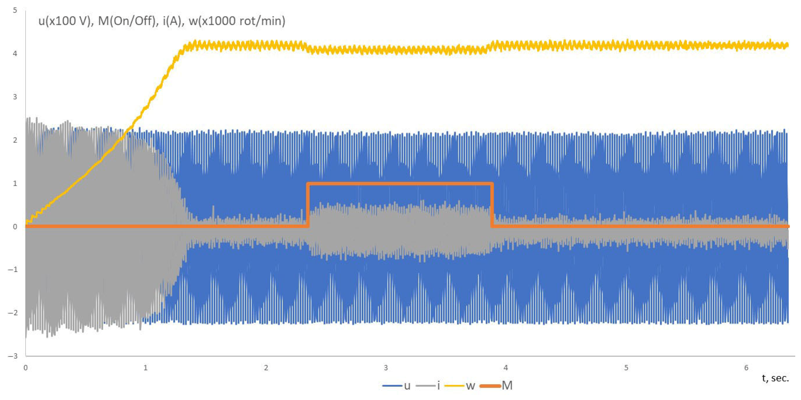
To construct a macromodel of a single-phase induction motor, a set of transient characteristics was selected to represent three key dynamic processes: motor start-up, stalling, and mechanical load shedding. The input variables of the macromodel were the supply voltage ${\mathit{U}}^{\left(\mathit{k}\right)}$ and the mechanical torque applied to the rotor ${\mathit{M}}^{\left(\mathit{k}\right)}$, while the output variables were the stator current ${\mathit{I}}^{\left(\mathit{k}\right)}$ and the rotor speed ${\mathit{\omega }}^{\left(\mathit{k}\right)}$, where $\mathit{k}=\overline{0,\mathit{N}}.$ Accordingly, for the macromodel of type (21), the following condition holds: $\mathbf{dim}{\overrightarrow{\mathit{v}}}^{\left(\mathit{k}\right)}=\mathit{dim}{\overrightarrow{\mathit{y}}}^{\left(\mathit{k}\right)}=\mathbf{2}$.

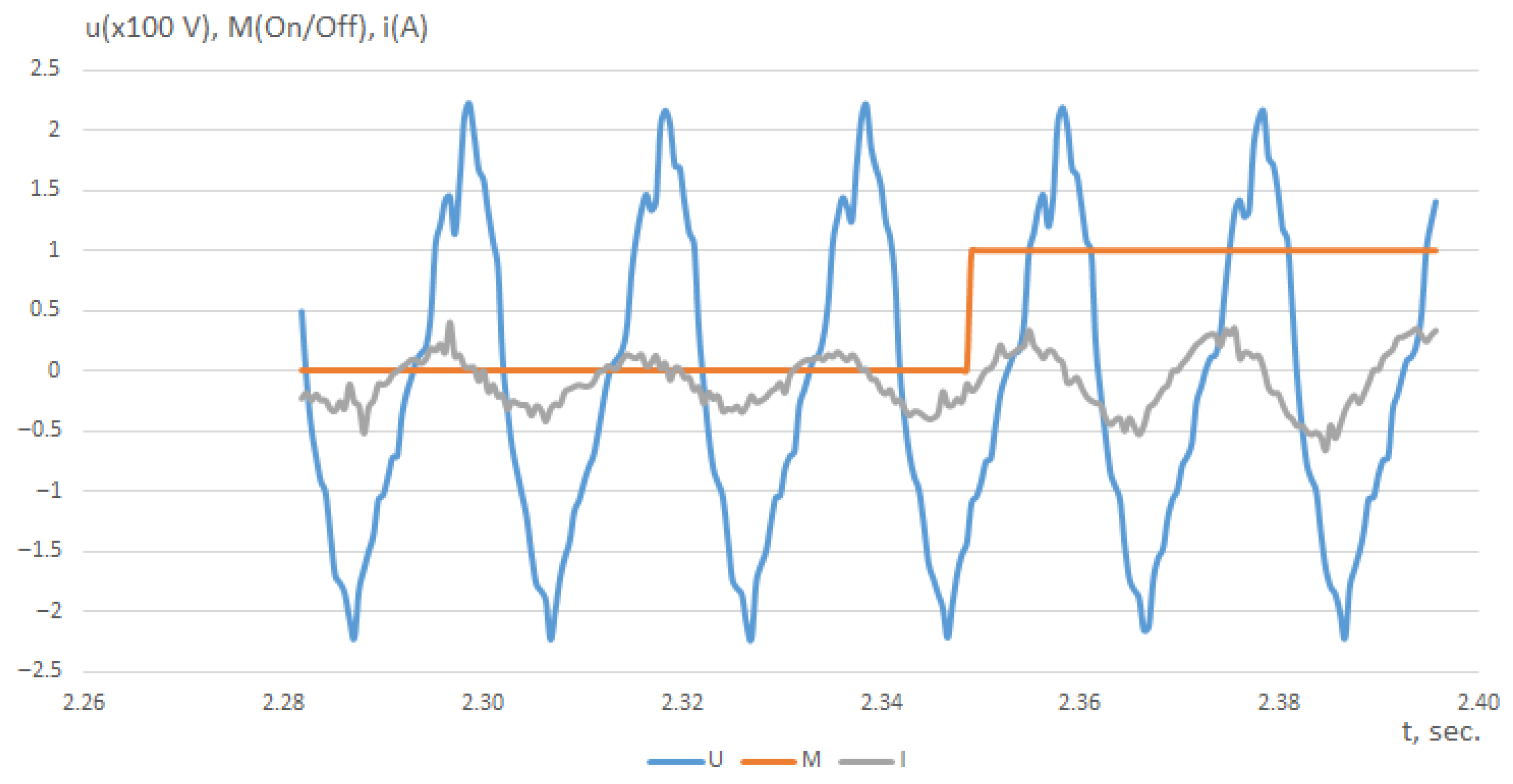
Figure 1 and Figure 2 present the overall view of the initial data set and a magnified fragment corresponding to the moment of load application.

Figure 1. Input data used for the construction of the macromodel.

Figure 2. Enlarged fragment of the input data used for macromodel construction at the moment of mechanical load increase. The rotor speed remains unchanged within this fragment and is therefore not shown.

A fragment of the discrete data used for the parametric identification of the macromodel is provided in Appendix A.

The structure of the macromodel was selected in accordance with the form presented in [34]:

$$\left\{\begin{array}{l}{\mathit{x}}_{\mathbf{1}}^{(\mathit{k}+\mathbf{1})}={\mathit{\lambda }}_{\mathbf{1}}·{\mathit{v}}_{\mathbf{1}}^{\left(\mathit{k}\right)}+{\mathit{\lambda }}_{\mathbf{2}}·{\mathit{x}}_{\mathbf{2}}^{\left(\mathit{k}\right)}·{\mathit{v}}_{\mathbf{1}}^{\left(\mathit{k}\right)}+{\mathit{\lambda }}_{\mathbf{3}}·{\left({\mathit{x}}_{\mathbf{1}}^{\left(\mathit{k}\right)}\right)}^{\mathbf{3}}+{\mathit{\lambda }}_{\mathbf{4}}·{\left({\mathit{x}}_{\mathbf{2}}^{\left(\mathit{k}\right)}\right)}^{\mathbf{3}}\\ {\mathit{x}}_{\mathbf{2}}^{(\mathit{k}+\mathbf{1})}={\mathit{\lambda }}_{\mathbf{5}}·{\mathit{x}}_{\mathbf{2}}^{\left(\mathit{k}\right)}+{\mathit{\lambda }}_{\mathbf{6}}·{\mathit{v}}_{\mathbf{2}}^{\left(\mathit{k}\right)}+{\mathit{\lambda }}_{\mathbf{7}}+{\mathit{\lambda }}_{\mathbf{8}}·{\mathit{x}}_{\mathbf{1}}^{\left(\mathit{k}\right)}·{\mathit{v}}_{\mathbf{1}}^{\left(\mathit{k}\right)}+{\mathit{\lambda }}_{\mathbf{9}}·{\left({\mathit{x}}_{\mathbf{1}}^{\left(\mathit{k}\right)}\right)}^{\mathbf{2}}·{\mathit{x}}_{\mathbf{2}}^{\left(\mathit{k}\right)}+{\mathit{\lambda }}_{\mathbf{10}}·{\mathit{x}}_{\mathbf{1}}^{\left(\mathit{k}\right)}·{\mathit{x}}_{\mathbf{2}}^{\left(\mathit{k}\right)}·{\mathit{v}}_{\mathbf{1}}^{\left(\mathit{k}\right)}\\ {\mathit{x}}_{\mathbf{3}}^{(\mathit{k}+\mathbf{1})}={\mathit{\lambda }}_{\mathbf{11}}·{\mathit{x}}_{\mathbf{3}}^{\left(\mathit{k}\right)}+{\mathit{\lambda }}_{\mathbf{12}}·{\mathit{v}}_{\mathbf{1}}^{\left(\mathit{k}\right)}+{\mathit{\lambda }}_{\mathbf{13}}·{\mathit{x}}_{\mathbf{2}}^{\left(\mathit{k}\right)}·{\mathit{v}}_{\mathbf{1}}^{\left(\mathit{k}\right)}+{\mathit{\lambda }}_{\mathbf{14}}·{\left({\mathit{x}}_{\mathbf{1}}^{\left(\mathit{k}\right)}\right)}^{\mathbf{2}}·{\mathit{v}}_{\mathbf{1}}^{\left(\mathit{k}\right)}+{\mathit{\lambda }}_{\mathbf{15}}·{\mathit{x}}_{\mathbf{2}}^{\left(\mathit{k}\right)}·{\mathit{v}}_{\mathbf{1}}^{\left(\mathit{k}\right)}·{\mathit{v}}_{\mathbf{2}}^{\left(\mathit{k}\right)}\\ {\mathit{y}}_{\mathbf{1}}^{(\mathit{k}+\mathbf{1})}={\mathit{\lambda }}_{\mathbf{16}}{·\mathit{x}}_{\mathbf{1}}^{(\mathit{k}+\mathbf{1})}+{{\mathit{\lambda }}_{\mathbf{17}}·\mathit{x}}_{\mathbf{3}}^{(\mathit{k}+\mathbf{1})}\\ {\mathit{y}}_{\mathbf{2}}^{(\mathit{k}+\mathbf{1})}={{\mathit{\lambda }}_{\mathbf{18}}·\mathit{x}}_{\mathbf{2}}^{(\mathit{k}+\mathbf{1})}\end{array}\right.$$

(22)

where ${{\mathit{v}}_{\mathbf{1}}^{\mathit{k}}=\mathit{U}}^{\left(\mathit{k}\right)};$ ${{\mathit{v}}_{\mathbf{2}}^{\mathit{k}}=\mathit{M}}^{\left(\mathit{k}\right)};$ ${\mathit{y}}_{\mathbf{1}}^{\left(\mathit{k}\right)}={\mathit{I}}^{\left(\mathit{k}\right)};{\mathit{y}}_{\mathbf{2}}^{\left(\mathit{k}\right)}={\mathit{\omega }}^{\left(\mathit{k}\right)};$ ${\mathit{\lambda }}_{\mathbf{1}}$, ${\mathit{\lambda }}_{\mathbf{5}}$, ${\mathit{\lambda }}_{\mathbf{6}}$, ${\mathit{\lambda }}_{\mathbf{11}}$, ${\mathit{\lambda }}_{\mathbf{12}}$, ${\mathit{\lambda }}_{\mathbf{16}}$, ${\mathit{\lambda }}_{\mathbf{17}}$, ${\mathit{\lambda }}_{\mathbf{18}}$ are non-zero elements of the matrices $\mathit{F},\mathit{G},\mathit{C};$ ${\mathit{\lambda }}_{\mathbf{2}}$, ${\mathit{\lambda }}_{\mathbf{3}}$, ${\mathit{\lambda }}_{\mathbf{4}}$, ${\mathit{\lambda }}_{\mathbf{7}}$, ${\mathit{\lambda }}_{\mathbf{8}}$, ${\mathit{\lambda }}_{\mathbf{9}}$, ${\mathit{\lambda }}_{\mathbf{10}}$, ${\mathit{\lambda }}_{\mathbf{13}}$, ${\mathit{\lambda }}_{\mathbf{14}}$, ${\mathit{\lambda }}_{\mathbf{15}}$ are coefficients of the nonlinear function $\overrightarrow{\mathit{\Phi }}\left(•\right); \mathit{k}=\overline{0,\mathit{N}}.$

The essence of parametric identification of macromodel (22) lies in finding such parameter values ${\mathit{\lambda }}_{\mathbf{1}}$, ${\mathit{\lambda }}_{\mathbf{2}}$, …, ${\mathit{\lambda }}_{\mathbf{18}}$, that the model most accurately reproduces the real behavior of the single-phase asynchronous motor under specified operating conditions. Thus, it is necessary to solve an optimization problem of type (3), where the components of the parameter vector $\overrightarrow{\mathit{\beta }}$ correspond to the model parameters ${\mathit{\lambda }}_{\mathbf{1}},{\mathit{\lambda }}_{\mathbf{2}},\dots ,{\mathit{\lambda }}_{\mathbf{18}}$.

Considering the number of system output signals (i.e., the dimension of ${\mathit{y}}_{\mathit{j}}^{\left(\mathit{k}\right)}$ and the number of discrete input and output values used for modeling), the objective function of the optimization problem takes the form:

$$\mathit{Q}({\mathit{\lambda }}_{\mathbf{1}}, {\mathit{\lambda }}_{\mathbf{2}}, \dots , {\mathit{\lambda }}_{\mathbf{18}})={\sum }_{\mathit{k}=\mathbf{1}}^{\mathit{N}}{\sum }_{\mathit{j}=\mathbf{1}}^{\mathbf{2}}{({\mathit{y}}_{\mathit{j}}^{\mathit{*}\left(\mathit{k}\right)}-{\mathit{y}}_{\mathit{j}}^{\left(\mathit{k}\right)})}^{\mathbf{2}},$$

(23)

where ${\mathit{y}}_{\mathit{j}}^{\mathit{*}\left(\mathit{k}\right)}$ denotes the $\mathit{k}$-th discrete value of the $\mathit{j}$-th real output signal, and ${\mathit{y}}_{\mathit{j}}^{\left(\mathit{k}\right)}$ is the corresponding value of the output signal obtained from model (22).

The solution of optimization problem (23) for the parametric identification of macromodel (22) using the directed cone method without adaptation of optimization parameters significantly exceeded the expected computational time under the selected simulation conditions. Therefore, the main focus was shifted to the use of three algorithms that incorporate parameter adaptation, namely: adaptation of the step size only (Algorithm 1), adaptation of both step size and hypercone angle (Algorithm 2), and proposed with the automatic implementation of the tunneling procedure (Algorithm 3).

The effectiveness of these algorithms was evaluated according to the following criteria: (i) the number of objective function evaluations required to reach the global minimum; (ii) the relative modeling accuracy; and (iii) the dynamics of progression across the hyperplane towards the global minimum. The global minimum was defined as the point beyond which further progression required a substantial increase in computational time. The relative modeling accuracy was defined as the current deviation from the absolute minimum of the objective function relative to its maximum possible value. The dynamics of progression were characterized by the dependence of the approach to the global minimum on the number of objective function evaluations.

Table 1 presents the first two performance indicators obtained for all three optimization algorithms.

Table 1. Results of the Evaluation of the Effectiveness of Optimization Algorithms.

Indicator	Algorithm 1 (Adaptation of the Step Size)	Algorithm 2 (Adaptation of Step Size and Hypercone Angle)	Algorithm 3 (Proposed)
Number of objective function evaluations	1,000,029	1,000,026	1,000,001
Relative accuracy of the macromodel, %	0.85	0.63	0.53

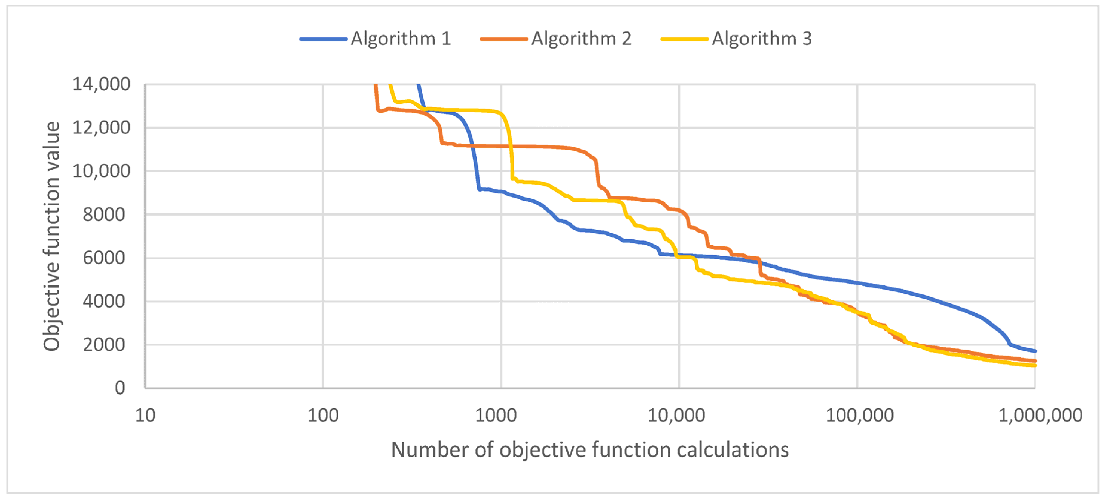
As can be seen from the presented results, the most effective algorithm for the considered modeling task is the one incorporating the tunneling procedure. It provides the highest modeling accuracy with the lowest computational cost. Conversely, the least effective among the applied algorithms was the one that included adaptation of the step size only. Figure 3 illustrates the dynamics of progression across the hyperplane toward the global minimum for the three algorithms under consideration.

Figure 3. Dynamics of progression across the hyperplane toward the global minimum.

As illustrated in the figure, during the initial stage of the optimization process, the algorithm with step-size adaptation only progresses toward the minimum point the fastest. However, in the final stage, its speed becomes lower compared to the other algorithms. Conversely, the algorithms with both step-size and hypercone angle adaptation, as well as with tunneling, are relatively slower at the beginning but faster at the final stage. As can be seen from Table 2, with the same number of objective function evaluations (approximately 1,000,000), the proposed algorithm provides a higher model accuracy, with a relative macromodel error of 0.53%, compared to Algorithm 1 (adaptation of the step size) with 0.85% and Algorithm 2 (adaptation of both the step size and hypercone angle) with 0.63%. The tunneling algorithm, in particular, is characterized by acceleration of the optimization process in certain regions, which indicates the selection of an optimal movement direction for the tunnel transition.

Table 2. Parameters of the single-phase asynchronous motor macromodel.

Parameter	Value	Parameter	Value
${\lambda }_1$	1.8005549	${\lambda }_{10}$	0.0021659
${\lambda }_2$	−0.3947988	${\lambda }_{11}$	0.9659041
${\lambda }_3$	−0.0368145	${\lambda }_{12}$	0.1000000
${\lambda }_4$	−0.0022357	${\lambda }_{13}$	−0.1850695
${\lambda }_5$	0.9983555	${\lambda }_{14}$	0.0067603
${\lambda }_6$	−0.0005524	${\lambda }_{15}$	0.0048879
${\lambda }_7$	0.0055210	${\lambda }_{16}$	1.0000000
${\lambda }_8$	−0.0012865	${\lambda }_{17}$	−0.8589651
${\lambda }_9$	−0.0018468	${\lambda }_{18}$	1.0000000

Since the highest accuracy for the considered modeling task is provided by the directed cone method with tunneling, the results of this algorithm are selected for the construction of the single-phase asynchronous motor macromodel. Table 2 presents the values of the objective function (23) arguments at the global minimum, which correspond to the parameters of macromodel (22) that most accurately reproduce the operating mode of the switched reluctance motor.

5. Conclusions

The complexity and diversity of electromechanical systems, as well as the need for their integration with other systems, motivate the development of universal and adequate mathematical models capable of being integrated into modern computer-aided modeling environments, such as MATLAB/Simulink R2023b. The problem addressed in this study relates directly to this issue, namely the modeling of electromechanical systems by developing a macromodel that integrates all elements of the system into a “black box.” The behavior of this black box is modeled based on observations of input and output signals, while the physical processes occurring inside the electromechanical system are disregarded. This approach eliminates the need to reconcile separate mathematical relationships describing the electrical and mechanical parts of the system. Consequently, the identification of the mathematical model of the electromechanical system is reduced to a nonlinear optimization problem. To solve this problem, the directed cone method is proposed and substantiated, which involves searching for the minimum of the objective function by stochastic movement across the hyperplane described by the optimization problem.

In applying this method, the main focus was placed on reducing computational complexity. Specifically, three improved algorithmic variants were proposed: (1) adaptation of the step size only; (2) adaptation of both the step size and the hypercone opening angle; and (3) the tunneling procedure.

The effectiveness of these algorithms was evaluated using the example of constructing a macromodel of a single-phase asynchronous motor. The performance criteria included the number of objective function evaluations until reaching the global minimum (computational time complexity), the relative modeling accuracy, and the dynamics of progression across the hyperplane toward the global minimum. The global minimum was defined as the point beyond which further progression requires a significant increase in computational effort. Relative accuracy was defined as the current deviation from the absolute minimum of the objective function relative to its maximum possible value. The dynamics of progression characterized the dependence of convergence toward the global minimum on the number of objective function evaluations.

The computational experiments demonstrated that the most effective algorithm was the tunneling variant, which achieved the highest modeling accuracy with fewer computational iterations. In contrast, the least effective algorithm was the one involving adaptation of the step size only.

Future research should expand the scope of analyzed electromechanical systems to establish the robustness of the proposed method with respect to model nonlinearity and to develop hybrid algorithms at different stages of the computational scheme of the method.

References

- Shynkarenko, V.F.; Shymanska, A.A.; Kotliarova, V.V. Modeling of Electromechanical Systems; Igor Sikorsky Kyiv Polytechnic Institute: Kyiv, Ukraine, 2019; Available online: https://ela.kpi.ua/handle/123456789/38793 (accessed on 29 September 2025). (In Ukrainian)
- Cieślik, S. Mathematical Modeling of the Dynamics of Linear Electrical Systems with Parallel Calculations. Energies 2021, 14, 2930. [Google Scholar] [CrossRef]
- Dubas, F.; Boughrara, K. Mathematical Models for the Design of Electrical Machines. Math. Comput. Appl. 2020, 25, 77. [Google Scholar] [CrossRef]
- Bu, W.; Li, J.; Lu, Y. Mathematical Modeling and Electromagnetic Characteristics Analysis of a Six-Phase Distributed Single-Winding BPMSM with 12 Slots and 2 Poles. Appl. Sci. 2025, 15, 2093. [Google Scholar] [CrossRef]
- Applications of Single Phase Induction Motor. GeeksforGeeks, 23 July 2025. Available online: https://www.geeksforgeeks.org/electrical-engineering/applications-of-single-phase-induction-motor/ (accessed on 30 October 2025).
- Baidak, Y. Single-Phase Motor of Hermetic Compressor Drive with Improved Performance Characteristics. Refrig. Eng. Technol. 2009, 118, 12–19. [Google Scholar]
- Baidak, Y. Mathematical Model of the Electric Motor of the Hermetic Compressor of the Refrigerating Appliance with a Single-Phase Winding. Refrig. Eng. Technol. 2009, 122, 6–15. [Google Scholar]
- Baidak, Y.; Smyk, V. Numerical Investigation of Refrigeration Machine Compressor Operation Considering Single-Phase Electric Motor Dynamic Characteristics. In Proceedings of the 10th International Conference on Compressors and Their Systems, IOP Conf. Ser. Mater. Sci. Eng. 2017, 232, 012081. [Google Scholar] [CrossRef]
- IEC 60034-30-1 ed1.0:2014; Rotating Electrical Machines—Part 30-1: Efficiency Classes of Line Operated AC Motors. International Electrotechnical Commission (IEC): Geneva, Switzerland, 2014.
- International Electrotechnical Commission (IEC). IEC 60050, Section 411-31: Rotating Machinery—General, IEV ref. 411-31-10: Induction Machine—An Asynchronous Machine of Which Only One Winding Is Energized; IEC: Geneva, Switzerland, 1990. [Google Scholar]
- Baidak, Y.; Vereitina, I. Asynchronous Electric Motor with Single-Phase Stator Winding. Autom. Technol. Bus.-Process. 2023, 15, 76–82. [Google Scholar] [CrossRef]
- Opolskiy, Y.V.; Vasyura, A.S. Modern Approaches to Increasing the Efficiency of Induction Motors. Optoelectron. Inf.-Power Technol. 2018, 35, 81–88. (In Ukrainian) [Google Scholar] [CrossRef]
- Klee, H.; Allen, R. Simulation of Dynamic Systems with MATLAB and Simulink; CRC Press: New York, NY, USA, 2011. [Google Scholar]
- Tkachuk, V.I.; Osidacz, Y.V. Modeling of electromechanical processes in an electric drive with a valve jet engine. Electr. Power Electromech. Syst. 1995, 288, 83–90. [Google Scholar]
- Czornyy, O.P.; Lugovoy, A.V.; Rolkin, A.Y.; Sysyuk, G.Y.; Sadovoy, O.V. Modeling of Electromechanical Systems. Kremenczuk, Ukraine. 2001. 410p (In Ukrainian). Available online: https://elprivod.nmu.org.ua/files/modeling/%D0%A7%D0%BE%D1%80%D0%BD%D0%B8%D0%B9_%D0%9C%D0%BE%D0%B4%D0%B5%D0%BB%D1%8E%D0%B2%D0%B0%D0%BD%D0%BD%D1%8F%20%D0%95%D0%9C%D0%A1.pdf (accessed on 20 May 2024).
- Stakhiv, P.G.; Kozak, Y.Y.; Hoholyuk, O.P. Discrete Modeling in Electrical Engineering and Related Fields; Lviv Polytechnic: Lviv, Ukraine, 2014. (In Ukrainian) [Google Scholar]
- Habash, R. Sustainability and Health in Intelligent Buildings; Woodhead Publishing: Cambridge, UK, 2022; Available online: https://shop.elsevier.com/books/sustainability-and-health-in-intelligent-buildings/habash/978-0-323-98826-1 (accessed on 20 May 2024).
- Ferreira, A.; Aphale, S.S. A Survey of Modeling and Control Techniques for Micro- and Nano-Electromechanical Systems. IEEE Trans. Syst. Man Cybern. Part C Appl. Rev. 2011, 41, 350–364. [Google Scholar] [CrossRef]
- Wee, H.S.H.; Ahmad, N.S. Review and Comparative Analysis of System Identification Methods for Perturbed Motorized Systems. Comput. Model. Eng. Sci. 2025, 143, 1301–1354. [Google Scholar] [CrossRef]
- Dri, E.; Peretti, G.; Romero, E. Fault Detection in Configurable Switched-Capacitor Filters Using Transient Analysis and Dynamic Time Warping. Analog Integr. Circuits Signal Process. 2021, 108, 1–14. [Google Scholar] [CrossRef]
- Oh, J.; Yu, Y.S. Macro-Modeling for N-Type Feedback Field-Effect Transistor for Circuit Simulation. Micromachines 2021, 12, 1174. [Google Scholar] [CrossRef] [PubMed]
- Amick, B.W.; Gauthier, C.R.; Liu, D. Macro-Modeling Concepts for the Chip Electrical Interface. In Proceedings of the 2002 Design Automation Conference (DAC 2002), New Orleans, LA, USA, 10–14 June 2002; Available online: https://www.cs.york.ac.uk/rts/docs/SIGDA-Compendium-1994-2004/papers/2002/dac02/pdffiles/27_3.pdf (accessed on 10 May 2024).
- Kvatinsky, S.; Friedman, E.G.; Kolodny, A.; Schächter, L. Power Grid Analysis Based on a Macro Circuit Model. In Proceedings of the IEEE 26th Convention of Electrical and Electronics Engineers in Israel, Eilat, Israel, 17–20 November 2010; Available online: https://asic2.group/wp-content/uploads/2017/06/kvatinsky.pdf (accessed on 15 June 2024).
- Sass, L. Symbolic Modeling of Electromechanical Multibody Systems. Ph.D. Thesis, Université catholique de Louvain, Louvain, Belgium, 2004. Available online: https://dial.uclouvain.be/pr/boreal/object/boreal:5194/datastream/PDF_01/view (accessed on 25 July 2024).
- Tan, D.; Shi, C. Efficient Approximation of Symbolic Expressions for Analog Behavioral Modeling and Analysis. IEEE Trans. Comput.-Aided Des. Integr. Circuits Syst. 2004, 23, 907–918. [Google Scholar] [CrossRef]
- Lin, Y.; Li, Y.; Madhusudan, M.; Sapatnekar, S.S.; Harjani, R.; Hu, J. MMM: Machine Learning-Based Macro-Modeling for Linear Analog ICs and ADC/DACs. IEEE Trans. Comput.-Aided Des. Integr. Circuits Syst. 2024, 43, 4740–4752. [Google Scholar] [CrossRef]
- Pandit, S. Nano-Scale CMOS Analog Circuits: Models and CAD Techniques for High-Level Design; CRC Press: Boca Raton, FL, USA, 2014. [Google Scholar] [CrossRef]
- Petrenko, A. Macromodels of Micro-ElectroMechanical Systems (MEMS). In Microelectromechanical Systems and Devices; IntechOpen: London, UK, 2012; pp. 155–190. Available online: https://cdn.intechopen.com/pdfs/33594/InTech-Macromodels_of_micro_electro_mechanical_systems_mems_.pdf (accessed on 20 December 2024).
- Romansky, R. An Approach for Mathematical Modeling and Investigation of Computer Processes at a Macro Level. Mathematics 2020, 8, 1838. [Google Scholar] [CrossRef]
- Arrillaga, J.; Watson, N. Power Systems Electromagnetic Transients Simulation; The Institution of Electrical Engineers: London, UK, 2003; 421p. [Google Scholar]
- Zadeh, L.A.; Desoer, C.A. Linear System Theory: The State Space Approach; Courier Dover Publications: Mineola, NY, USA, 2008. [Google Scholar]
- Viola, C.; Pavesi, D.; Weng, L.; Gobat, G.; Maspero, F.; Zega, V. Microelectromechanical System Resonant Devices: A Guide for Design, Modeling and Testing. Micromachines 2024, 15, 1461. [Google Scholar] [CrossRef]
- Santana, N.H.B.; Yahyaoui, I.; Oliveira, F.D.C.; Amorim, A.E.A.; Simonetti, D.S.L.; Rocha, H.R.O. Dynamic to Static Model Comparison and Hybrid Metaheuristic Optimization in Induction Motor Parameter Estimation. Electronics 2025, 14, 524. [Google Scholar] [CrossRef]
- Ljung, L. System Identification Toolbox for Use with MATLAB, Version 6; The MathWorks, Inc.: Natick, MA, USA, 2003. [Google Scholar]
- Kiss, G.R.; Horváth, M.; Szánthó, Z. MATLAB Simulink-Based Modelling and Performance Analysis of District Heating Substations for Renewable Energy Integration. Energies 2025, 18, 2370. [Google Scholar] [CrossRef]
- Naqvi, S.F.A. Mathematical Modeling & MATLAB Simulation of STATCOM Based Profile Controller for Self Excited Induction Generator. In Proceedings of the 2023 IEEE 12th International Conference on Communication Systems and Network Technologies (CSNT), Bhopal, India, 8–9 April 2023; pp. 975–982. [Google Scholar] [CrossRef]
- Silvestrov, A.; Ostroverkhov, M.; Spinul, L.; Serdyuk, A.; Falchenko, M. Structural and parametric identification of mathematical models of control objects based on the principle of rational complication. In Proceedings of the 2022 IEEE 3rd KhPI Week on Advanced Technology (KhPIWeek), Kharkiv, Ukraine, 3–7 October 2022; pp. 1–4. [Google Scholar] [CrossRef]
- Lasdon, L.S.; Fox, R.L.; Ratner, M.W. Nonlinear optimization using the generalized reduced gradient method. RAIRO-Oper. Res.-Rech. Opérationnelle 1974, 8, 73–103. Available online: http://eudml.org/doc/104604 (accessed on 22 December 2024). [CrossRef]
- Rastrigin, L.A. Random Search in Optimization Problems for Multiparameter Systems; Air Force Systems Command, Foreign Technology Division: Wright-Patterson AFB, OH, USA, 1967; (English translation of Sluchainyi Poisk v Zadachakh Optimizatsii Mnogoparameticheskikh Sistem, Akademiia Nauk Latviiskoi SSR: Riga, USSR, 1965). [Google Scholar]
- White, R.C. A Survey of Random Methods for Parameter Optimization. EUT Report E 70-E-16; Technische Hogeschool Eindhoven: Eindhoven, The Netherlands, 1970; Available online: https://pure.tue.nl/ws/portalfiles/portal/4396577/7101031.pdf (accessed on 23 January 2024).
- Stakhiv, P.; Hoholyuk, O.; Hamola, O.; Melnyk, B.; Maday, V.; Melnyk, N. Application of the Rastrygin’s Method in Modeling of Complex Electrical Systems. In Proceedings of the 2023 24th International Conference on Computational Problems of Electrical Engineering (CPEE), Grybów, Poland, 10–13 September 2023; IEEE: Piscataway, NJ, USA, 2023; pp. 1–6. [Google Scholar] [CrossRef]
- Duong, T.-T.; Pham, D.N.; Sattar, A. A study of local minimum avoidance heuristics for SAT. In Proceedings of the ECAI 2012, Frontiers in Artificial Intelligence and Applications, Montpellier, France, 27–31 August 2012; IOS Press: Amsterdam, The Netherlands, 2012; Volume 242, pp. 300–305. [Google Scholar]
- Bukashkin, S.A. Numerical Methods for Optimal Synthesis of Linear and Non-Linear Recursive Electronic Circuits. Ph.D. Thesis, Riga Aeronautical Institute, Riga, Latvia, 1989; 516p. [Google Scholar]
- Dzhala, V. Statistical global optimization algorithm with search step adaptation. Probl. Control Inform. 1997, 2, 90–94. [Google Scholar] [CrossRef]
- Kozak, Y.Y. Modification of Rastrigin’s guide cone method. Electron. Commun. Themat. Issue Probl. Phys. Biomed. Electron. 1997, 2 Pt 1, 424. (In Ukrainian) [Google Scholar]
- Stakhiv, P.G.; Kozak, Y.Y.; Selepyna, Y.R. Improving the optimization algorithm for identifying parameters of macromodels of electromechanical systems. Electr. Power Electromech. Syst. 2010, 666, 98–102. (In Ukrainian) [Google Scholar]
- Dyvak, M.; Melnyk, A.; Rot, A.; Hernes, M.; Pukas, A. Ontology of Mathematical Modeling Based on Interval Data. Complexity 2022, 2022, 8062969. [Google Scholar] [CrossRef]
- Dyvak, M.; Manzhula, V.; Melnyk, A.; Rusyn, B.; Spivak, I. Modeling the Efficiency of Biogas Plants by Using an Interval Data Analysis Method. Energies 2024, 17, 3537. [Google Scholar] [CrossRef]
- Tkachuk, V.; Klytta, M. Electronic commutator with parallel capacity storage for switched reluctance motor. Comput. Probl. Electr. Eng. 2011, 1, 107–112. Available online: https://ena.lpnu.ua:8443/server/api/core/bitstreams/17b751c9-d8a0-423e-84bf-95cdc024c503/content (accessed on 29 September 2025).
- Stakhiv, P.; Melnyk, B.; Hoholyuk, O.; Trokhaniak, S. Application of parallel computing technology for modelling complex dynamic objects. Comput. Probl. Electr. Eng. 2024, 14, 30–35. [Google Scholar] [CrossRef]
Disclaimer/Publisher’s Note: The statements, opinions and data contained in all publications are solely those of the individual author(s) and contributor(s) and not of MDPI and/or the editor(s). MDPI and/or the editor(s) disclaim responsibility for any injury to people or property resulting from any ideas, methods, instructions or products referred to in the content. |
© 2025 by the authors. Licensee MDPI, Basel, Switzerland. This article is an open access article distributed under the terms and conditions of the Creative Commons Attribution (CC BY) license (https://creativecommons.org/licenses/by/4.0/).