Analysis of Instantaneous Energy Consumption and Recuperation in Electric Buses During SORT Tests Using Linear and Neural Network Models

Abstract

With the growing deployment of electric buses (e-buses), accurate energy use modelling has become essential for fleet optimisation and operational planning. Using the SORT methodology, this study analyses instantaneous energy consumption and recuperation (IECR). Three vehicle configurations were tested (one battery with pantograph, four batteries, and eight batteries), each with ten repeatable runs. Four approaches were compared: a baseline linear regression, an extended linear model (ELM) due to the state, a feed-forward neural network, and a recurrent neural network (RNN). The extended linear model achieved a determination coefficient of R² = 0.9124 (residual standard deviation 4.26) compared with R² = 0.7859 for the baseline, while the determination coefficient for the RNN is 0.9343, and the RNN provided the highest accuracy on the test set (the correlation coefficient between real and predicted values is 0.9666). The results confirm the dominant influence of speed and acceleration on IECR and show that battery configuration mainly affects consumption during acceleration. Literature-consistent findings indicate that regenerative systems can recover 25–51% of braking energy, with advanced control methods further improving recovery. Despite non-normality and temporal dependence of residuals, the state-aware linear model remains interpretable and competitive, whereas recurrent networks offer superior fidelity. These results support real-time energy management, charging optimisation, and reliable range prediction for electric buses in urban public transport.

1. Introduction

With the rising prevalence of electric buses, modelling their energy efficiency emerges as a critical challenge, supporting effective operational planning and fleet optimisation. Energy consumption in these vehicles is influenced by multiple aspects, including driving dynamics, operating conditions, terrain topography, and vehicle technical parameters. Accurate modelling allows improving energy efficiency, optimising charging strategies, and extending battery life. Analysing energy consumption in electric buses can support the optimisation of energy management strategies and improve the efficiency of transportation systems. Using statistical methods, machine learning algorithms, and physical modelling enables precise energy consumption forecasting and the adjustment of operational strategies [1]. In urban conditions, eco-driving practices have been shown to reduce vehicle energy use, supporting operational goals in public transport [2]. Additionally, vehicle configuration has been shown to shape energy demand; a comparative study of short versus long city buses reported systematic differences in energy consumption with implications for e-mobility planning [3].

For public transport applications, the Standardised On-Road Test (SORT) methodology serves as an important tool to assess vehicle energy efficiency in quasi-real operating environments. It involves three driving cycles, SORT 1 (intensive urban), SORT 2 (moderate urban), and SORT 3 (suburban), each characterised by differences in speed profiles, stop patterns, and passenger loads [4,5]. Unlike previous test cycles (e.g., ESC, ETC), the SORT methodology evaluates the entire vehicle, not just the engine, allowing for accurate energy consumption comparisons and the effectiveness of recuperation systems. The results of these tests are widely used in tenders for rolling stock purchases and operational optimisation processes. Within such evaluations, broader sustainability indicators for surface public transport should also be considered [6].

Predictive models have assumed greater importance for public transport in recent years, contributing to real-time optimisation of energy efficiency. Models based on predictive control (MPC) can adapt energy management strategies to current road conditions, battery status, and predicted driving speeds, reducing energy consumption by up to several per cent compared to traditional methods [7,8,9,10,11]. Modern modelling approaches increasingly employ machine and deep learning techniques, including long short-term memory (LSTM) and bidirectional LSTM (BiLSTM), which enhance predictive accuracy and allow adaptation to dynamic operating conditions. Predictive models can also account for component ageing, translating into extended battery life and reduced fleet maintenance costs [12].

A key element in improving the efficiency of electric buses is the strategy of energy recuperation during braking. Supercapacitors, flywheels, or flow batteries offer high cycle life and fast energy exchange, making them promising for energy storage in SORT-based systems. These findings align with emerging research on dynamic energy transfer at intersections, which leverages regenerative braking to optimise system-wide energy recovery [13]. Modern energy recovery systems can recover from 25 to as much as 51% of braking energy. The use of advanced control methods, such as threshold logic, fuzzy control, or genetic algorithms, can increase this recovery by another dozen or so per cent compared to basic strategies [14,15]. Optimising energy recuperation translates into reduced overall energy consumption, extended vehicle range, and better battery protection, especially when integrated with hybrid energy storage systems.

Despite progress, the literature indicates significant research gaps in analysing instantaneous energy consumption in electric buses during SORT tests. There is a lack of comprehensive studies combining instantaneous energy consumption profiles with linear and non-linear models in real-world operating scenarios. Previous work shows that non-linear models, such as neural networks, better represent complex relationships than linear models, but they require the inclusion of additional variables, time delays, and environmental factors to improve forecast accuracy [4,16].

This paper analyses electric buses’ instantaneous energy consumption and recuperation (IECR) based on SORT tests. The study included vehicles equipped with one battery with a pantograph, four batteries, and eight batteries, each of which underwent ten test runs. The study applied linear regression together with artificial neural networks to capture how driving parameters influence energy consumption. The obtained results enabled the assessment of the effect of speed and acceleration on instantaneous energy consumption and recuperation, as well as the analysis of the impact of battery configuration on vehicle energy efficiency. These results can provide a basis for further optimising public transport systems through advanced energy management strategies and precise range forecasting of electric buses in urban environments.

2. Literature Review

Modelling energy consumption in electric bus drive systems is key to optimising public transport. Abdelaty et al. [17] and Abdelaty & Mohamed [18] demonstrated the high effectiveness of machine learning models, such as neural networks, in predicting energy consumption. Li et al. [1] proposed a model combining physical and historical data, which allows for more accurate predictions. Energy consumption modelling in electric vehicles has been widely studied in the scientific literature. Kozłowski et al. [19] indicated that vehicle speed, acceleration, and the transformations of these characteristics are key factors determining energy consumption in electric vehicles. These studies demonstrated that dynamic speed changes can significantly affect energy efficiency, which is particularly important in urban conditions. Further research by Kozłowski et al. [4] focused on analysing instantaneous energy consumption and the recuperation (IECR) process, drawing on SORT test measurements. In parallel to consumption modelling, EV routing studies integrate battery range and charger topology; GA-based methods are a common and effective option [20]. These results confirm the significance of efficient energy control strategies, especially in optimising energy recovery systems.

Dabčević et al. [21] developed a model to analyse bus trip data, considering average speed and distance travelled. Vepsäläinen et al. [22] highlighted the computational efficiency of predictive methods, which is crucial for applications in real-world operating conditions. Kozłowski et al. [19] analysed the availability of technical systems using a semi-Markov model, which allows for considering random periods of idleness and operation of electric vehicles. Applying this model in public transport analysis can be crucial for predicting the reliability of electric buses and their effective management. At the system level, initiatives such as Bus Rapid Transit (BRT) have proven effective in improving the efficiency and sustainability of bus operations, thereby facilitating the integration of predictive modelling with urban mobility planning [23]. In addition, Kozłowski et al. [4] investigated instantaneous energy use and the recuperation process using data obtained from SORT trials. These results confirm the importance of effective energy management, especially in optimising energy recovery systems. In the context of predictive methods, Kłosowski et al. [24] applied LSTM neural networks to monitor complex industrial systems, demonstrating the potential application of this technology in modelling energy consumption in electric buses. Furthermore, Pawlik et al. [25] demonstrated the effectiveness of artificial neural networks in diagnosing machines operating under variable conditions, suggesting the possibility of using similar techniques in the operational analysis of electric vehicles.

An important issue in energy consumption analysis is obtaining measurement data. Electric vehicles use, among others, on-board diagnosis (OBD) systems, the control area network (CAN) bus, on-board sensors, and external data loggers. OBD-II enables real-time acquisition of parameters such as speed, battery current and voltage, and state of charge (SOC), which allows for conducting research in real-world conditions [26,27,28,29]. Access to the CAN bus enables the recording of detailed data from the drivetrain and auxiliary systems, characterised by a higher frequency of measurements [30]. On-board sensors allow for direct measurement of current, voltage, speed, acceleration, and environmental conditions [29,31]. Data loggers enable long-term recording of parameters from multiple sources, integrating data from GPS and environmental sensors, which is particularly useful in predictive models [28,30,31].

Energy consumption models can be regression-based or based on neural networks. Linear regression models are interpretable and straightforward but often fail to model non-linear dependencies [32,33,34]. Neural networks are good at modelling non-linearities [35,36], while recurrent architectures (RNN, LSTM, GRU) enable the representation of temporal dependencies and achieve higher forecast accuracy [37,38,39].

Speed, acceleration, vehicle mass, and route profile primarily influence instantaneous energy consumption. Higher speeds and rapid accelerations increase energy consumption due to increased aerodynamic drag and power requirements (Suarez et al., 2022; Skuza et al., 2024 [40,41]). Higher mass—due to the number of passengers or battery configuration—increases consumption, especially on hills [42]. Route configuration, number of stops, and traffic density also play a significant role [43,44].

Recovering electrical energy during braking is one of the key mechanisms for improving efficiency. Chidambaram et al. [45] show that a high recuperation level at low charging currents benefits battery life. The braking strategy significantly impacts energy balance—aggressive methods allow for the recovery of more energy at the expense of faster cell degradation. In contrast, gentle methods are more beneficial for battery durability [46]. Additionally, advanced control strategies, such as fuzzy control or hybrid systems with supercapacitors, can increase energy recovery efficiency by up to 15% [47,48]. The number of batteries in an electric vehicle can affect its energy consumption, mainly due to increased weight.

The literature on braking energy recovery shows that the recovery strategy affects the efficiency of energy recovery. An aggressive strategy enables the recovery of a larger amount of electrical energy during braking, which translates into an increase in range. Although a gentle method produces less electrical energy, it may be more convenient for the vehicle driver and drivetrain [49]. Comparative assessment of regenerative braking performance in a fully electric car was performed. An aggressive method causes a higher current load on the battery, which may cause its faster degradation and shorten its lifespan. In turn, a gentle method is better for battery longevity. Driving style also affects the speed of battery regeneration and energy recovery efficiency from braking [50]. Another factor influencing energy consumption is the configuration of the battery system [42]. An increase in the number of batteries means an increase in weight. This relationship is directly proportional—the more batteries, the greater the weight. An increase in weight also has an impact on increasing rolling resistance. Optimising the weight and arrangement of batteries affects the vehicle’s energy efficiency and maximises range [49]. The number of batteries also increases the range. For most users, the optimal range is 350–480 km. Further increase in battery capacity becomes less effective [42,49].

Comparisons of laboratory test results (e.g., SORT) with data from real-world routes indicate significant differences resulting from the influence of traffic conditions, driver behaviour, and environmental factors [51]. Therefore, combining both data sources to obtain reliable models is recommended.

Energy efficiency assessment requires the use of statistical analysis methods and model validation methods [52,53]. It is important to use visual inspection of residual plots and error measures (RMSE, MAE, correlation coefficient) to assess model fit comprehensively.

Environmental factors also influence energy consumption. Low temperatures increase energy demand due to increased heating consumption and reduced battery efficiency, which can increase consumption by up to 35–50% in winter conditions [54,55]. High temperatures also increase consumption due to air conditioning [36]. Unfavourable weather conditions, such as wind, rain, or snow, further reduce efficiency [56,57].

3. Materials and Methods

Electric buses’ IECR were analysed during the SORT test. The study included three vehicle configurations as follows:

• Electric bus with one battery and fitted with a pantograph;
• Electric bus with four batteries;
• Electric bus with eight batteries.

The tests were conducted on standard 12-metre low-floor city buses in three battery configurations: one pack with a pantograph (nominal capacity 72.4 kWh), four packs (nominal capacity 290 kWh), and eight packs (nominal capacity 579 kWh). All buses were loaded to their permissible gross vehicle weight (approx. 18,000 kg) to ensure comparable test conditions.

Ten test runs were conducted for each variant. The analysis sought to identify the effect of battery number on energy consumption and recuperation while driving and to assess the dependence of IECR on speed and driving dynamics (acceleration). Modelling was conducted using the following:

• A linear model considering the contrast describing the system state (acceleration, braking, steady driving, stopping);
• A complex linear model considering the states of the system;
• Artificial neural network;
• Recurrent neural network.

Linear models, despite the generally non-linear nature of the dependence of IECR on velocity and acceleration, linearly use variables and their transformations in estimating the effect on IECR.

3.1. Measuring Equipment

The following devices were used for the measurements:

• Yokogawa WT-1806 power analyser (Musashino, Japan);
• APPA 32 current clamp (Shin-Tien, Taiwan);
• LAB-EL LB-702 thermohygrobarometer—measuring probe No. 1371 and reading panel No. 1073 (Łódź, Poland);
• CFM Master anemometer model 8901; serial number 8809870 (Frankfurt, Germany);
• CORSYS-DATRON measuring head type L-400 serial no. 41434 (Darmstadt, Germany);
• DINI ARGEO non-automatic electronic scale type WWSD6T; serial number 01001852335 (Modena, Italy).

Speed was measured using a DATRON optical head, synchronised with energy consumption and recovery measurements. The measurement system displayed a speed profile to the driver by the SORT cycle requirements, ensuring high repeatability of runs.

Current clamps were connected at points in the vehicle’s high-voltage system (PowerBox, main HV connectors), allowing for the recording of current flow during acceleration, braking, constant speed driving, and standstill. These points are illustrated in the measurement system diagrams. Voltage measurements were performed at dedicated points in the electrical system, enabling battery performance monitoring during operation and charging.

3.2. Measurement Location and Conditions

The tests were carried out on Road No. 56 near Stary Jasiniec. The measurement section, 2100 m in length, featured a maximum gradient of 0.35% and was located at an elevation of 98 m above sea level, with a smooth road surface. During the trials, atmospheric conditions remained stable, with wind speeds along the route between 0.40 and 0.54 m/s, air temperature ranging from 5.2 to 4.7 °C, relative humidity of 60.4–65.3%, and pressure between 1005.1 and 1005.3 hPa.

3.3. SORT Test Procedure

The SORT developed by UITP includes three variants as follows:

• SORT 1—intense city traffic (average speed approx. 12 km/h, 6–8 stops/km, stop time up to 35% of driving time);
• SORT 2—moderate city traffic (approx. 18 km/h, 3–5 stops/km, standing still approx. 20% of the time);
• SORT 3—suburban route (approx. 25 km/h, 1–2 stops/km, stops approx. 10% of the time).

The tests maintained the full load per its permissible gross vehicle weight. Multiple iterations were performed for each vehicle variant to obtain data with minimal deviation from the reference profile. The results were measured in kWh/km, recording energy consumption and recuperation during braking.

3.4. Data Analysis

The collected data were time-synchronised, and the dependence of IECR on vehicle speed, acceleration, and driving states was then modelled. The effect of battery number on energy consumption and recovery characteristics was considered. The models were assessed for fit and predictive ability.

4. Research Tools

This section presents the research tools applied in the study, including both statistical and computational methods. The aim was to evaluate the instantaneous energy consumption and recuperation under different operational conditions of the buses. The methods range from linear models, which provide a simplified view of the system, to advanced neural networks, which enable capturing complex non-linear dependencies. The following subsections describe the tools in detail.

4.1. Linear Model

Let $\{\left(IEC{R}_t,b_t,v_t,a_t\right){\}}_{1\le t\le n}$ denote a dataset, where $IC{E}_t$ denotes the energy consumed during 1 s of measurement (Wh), $v_t$ is the average vehicle speed ($\mathrm{k}\mathrm{m}/\mathrm{h}$), $a_t \mathrm{i}\mathrm{s}$ acceleration $(\mathrm{m}/{\mathrm{s}}^2)$, and $b_t\in \{1\mathrm{b},4\mathrm{b},8\mathrm{b}\}$ is the number of batteries installed in the bus. Since the variable describing the number of batteries is a qualitative variable, we choose 1 battery with a pantograph as the reference level. Speed and acceleration are the main factors influencing the amount of energy consumed and recovered, which is why four vehicle states were distinguished. Therefore, the vehicle’s journey is described by its stay in the states. We distinguish between four states: $A$—acceleration, $B$—braking, $D$—driving, and $S$—stop. Therefore, a function $\varphi \left(v,a\right):{\mathbb{R}}^{+}\times \mathbb{R}\to \{A,B,D,S\}$ of the form was constructed

$$\left(v,a\right)=\left\{\begin{array}{ll}S,& v<v_{min},\\ A,& v\ge v_{min} \mathrm{and} a>a_{min},\\ B,& v\ge v_{min} \mathrm{and} a<-{\alpha }_{min},\\ D,& \mathrm{other}.\end{array}\right.$$

The value $v_{min}$ denotes the minimum vehicle speed below which we assume that the bus is in state S, and ${\alpha }_{min}$ is the absolute value of acceleration. If the bus speed exceeds $v_{min}$ and acceleration is below the level—${\alpha }_{min}$, we assume that the vehicle is in state B (braking). If the speed exceeds $v_{min}$ and acceleration exceeds ${\alpha }_{min}$, we assume that the vehicle is in state A (acceleration). When the speed exceeds $v_{min}$ and the absolute value of acceleration is below ${\alpha }_{min}$, then we accept that the vehicle is in state D (driving).

To check the influence of the number of batteries installed in the bus, speed, and acceleration on the IECR at each moment $t$, $1\le t\le n$, we consider a linear model as follows:

$$\begin{array}{c}IEC{R}_t={\theta }_0+{\theta }_1{v}_t+{\theta }_2{a}_t+{\theta }_3{a}_t^2+{\theta }_4{v}_t{a}_t+{\theta }_5{I}_t^{\varphi }\left(B\right)+{\theta }_6{I}_t^{\varphi }\left(D\right)+\\ {\theta }_7{I}_t^{\varphi }\left(S\right)+{\theta }_8{I}_t^b\left(4\mathrm{b}\right)+{\theta }_9{I}_t^b\left(8\mathrm{b}\right)+{\epsilon }_t,\end{array}$$

(1)

where the predictors $v_t,a_t,a_t^2,v_t{a}_t$ linearly influence the size of IECR, and

$$I_t^b\left(k\right)=\left\{\begin{array}{ll}1,& b_t=k,\\ 0,& b_t\ne k\end{array}\right., I_t^{\varphi }\left(s\right)=\left\{\begin{array}{ll}1,& \varphi \left(v_t,a_t\right)=s,\\ 0,& \varphi \left(v_t,a_t\right)\ne s\end{array}\right.$$

for $k\mid in\in \{4\mathrm{b},8\mathrm{b}\}$ and $s\in \{A,B,D,S\}$, while external factors’ influence is represented by a random variable with a normal distribution $N\left(0,{\sigma }^2\right)$.

Parameter ${\theta }_0$ corresponds to the intercept in the model for the case of a bus with one battery and is in a state of acceleration, and ${\theta }_5$ is responsible for the change in IECR for the state of braking. ${\theta }_6$ is the state of driving, ${\theta }_7$ is the for the state of stop, ${\theta }_8$ is the change in IECR for a bus with four batteries, and ${\theta }_9$ for a bus with eight batteries. The remaining parameters in model (1) are responsible for the vehicle dynamics influence on the instantaneous energy consumption. Therefore, for the training set, we solve the problem

$$\begin{array}{c}\underset{\left({\theta }_0,{\theta }_1,\dots ,{\theta }_9\right)\in {\mathbb{R}}^{10}}{\mathrm{m}\mathrm{i}\mathrm{n}}{\displaystyle \sum _{t=1}^n}\left(IEC{R}_t-{\theta }_0-{\theta }_1{v}_t-{\theta }_2{a}_t-{\theta }_3{a}_t^2-{\theta }_4{v}_t{a}_t-{\theta }_5{I}_t^{\varphi }\left(B\right)-\right.\\ {\left.{\theta }_6{I}_t^{\varphi }\left(D\right)-{\theta }_7{I}_t^{\varphi }\left(S\right)-{\theta }_8{I}_t^b\left(4\mathrm{b}\right)-{\theta }_9{I}_t^b\left(8\mathrm{b}\right)\right)}^2\end{array}$$

(2)

The squares method is used to estimate the structural parameters ${\theta }_0,{\theta }_1,\dots ,{\theta }_9$ [58,59]. IECR predictions estimate

$$\begin{array}{c}{\widehat{IECR}}_t={\widehat{\theta }}_0+{\widehat{\theta }}_1{v}_t+{\widehat{\theta }}_2{a}_t+{\widehat{\theta }}_3{a}_t^2+{\widehat{\theta }}_4{v}_t{a}_t+{\widehat{\theta }}_5{I}_t^{\varphi }\left(B\right)+{\widehat{\theta }}_6{I}_t^{\varphi }\left(D\right)+\\ {\widehat{\theta }}_7{I}_t^{\varphi }\left(S\right)+{\widehat{\theta }}_8{I}_t^b\left(4\mathrm{b}\right)+{\widehat{\theta }}_9{I}_t^b\left(8\mathrm{b}\right)+{\epsilon }_t,\end{array}$$

(3)

4.2. Extended Linear Model Concerning States

Since we use $\varphi \left(v,a\right):{\mathbb{R}}^{+}\times \mathbb{R}\to \{A,B,D,S\}$ to determine the vehicle states, we analyzed the linear dependence of battery quantity, speed, and acceleration, as well as the transformation of these variables for each state (acceleration, braking, driving) and the influence of battery quantity on the stop state. The extended linear model (ELM) concerning states is presented as follows:

$$IEC{R}_t=\sum _{j\in \{A,B,D,S\}}{I}_t^{\varphi }\left(j\right)f_j\left({\Theta }_j,v_t,a_t\right)+{\epsilon }_t$$

(4)

$$f_A\left({\Theta }_A,v_t,a_t\right)={\theta }_0^A+{\theta }_1^A{I}_t^b\left(4\mathrm{b}\right)+{\theta }_2^A{I}_t^b\left(8\mathrm{b}\right)+{\theta }_3^A{v}_t+{\theta }_4^A{a}_t+{\theta }_5^A{a}_t^2+{\theta }_6^A{v}_t{a}_t,$$

(5)

$$f_B\left({\Theta }_B,v_t,a_t\right)={\theta }_0^B+{\theta }_1^B{I}_t^b\left(4\mathrm{b}\right)+{\theta }_2^B{I}_t^b\left(8\mathrm{b}\right)+{\theta }_3^B{v}_t+{\theta }_4^B{a}_t+{\theta }_5^B{a}_t^2+{\theta }_6^B{v}_t{a}_t,$$

(6)

$$f_D\left({\Theta }_D,v_t,a_t\right)={\theta }_0^D+{\theta }_1^D{I}_t^b\left(4\mathrm{b}\right)+{\theta }_2^D{I}_t^b\left(8\mathrm{b}\right)+{\theta }_3^D{v}_t+{\theta }_4^D{a}_t+{\theta }_5^D{a}_t^2+{\theta }_6^D{v}_t{a}_t,$$

(7)

$$f_S\left({\Theta }_S,v_t,a_t\right)={\theta }_0^S+{\theta }_1^S{I}_t^b\left(4\mathrm{b}\right)+{\theta }_2^S{I}_t^b\left(8\mathrm{b}\right)$$

(8)

The structural parameters in (4)–(8) satisfy the constraints. Thus, the problem of estimation of structural parameters in model (4) is a linear quadratic task with constraints, namely, for the acceleration state ${\Theta }_A=\left({\theta }_0^A,\dots ,{\theta }_6^A\right)\in {\mathbb{R}}_{+}^7$, for the braking state ${\Theta }_B=\left({\theta }_0^B,\dots ,{\theta }_6^B\right)\in \times {\mathbb{R}}_{-}^4\times {\mathbb{R}}_{+}\times {\mathbb{R}}_{-}\times {\mathbb{R}}_{+}$, for the driving state ${\Theta }_D=\left({\theta }_0^D,\dots ,{\theta }_6^D\right)\in {\mathbb{R}}^7$, and for the stop state ${\Theta }_S=\left({\theta }_0^S,{\theta }_1^S,{\theta }_2^S\right)\in {\mathbb{R}}^3$.

To estimate the structural parameters in the ELM (4), we solve the problem

$$\underset{\Theta \in \mathbb{D}}{\mathrm{m}\mathrm{i}\mathrm{n}}\sum _{t=1}^n{\left(IEC{R}_t-\sum _{j\in \{A,B,D,S\}}{I}_t^{\varphi }\left(j\right)f_j\left({\Theta }_j,v_t,a_t\right)\right)}^2$$

(9)

where $\Theta =\left({\Theta }_A,{\Theta }_B,{\Theta }_D,{\Theta }_S\right)$, and the set of feasible solutions is $\mathbb{D}={\mathbb{R}}_{+}^7\times {\mathbb{R}}_{-}^4\times {\mathbb{R}}_{+}\times {\mathbb{R}}_{-}\times {\mathbb{R}}_{+}\times {\mathbb{R}}^9$. To estimate the significance of the structural parameters, we use the boostrapping technique. Namely, to estimate the distribution of each structural parameter, we perform resampling with replacement for the dataset $\{\left(IC{E}_t,b_t,v_t,a_t\right){\}}_{1\le t\le n}$ and solve the problem (9) based on the sample. By repeating $k-$ the sampling process, we obtain sequences of estimators of the structural parameters $\{{\theta }_{ij}^A{\}}_{1\le i\le k}$, $\{{\theta }_{ij}^B{\}}_{1\le i\le k}$, $\{{\theta }_{ij}^D{\}}_{1\le i\le k}$ for $j\in \{\mathrm{0,1},\dots ,6\}$ and $\{{\theta }_{ij}^S{\}}_{1\le i\le k}$ for $j\in \{\mathrm{0,1},2\}$. From the central limit theorem, for $k\to \mathrm{\infty }$, the sampling distribution tends to the normal distribution.

For each parameter, we determine the mean values ${\widehat{\theta }}_j^s={\displaystyle \frac{1}{k}}\sum _{i=1}^k{\theta }_{ij}^s$ and standard deviation ${\sigma }_{{\theta }_j^s}=\sqrt{{\displaystyle \frac{1}{k}}\sum _{i=1}^k{\left({\theta }_{ij}^s-{\widehat{\theta }}_j^s\right)}^2}$ for $s\in \{A,B,D,S\}$.

We assume that the prediction value of IECR is

$${\widehat{IECR}}_t=\sum _{j\in \{A,B,D,S\}}{I}_t^{\varphi }\left(j\right)f_j\left({\widehat{\Theta }}_j,v_t,a_t\right),$$

(10)

where ${\widehat{\Theta }}_A,{\widehat{\Theta }}_B,{\widehat{\Theta }}_D,{\widehat{\Theta }}_S$ are the estimates of the structural parameters for Equations (5)–(8). For models (1) and (4), the residuals ${\epsilon }_t=IEC{R}_t-{\widehat{IECR}}_t$ denotes the differences between the predicted and empirical values of IECR for $1\le i\le n$ and $\epsilon =\left({\epsilon }_1,{\epsilon }_2,\dots ,{\epsilon }_n\right)$ denotes the residual vector, while the value ${\sigma }^2={\displaystyle \frac{{\epsilon }^T\epsilon }{n-m}}$ denotes the variance of the residuals, where $m$ denotes the number of structural model’s parameters. To assess the impact of individual predictors [58,59] for each structural parameter at the significance level $\alpha =0.05$, we create a null hypothesis.

H₀: 

${\theta }_i^s=0$(the influence of the$i$th factor is insignificant on IECR).

The alternative hypothesis is as follows:

H₁: 

${\theta }_i^s\ne 0$(the$i$th factor significantly affects IECR).

A statistic that describes the ratio of a parameter ${\theta }_i^s$ to the standard deviation of that parameter ${\sigma }_{{\theta }_i^s}$ as follows:

$$t_i={\displaystyle \frac{\widehat{{\theta }_i^s}}{{\sigma }_{{\theta }_i^s}}}\sqrt{k-m}$$

(11)

There is a t distribution with $\left(k-m\right)$ degrees of freedom. Because the structural parameters for the ELM (4) can be estimated for Equations (5)–(8) separately, for the states acceleration, braking, and driving, the number of degrees of freedom is $k-7$, while for the stop state, the number of degrees of freedom is $k-3$. When testing the significance of parameters in Equation (1), the number of degrees of freedom is equal to $k-10$. The test probability is as follows:

$$p_i=2\ast P\left(T>\left|t_i\right|\right),$$

where T is a random variable with a t distribution and an appropriate number of degrees of freedom. If $p_i\ge \alpha$, then at the significance level $\alpha$, there is no basis for rejecting the hypothesis $H_0$. Then, the structural parameter is insignificantly different from zero, and the predictor has a nonsignificant effect on explaining the variability of IECR. If $p_i<\alpha$, at the significance level $\alpha$, we reject the null hypothesis $H_0$ in favour of $H_1$. Then, the structural parameter is significantly different from zero, and the predictor significantly impacts explaining IECR variability.

4.3. Neural Networks

Neural networks (NNs) were used to analyse IECR. For this purpose, the dataset $\{\left(IEC{R}_t,b_t,v_t,a_t\right){\}}_{1\le t\le n}$ is presented in the form $\{\left(IEC{R}_t,x_t\right){\}}_{1\le t\le n}$, where $x_t=\left(I_t\left(1\mathrm{b}\right),I_t\left(4\mathrm{b}\right),I_t\left(8\mathrm{b}\right),v_t,a_t,a_t^2,v_t{a}_t,I_t^{\varphi }\left(A\right),I_t^{\varphi }\left(B\right),I_t^{\varphi }\left(D\right),I_t^{\varphi }\left(S\right)\right)$ and $1\le t\le n$. NNs are among the most widely used machine learning techniques and are typically used for both classification and regression modelling [24,25,58,60,61,62], where the difference in the applications of regression or classification problems lies primarily in the selection of the activation function, especially for the last layer of the network. Each NN consists of inputs, weights (parameters), an aggregation function (defined as the dot product of the inputs and weights), an activation function, and outputs. In multilayer networks, the inputs of the first layer are predictors from the training set. However, the inputs of the subsequent layers are defined as the outputs of the activation function of the current layer. The result of the aggregation function of a neural network is sent to the activation function $g_j$ as follows:

$$Z_j\left(x\right)=g_j\left(w_j{Z}_{j-1}\left(x\right)+{\alpha }_j\right),$$

(12)

where $w_j$ denotes the weight vector and ${\alpha }_j$ denotes the bias for $j=1,2,\dots ,K$. For the input layer, we take $Z_0\left(x\right)=x$. The output of the last layer (activation of the output layer) is defined as the output obtained from the NN. Thus, from (12), the last layer is defined

$$\begin{array}{r}{Z}_K\left(x\right)=g_K\left(w_K{g}_K\left(w_{K-1}{Z}_{K-2}\left(x\right)+{\alpha }_{K-1}\right)+{\alpha }_K\right)=\cdots \\ =g_K\left(w_k{g}_{K-1}\left(w_{K-1}{g}_{K-2}\left(\dots g_2\left(w_2{g}_1\left(w_{1}x+{\alpha }_1\right)+{\alpha }_2\right)\dots \right)+{\alpha }_{K-1}\right)+{\alpha }_K\right)\end{array}$$

The analysed networks used a linear activation function of the form

$$\mathrm{L}\left(x\right)=ax+b$$

To identify the regression relationship using a neural network, the task is

$$\mathrm{m}\mathrm{i}\mathrm{n} R\left(\{w_j{\}}_{1\le j\le K},\{{\alpha }_j{\}}_{1\le j\le K}\right).$$

(13)

where the objective function is defined as Mean Squared Error (MSE). The MSE is estimated as the average value of the squared differences between the actual and predicted values. The result obtained for the network’s last layer is taken as the forecast $Z_K\left(\cdot \right)$. If the predictors are correlated, we can regularise some layers by introducing a case for large values of the structural parameters. Given the above function’s purpose. We can present it in the form of

$$R\left(\{w_j{\}}_{1\le j\le K},\{{\alpha }_j{\}}_{1\le j\le K}\right)={\displaystyle \frac{1}{n}}\sum _{i=1}^n{\left(y_i-Z_K\left(x_i\right)\right)}^2+{\lambda }_1\sum _{i\in S}{‖w_i‖}_{L_1}+{\lambda }_2\sum _{i\in S}{‖w_i‖}_{L_2}$$

(14)

where $S\in \{\mathrm{1,2},\dots ,K\}$ denotes the set of network layers for which we apply regularisation techniques, where ${‖\cdot ‖}_{L_1}$ and ${‖\cdot ‖}_{L_2}$ denote $L_1$ and $L_2$ norms, respectively. For NNs without regularisation, we assume ${\lambda }_1={\lambda }_2=0$.

In feed-forward neural networks, the entire input dataset is processed simultaneously. In contrast, recurrent neural networks (RNNs) handle the input sequentially, retaining information about previously processed elements. Through this feedback mechanism, RNNs incorporate the results of earlier iterations into subsequent computations. The backwards propagation algorithm estimates weights and biases, i.e., solves the problem (13).

4.4. Assessment of Model Fit and Prediction

For the analysis of the model fit [56,57,61], the coefficient of determination was estimated $R^2$

$$R^2=1-{\displaystyle \frac{\sum _{i=1}^n{\left(y_i-{\widehat{y}}_i\right)}^2}{\sum _{i=1}^n{\left(y_i-\stackrel{⃐}{y}\right)}^2}}$$

(15)

where $y_i$ denotes the observed value of the dependent variable, ${\widehat{y}}_i$ is the predicted value based on the model, $i=\mathrm{1,2},\dots ,n$, and $\stackrel{⃐}{y}$ is the mean value of the dependent variable. The coefficient of determination shows how much of the variability in the dependent variable is explained by the model. Additionally, the correlation coefficient between this variable’s actual and predicted values was determined as follows:

$$r={\displaystyle \frac{\sum _{i=1}^n\left(y_i-\stackrel{⃐}{y}\right)\left({\widehat{y}}_i-{\stackrel{⃐}{y}}_{pred}\right)}{\sqrt{\sum _{i=1}^n{\left(y_i-\stackrel{⃐}{y}\right)}^2\sum _{i=1}^n{\left({\widehat{y}}_i-{\stackrel{⃐}{y}}_{pred}\right)}^2}}}$$

(16)

where ${\stackrel{⃐}{y}}_{pred}$ denotes the mean of the predicted values. To analyse the forecast discrepancies [58,59], the following indicators are used:

• Mean Squared Error (MSE)

$$MSE={\displaystyle \frac{1}{n}}\sum _{i=1}^n{\left(y_i-{\widehat{y}}_i\right)}^2$$

(17)

• Root Mean Squared Error (RMSE)

$$RMSE=\sqrt{{\displaystyle \frac{1}{n}}\sum _{i=1}^n{\left(y_i-{\widehat{y}}_i\right)}^2}$$

(18)

• Mean Absolute Error (MAE)

$$MAE={\displaystyle \frac{1}{n}}\sum _{i=1}^n|y_i-{\widehat{y}}_i|$$

(19)

5. Case Study: Energy Consumption and Recuperation Analysis

During the electric buses’ run, the consumed and recovered energy were analysed in conditions consistent with the SORT procedure. Using a Yokogawa WT-1806 power analyser, the consumed and recovered energy were recorded. The readings as time series ${\left\{IE{C}_{t_j}\right\}}_{0\le j\le n}$ and ${\left\{IE{R}_{t_j}\right\}}_{0\le j\le n}$ present a sequence representing consumed and recovered energy accordingly, and the sequence ${\left\{IEC{R}_{t_j}\right\}}_{0\le j\le n}$ presents IECR, where $IEC{R}_{t_j}=IE{C}_{t_j}+IE{R}_{t_j}$. The impact of the bus run on consumed and recovered energy was analysed, specifically the speed, vehicle acceleration, and battery capacity. The vehicle’s run was described by its periods in $A$—acceleration, $B$—braking, $D$—driving, and $S$—stop states, as well as the number of batteries installed in the vehicle. Particular attention was paid to instantaneous energy consumption during acceleration and energy recovery during braking. For each battery count, 10 runs lasting 3 min were performed. High repeatability of the driving conditions was achieved thanks to the driver’s precise driving, who reproduced the speed profile in each run with high compliance with the assumed cycle. 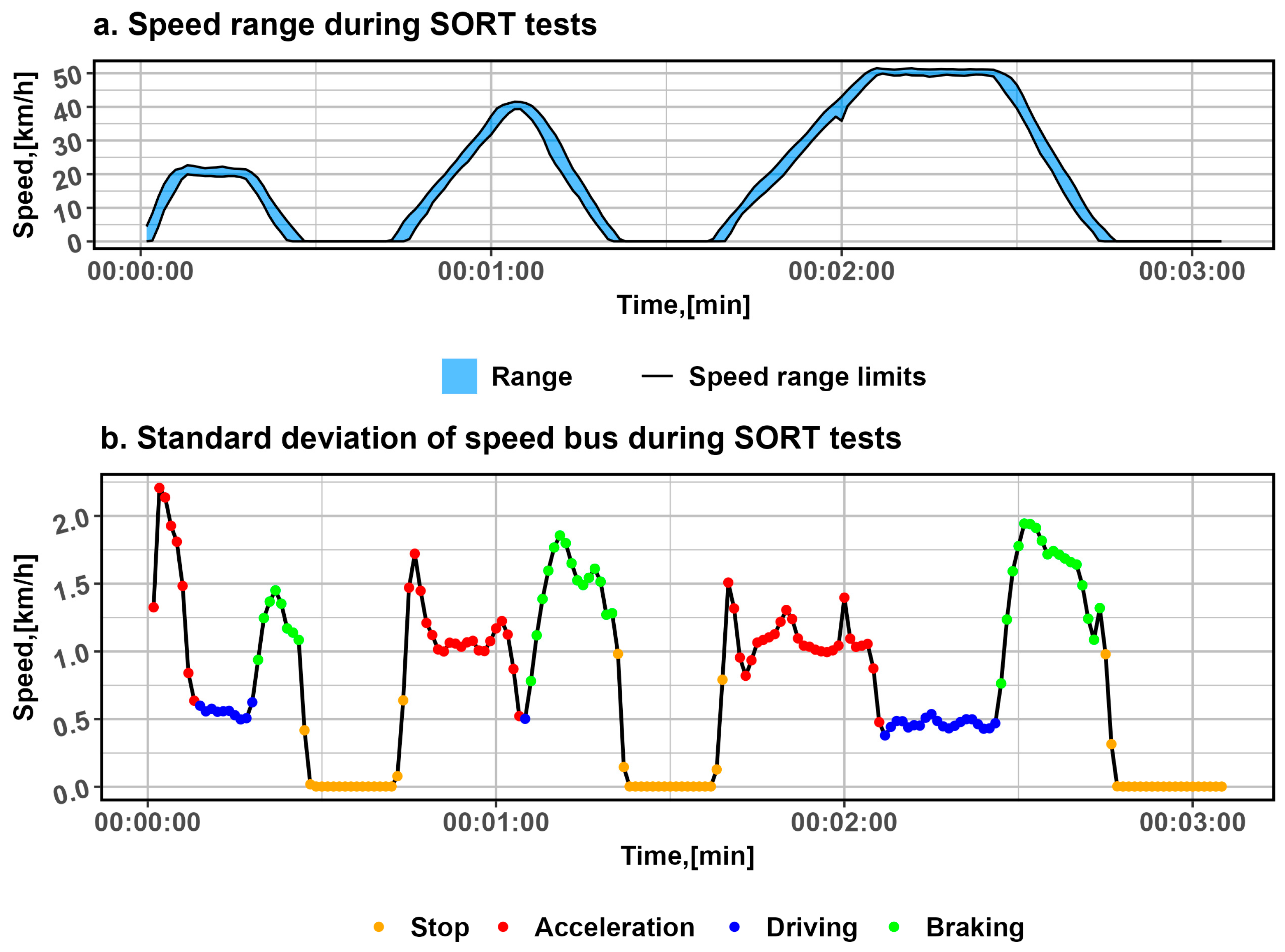Figure 1a shows the area circled in blue, illustrating the range between the highest and lowest speeds at each test moment, while Figure 1b shows the standard deviations as a function of cycle time. To facilitate the analysis of journey repeatability, Figure 1b shows the standard deviation (black curve) of speed measurements during the SORT test, where the states in which the vehicle was moving are marked for each moment.

In the SORT test, the speed pattern reveals recurring intervals of acceleration, uniform-speed operation, deceleration, and halting. The narrow speed range within each phase (Figure 1a) indicates high repeatability, which is crucial for comparing battery types. The standard deviation values (Figure 1b) confirm this stability—the lowest deviations occur during constant speed driving and stopping. In contrast, the highest deviations are observed during acceleration and braking, reflecting the natural speed variability during these phases.

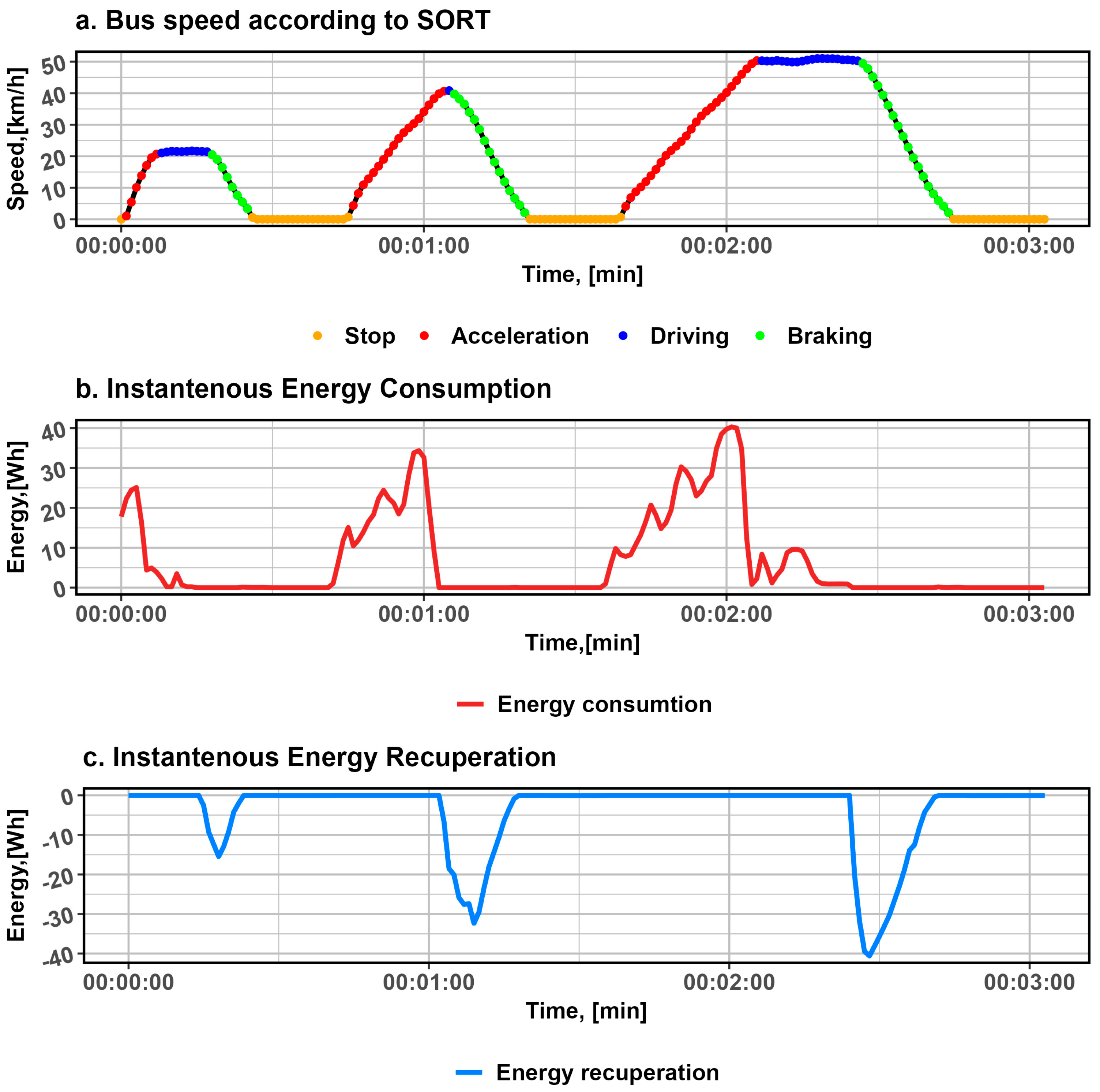
An example SORT test run and electricity consumption for a bus with eight batteries are shown in Figure 2.

The vehicle speed curve (Figure 2a) reflects a typical SORT cycle, with clearly defined standstill phases, acceleration, constant speed, and braking. Instantaneous energy consumption (Figure 2b) peaks during intense acceleration, dropping to almost zero during standstill and coasting. Analysis of instantaneous energy recuperation (Figure 2c) shows significant negative power values during braking, indicating effective energy recovery during these phases. The most significant recuperation potential is observed during the transition from high speed to standstill, which has significant implications for the vehicle’s energy balance.

To evaluate how the number of batteries, acceleration, and speed affect performance, the dataset was split into training (80%) and testing (20%) subsets. The partitioning was performed by vehicle state, with 80% of the records from each state allocated to the training subset and the remaining 20% to the testing subset. This approach decoupled the analysis from the entire trip sequence (time series) and, consequently, from the specific operating conditions of the vehicle.

5.1. Linear Model

Using a linear model (1), we explain the impact of battery capacity, speed, and acceleration on the training set’s IECR. The estimator values, standard deviations of these parameters, the $t_i$ test statistic (11), and $p_i$ the test probability for each parameter are presented in

Table 1. The values of parameters, standard deviation, $t_i$ statistical values, and $p_i$ probability test for the linear model.

	${\mathit{\theta }}_{\mathit{i}}$	${\mathit{S}}_{{\mathit{\theta }}_{\mathit{i}}}$	${\mathit{t}}_{\mathit{i}}$	${\mathit{p}}_{\mathit{i}}$
Intercept	7.7494	0.5992	12.9319	$1.249\times {10}^{-37}$
$v_t$	−0.0199	0.0092	−2.1668	0.0303
$a_t$	−4.8876	0.6160	−7.9340	$2.619\times {10}^{-15}$
$a_t^2$	5.9673	0.5391	11.0685	$3.885\times {10}^{-28}$
$v_t{a}_t$	1.0696	0.0179	59.7217	0
State: braking	−10.8159	0.8578	−12.6087	$6.942\times {10}^{-36}$
State: driving	−4.0014	0.5442	−7.3529	$2.267\times {10}^{-13}$
State: stop	−7.1746	0.6111	−11.7410	$2.097\times {10}^{-31}$
4 batteries	0.1800	0.2568	0.7008	0.4835
8 batteries	0.3663	0.2431	1.5070	0.1319

.

For model (1), the value of the coefficient of determination $R^2$ is 0.7859, which indicates a good fit of the model to the experimental data, with a standard deviation of the residuals of 6.97. Most explanatory variables statistically affect the IECR, including vehicle speed $v_t$, acceleration $a_t$, its square $a_t^2$, and the interaction of speed with acceleration $v_{t}a$. The influence of vehicle operating states, such as braking (braking), driving (driving), and standstill (stop), also turned out to be significant, suggesting that driving dynamics significantly shape IECR.

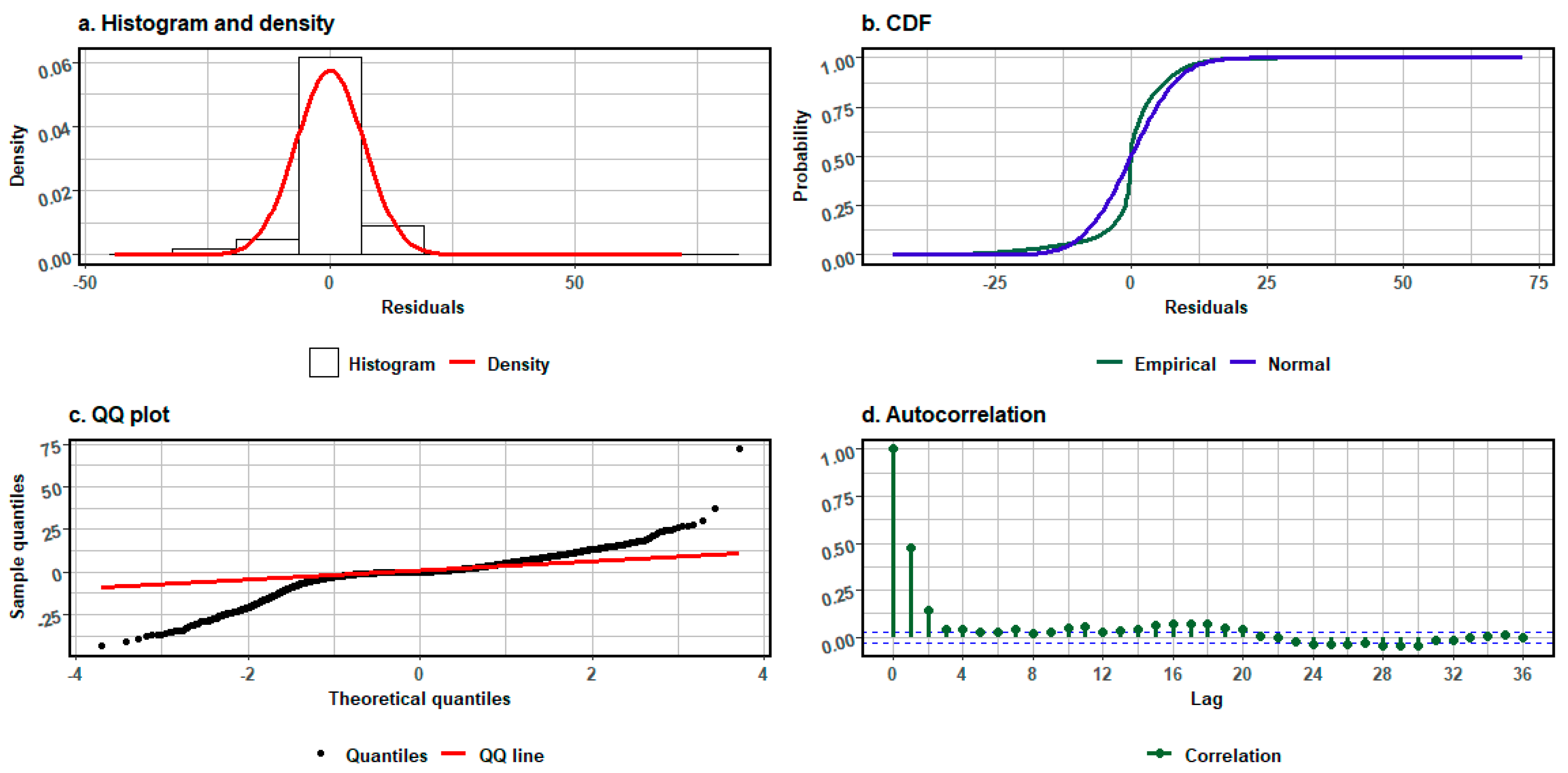
In turn, the number of batteries in the four- and eight-battery configurations is characterised by high test probability values ($p_i>0.05$), indicating a lack of significant effect of this variable on IECR within the adopted linear model. These results suggest that the effect of battery number on energy consumption is only revealed under different operating conditions or is masked by the dominant influence of vehicle motion parameters. For the linear model (1), the residuals were analysed. The graph below shows the histogram, cumulative distribution function, residual autocorrelation, and Q-Q plot (visual verification of the normality postulate of residuals).

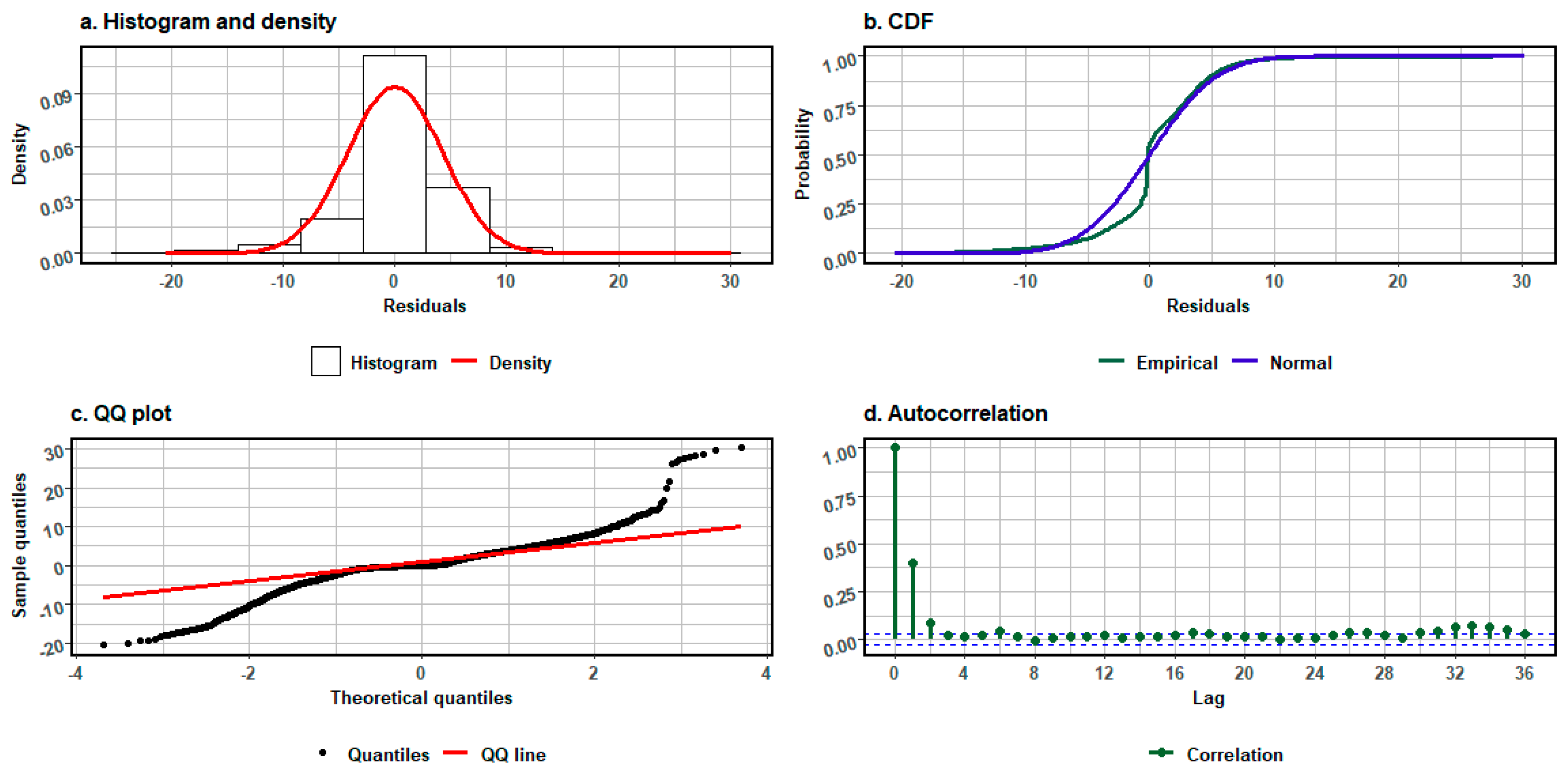
Analysis of the residual series $\{{\epsilon }_t{\}}_{1\le t\le n}$ of the linear model (1), based on Figure 3, indicates the presence of outliers and significant autocorrelation for lags τ = 1 and τ = 2. The distribution of the residuals deviates from normality, as evidenced by the “fat tails” visible in the Q-Q plot and the differences between the empirical and theoretical distribution functions. The histogram and density function reveal asymmetry and a greater concentration of values around zero, but with a few outlying observations. These results suggest that the assumptions regarding normality and independence of the residuals are not fully met, which may indicate the influence of additional factors not accounted for in the model.

We used the Shapiro–Wilk, Cramér–von Mises, Anderson–Darling, Lilliefors (Kolmogorov–Smirnov), D’Agostino Omnibus, and Jarque–Bera tests, as well as the independence of the residuals using the Ljung-Box test for shifts $1\le \tau \le 10$.

Table 2. Results of normality and residual correlation tests for the linear model.

Test	Statistics	p-Value
Shapiro–Wilk normality test	0.8330	0
Anderson–Darling test	260.7239	0
Cramér–von Mises test	51.7989	0
Lilliefors (Kolmogorov–Smirnov) test	0.1912	0
Jarque–Bera test	14,838.5399	0
D’Agostino Omnibus test	1496.8640	0
Ljung–Box test	1233.4281	0

provides the statistics and test probability values.

Analysis of the distribution of the linear model residuals revealed significant deviations from normality. All tests performed, Shapiro–Wilk, Cramér–von Mises, Anderson–Darling, Lilliefors (Kolmogorov–Smirnov), D’Agostino Omnibus, Jarque–Bera, and Ljung–Box, yielded test probability values close to zero, which is below the significance level of α = 0.05, so the hypotheses of a normal distribution of residuals should be rejected.

Such consistent results across all tests suggest that the residuals exhibit substantial deviations from normality, which may result from non-linear relationships between variables, the presence of outliers, or heteroscedasticity. The results of the Ljung–Box test additionally indicate the presence of autocorrelation in the residuals, which may indicate the validity of considering models with a different structure, e.g., non-linear or recurrent neural networks.

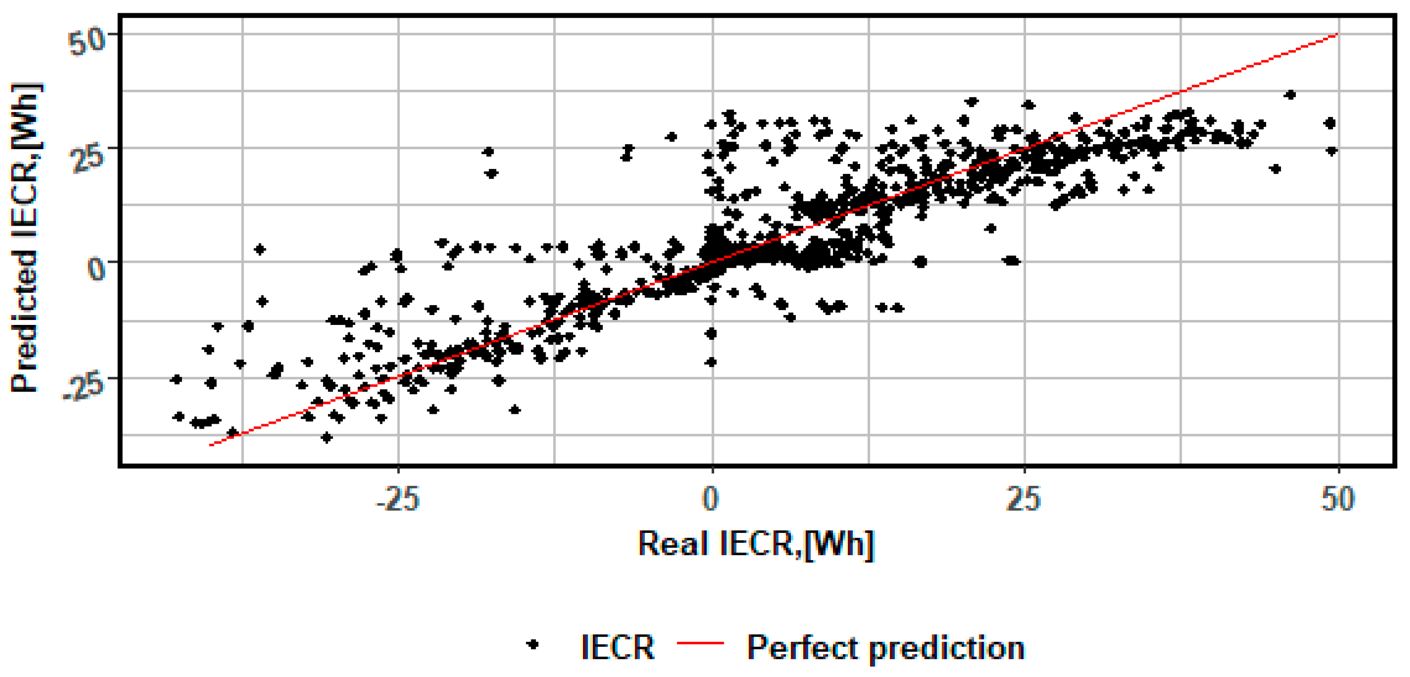
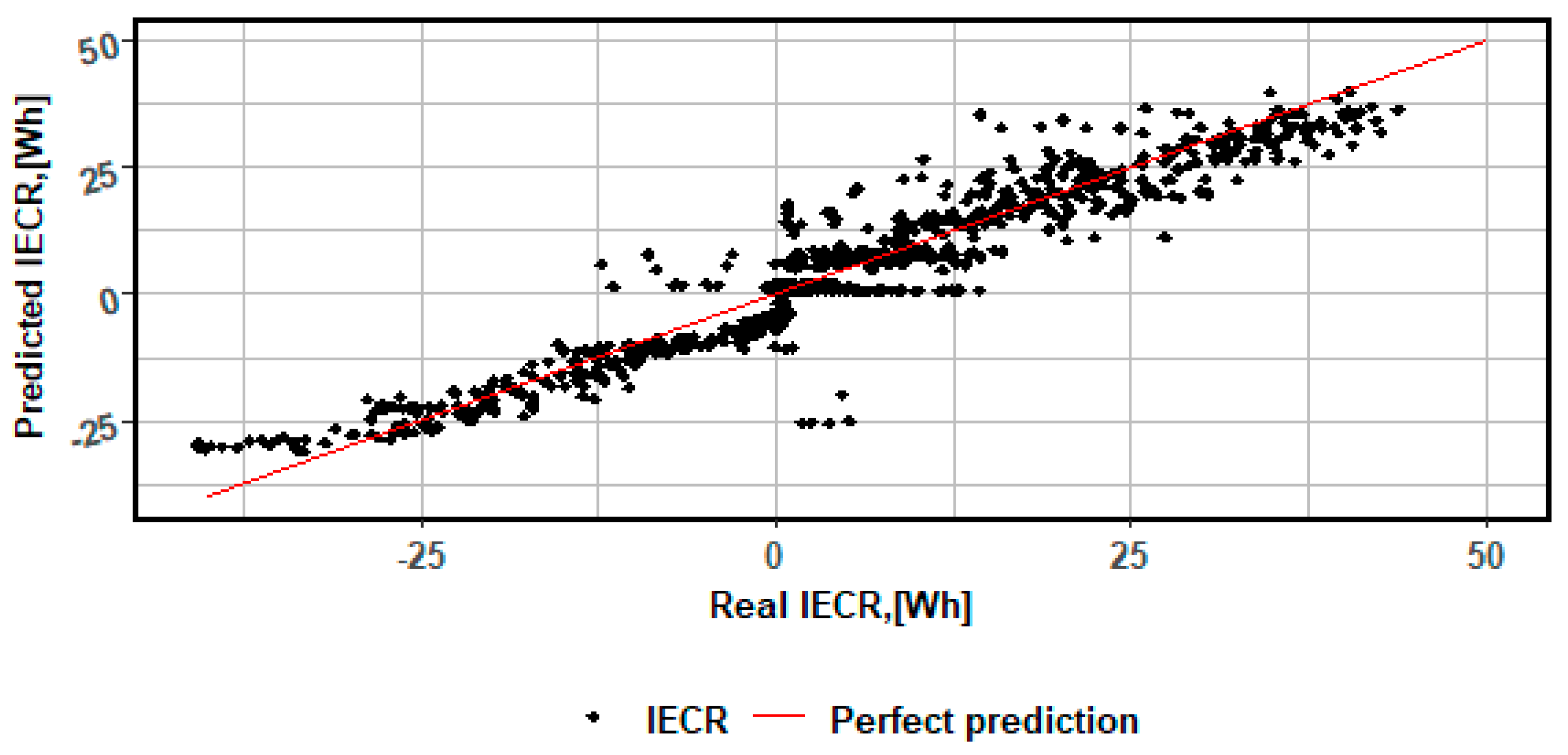
Then, model (1) was validated on the test set. Figure 4 shows the actual and predicted values of the IECR.

A comparison of actual and predicted values for instantaneous energy consumption and recovery indicates a good agreement with the linear model concerning the overall trend. Data points are distributed along the red line (the line of perfect agreement between actual and predicted values). However, some scatter is visible, particularly for extreme positive and negative values. This scatter suggests that the model may have limited accuracy in predicting extreme energy consumption and recovery values, which may be due to non-linear relationships not captured by the model. Nevertheless, prediction accuracy is relatively high within the range of average values.

5.2. Extended Linear Model Concerning States

For model (4) for the acceleration state, the values of the estimators, standard deviations of these parameters, the value of $t_i$ the test statistic (11), and $p_i$ the test probability for each parameter are presented in

Table 3. The values of parameters, standard deviation,${ t}_i$ statistical values, and $p_i$ probability test for the linear model for the acceleration state.

	${\mathit{\theta }}_{\mathit{i}}^{\mathit{A}}$	${\mathit{S}}_{{\mathit{\theta }}_{\mathit{i}}}$	${\mathit{t}}_{\mathit{i}}$	${\mathit{p}}_{\mathit{i}}$
Intercept	4.7581	0.6251	240.6906	0
4 batteries	1.2854	0.4177	97.3119	0
8 batteries	3.3831	0.4325	247.3615	0
$v_t$	0.0069	0.0175	12.4784	8.999 × 10−36
$a_t$	0.5345	0.7113	23.7639	8.862 × 10−122
$a_t^2$	0.0120	0.0995	3.8072	7.069 × 10−5
$v_t{a}_t$	1.2276	0.0446	870.7524	0

.

In the case of the linear model describing the acceleration condition, all main variables showed a significant effect on the explained variable, at a significance level of α = 0.05. The parameters of the number of batteries (both four- and eight-battery configurations) are statistically significant, indicating a noticeable effect of the power supply configuration on the IECR value during acceleration. The speed variable $v_t$, acceleration $a_t$, and their interactions $v_t{a}_t$ are characterised by very high statistical values $t_i$ and $p_i$, values close to zero, confirming their key role in the model. The value for the component $a_t^2$ is also significant, although with a higher p-value compared to the other predictors. Such a high level of significance for parameters related to driving dynamics suggests that in the acceleration state, the variability of the IECR is strongly dependent on vehicle speed and acceleration, and the effect of battery number, although smaller than that of the motion parameters, remains significant.

For model (4) for the braking state, the values of the estimators, the standard deviations of these parameters, the value $t_i$ test statistic (11), and $p_i$ the test probability for each parameter are presented in

Table 4. The values of parameters, standard deviation, statistical $T$ values, and test probability for the linear model for the braking state.

	${\mathit{\theta }}_{\mathit{i}}^{\mathit{B}}$	${\mathit{S}}_{{\mathit{\theta }}_{\mathit{i}}}$	${\mathit{t}}_{\mathit{i}}$	${\mathit{p}}_{\mathit{i}}$
Intercept	−1 × 10−9	6.1195 × 10−16	−51,675,295.49	0
4 batteries	−1.27 × 10−9	4.3039 × 10−17	−734,749,089.34	0
8 batteries	−0.4778	0.2974	−50.8013	0
$v_t$	−0.4649	0.0219	−672.3865	0
$a_t$	5.103 × 10−19	1.942 × 10−15	0.0083	0.4967
$a_t^2$	−1.726 × 10−17	9.126 × 10−16	−0.5982	0.2749
$v_t{a}_t$	0.2785	0.0303	290.3297	0

.

For the linear model describing the braking state, most of the parameters were highly statistically significant, and the $p_i$ test probability values were close to zero, which indicates their strong influence on IECR in this driving phase. The configuration of the number of batteries (four- and eight-battery configurations), the variable speed, and the product of velocity and acceleration are significant at a level bordering on absolute statistical certainty.

The structural parameters with acceleration variables $a_t$ and the square of acceleration $a_t^2$ show higher $p_i$ test probability values, which suggests a minor role of these variables in the energy recovery process during braking compared to $v_t$ the vehicle speed and the interaction $v_t{a}_t$ of speed and acceleration. The interactive component, in turn, $v_t{a}_t$ is significant and reflects the intricate interplay of speed and acceleration during energy recuperation.

The results indicate that in the braking state, the dominant factor determining the IECR is the vehicle speed, the product of acceleration and speed, and the number of batteries. In contrast, the influence of acceleration is complementary.

For model (4) for the driving state, the values of the estimators, standard deviations of these parameters, the value $t_i$ test statistic (11), and $p_i$ the test probability for each parameter are shown in

Table 5. The values of parameters, standard deviation $t_i$ statistical values, and $p_i$ probability test for the linear model for the driving state.

	${\mathit{\theta }}_{\mathit{i}}^{\mathit{D}}$	${\mathit{S}}_{{\mathit{\theta }}_{\mathit{i}}}$	${\mathit{t}}_{\mathit{i}}$	${\mathit{p}}_{\mathit{i}}$
Intercept	−1.7340	0.4654	−3.7260	0.0002
4 batteries	0.2915	0.3148	0.9261	0.3548
8 batteries	0.2049	0.2977	0.6881	0.4917
$v_t$	0.1751	0.0094	18.6364	3.998 × 10−62
$a_t$	−13.0527	9.3604	−1.3944	0.1637
$a_t^2$	−73.5850	57.7703	−1.2738	0.2032
$v_t{a}_t$	0.7112	0.2179	3.2633	0.0012

.

Due to the linear model describing the driving state (driving), the analysis indicates that, of all variables, only speed $v_t$ and the interactive term $v_t{a}_t$ significantly affect IECR ($p_i$< 0.05). The test probability value for speed is extremely low, $3.998\times {10}^{-62}$, which confirms its dominant influence on IECR in the steady-state driving phase.

In turn, the number of batteries (both four- and eight-battery configurations) and acceleration-related variables ($a_t i a_t^2)$ do not reach statistical significance, suggesting that they have limited significance in this condition. The intercept in the model is also significantly different from zero.

For model (4) for the stop state, the values of the estimators, the standard deviations of these parameters, the value $t_i$ test statistic (11), and $p_i$ the test probability for each parameter are presented in

Table 6. The values of parameters, standard deviation, statistical $T$ values, and test probability for the linear model for the stopped state.

	${\mathit{\theta }}_{\mathit{i}}^{\mathit{S}}$	${\mathit{S}}_{{\mathit{\theta }}_{\mathit{i}}}$	${\mathit{t}}_{\mathit{i}}$	${\mathit{p}}_{\mathit{i}}$
Intercept	0.7690	0.0436	17.6492	5.463 × 10−63
4 batteries	0.0102	0.0614	0.1660	0.8682
8 batteries	−0.0734	0.0611	−1.202	0.2296

.

In the model describing the stopped state (stop), the only statistically significant parameter is the intercept (intercept), whose value is positive (${\theta }_0^D=0$.769), and the test probability is 5.463 × 10⁻⁶³ (below the significance level of 0.05), which indicates that the average energy consumption is 0.769 Wh during the stopped state. Neither the number of batteries in the four- nor eight-battery configuration significantly affects the dependent variable IECR (for these structural parameters, the test probability is above the significance level of 0.05).

Model (4) is characterised by a high value of the coefficient of determination $R^2$= 0.9124, which means that it reasonably reflects the variability of IECR in the states of acceleration, braking, driving, and stopping, with a low standard deviation of the residuals equal to 4.2648.

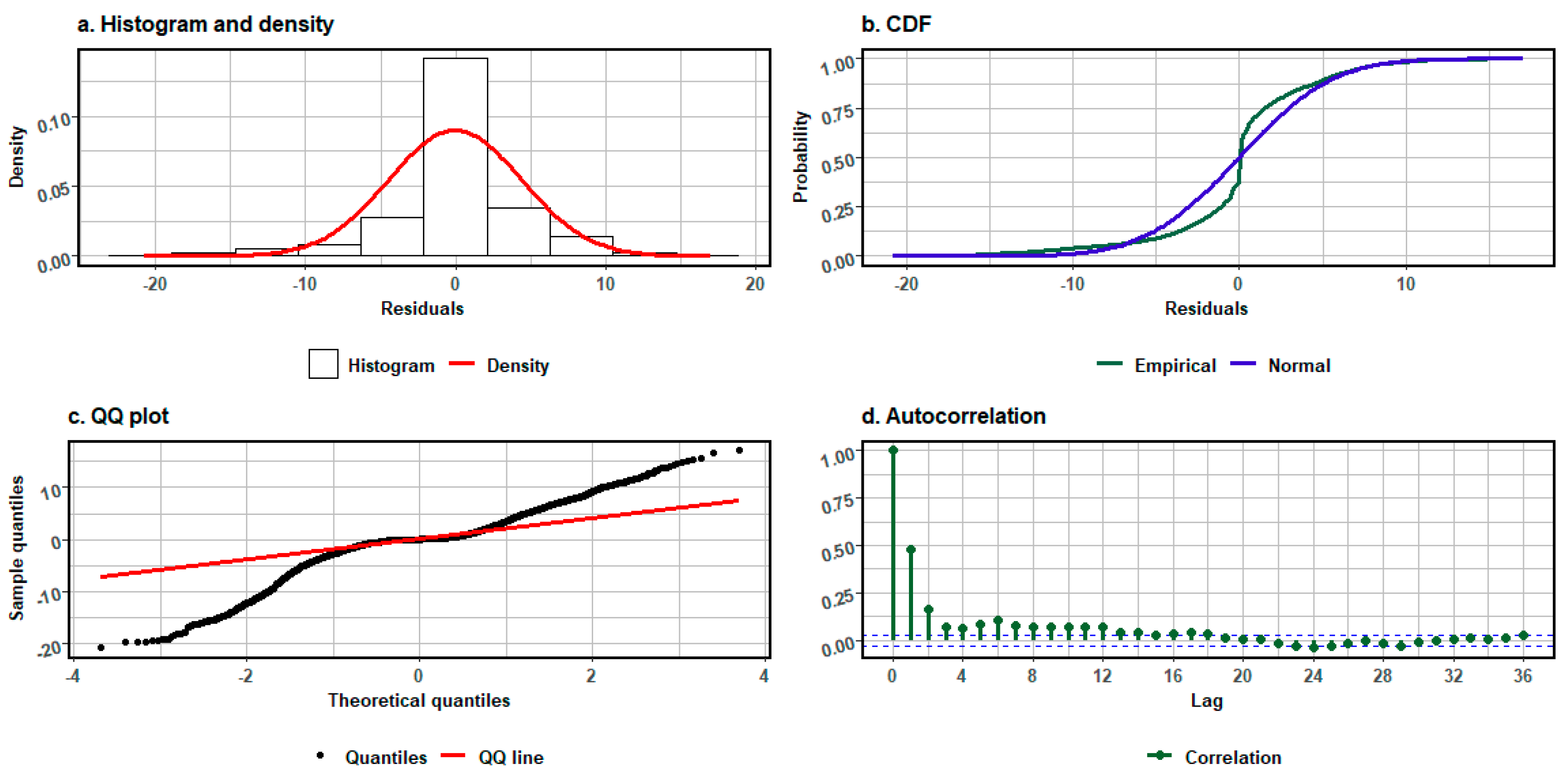
For the ELM (4), the residuals were analysed. Figure 5 presents the histogram, cumulative distribution function, autocorrelation of the residuals, and Q-Q plot.

The analysis of the residuals for model (4) indicates the presence of extreme values in the series $\{{\epsilon }_t{\}}_{1\le t\le n}$ and a significant autocorrelation for the τ shifts ∈ {1, 2}. The histogram and density function reveal a distribution close to normal, although with visible “fat tails”, as confirmed by the Q-Q plot. The empirical distribution function differs from the theoretical normal distribution function, but the agreement is better than the baseline model (1). Statistical tests (Shapiro–Wilk, Cramér–von Mises, Anderson–Darling, Jarque–Bera, Lilliefors/Kolmogorov–Smirnov, D’Agostino Omnibus) confirm deviations from normality, and the Ljung–Box test for shifts 1 ≤ τ ≤ 10 indicates partial dependence between subsequent residuals. The values of the statistics and test probabilities are summarised in

Table 7. Results of normality tests and correlation tests for residuals of the linear model with states.

Test	Statistics	p-Value
Shapiro–Wilk normality test	0.8996	0
Anderson–Darling test	131.9078	0
Cramér–von Mises test	26.4533	0
Lilliefors (Kolmogorov–Smirnov) test	0.1580	0
Jarque–Bera test	7067.8145	0
D’Agostino Omnibus test	651.1530	0
Ljung–Box test	769.2797	0

.

On normality tests (Shapiro–Wilk, Anderson–Darling, Cramér–von Mises, Lilliefors, Jarque–Bera, D’Agostino Omnibus), we see very low test probability values (below the 0.05 significance level), which indicates the rejection of the hypothesis of normality of the residual distribution in the model considering job states. Additionally, the Ljung–Box test confirms the presence of autocorrelation in the residuals. This indicates that model (4) fits the data better than model (1); however, the distribution of the residuals deviates from normality and shows significant time dependence.

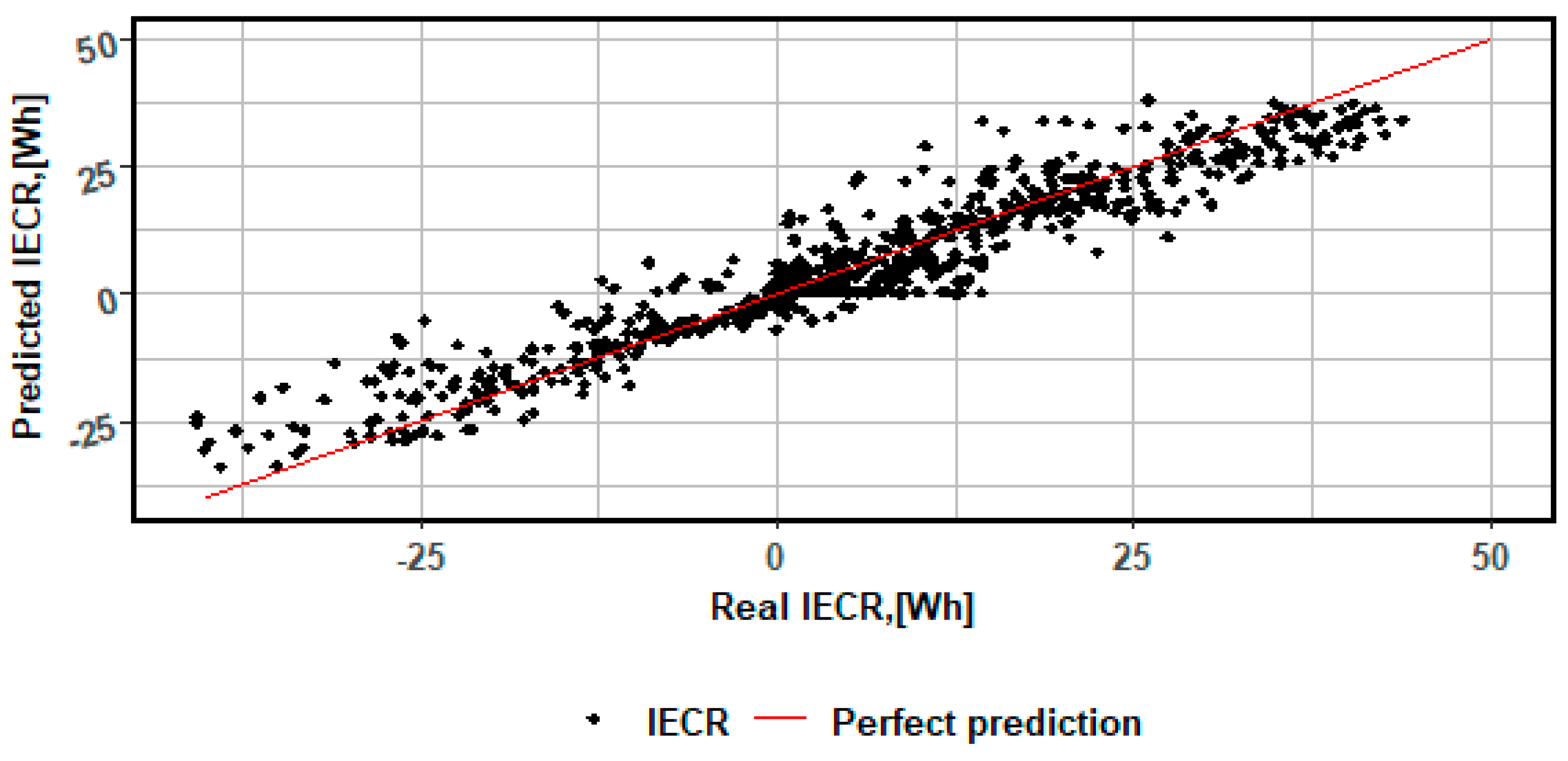
Then, model (4) was validated on the test set. Figure 6 shows the actual and predicted values of the instantaneous energy consumption and recuperation.

The model validation (4) results on the test set demonstrate good agreement between the actual and predicted values of IECR. The points align along the perfect fit line (red line), confirming high prediction accuracy. However, a greater discrepancy is visible at the extreme values, possibly due to the smaller number of observations in these ranges and non-linear effects not captured by the linear model.

5.3. Neural Network

For the neural network without regularisation (${\lambda }_1=0$, ${\lambda }_2=0$) and with the dropout technique applied (20%), the dependency model is presented in

Table 8. NN architecture without regularisation (dropout 20%).

Layer (Type)	Output Shape	Parameters	Activation
Input Layer	(None, 11)
Dense 1	(None, 10)	120	Linear
Dropout	(None, 10)	0
Dense 1	(None, 5)	55	Linear
Output Dense	(None, 1)	6	Linear

.

The neural network model consists of five layers: an input layer with 11 features, two dense layers with ten and five neurons, respectively, a dropout layer to reduce the risk of overfitting, and an output layer with a single neuron. All dense layers use a linear activation function, which is justified by the nature of the regression problem. The total number of parameters is 181.

On the training set, the coefficient of determination $R^2$ for the NN is 0.9059, while the standard deviation of the residuals is 4.4332. The residuals were analysed for the neural network, and the visual analysis is presented in Figure 7.

The figure shows the occurrence of extreme values in a series of residuals $\{{\epsilon }_t{\}}_{1\le t\le n}$ and a significant correlation with lag $\tau \in \{1,\dots ,12\}$. The Q-Q plot reveals “fat tails”, and comparing the empirical and theoretical (normal) distribution functions indicates significant deviations from the normal distribution. The normality of the residual distribution was verified using the Shapiro–Wilk, Anderson–Darling, Cramér–von Mises, Lilliefors (KS), Jarque–Bera, and D’Agostino Omnibus tests, and independence was verified using the Ljung–Box test for 1 ≤ τ ≤ 10. Detailed results are presented in

Table 9. Results of normality tests and correlation tests for residuals of the neural network.

Test	Statistics	p-Value
Shapiro–Wilk normality test	0.9008	0
Anderson–Darling test	179.6719	0
Cramér–von Mises test	37.1023	0
Lilliefors (Kolmogorov–Smirnov) test	0.1578	0
Jarque–Bera test	2255.0859	0
D’Agostino Omnibus test	689.9610	0
Ljung–Box test	1372.5825	0

.

Table 9 presents the results of eight statistical tests (normality and autocorrelation) for the neural network model residuals. For each test, the test probability value is significantly below the 0.05 significance level, indicating rejection of the null hypothesis of normality in the residuals. The results of the Jarque–Bera, D’Agostino Omnibus, and Ljung–Box tests confirm that the residuals exhibit both significant deviations from normality and autocorrelation. The neural network model presented in Table 8, as well as models (1) and (4), do not fully reflect the data’s variability structure.

Figure 8 compares actual and predicted values for IECR obtained from the NN model. A strong correlation is visible between the observed data and the predictions, with most points falling along the red line (the line of perfect fit), confirming the model’s high agreement with reality. Deviations from the red line mainly concern extreme values, where greater scatter in the predictions appears.

5.4. Recurrent Neural Network

For the recurrent neural network without regularisation and with the dropout technique (20%), the dependency model is presented in

Table 10. RNN architecture without regularisation (dropout 20%).

Layer (Type)	Output Shape	Parameters	Activation
Input Layer	(None, 11)	0
Dense 1 (Simple RNN)	(None, 11, 8)	80	Linear
Dropout	(None, 11.8)	0
Dense 2 (Flatten)	(1, 88)	0	$-$
Dense 2	(1, 5)	445	Linear
Output Dense	(1, 1)	6	Linear

.

Table 10 shows the detailed architecture of the recurrent neural network without regularisation, which uses a 20% dropout technique. The table shows the type and order of layers, the shape of the output data, the number of trainable parameters, and the activation functions used in each layer. The total number of model parameters is 531, including weights and biases of all layers.

On the training set, the coefficient of determination $R^2$ for the RNN is 0.9343, while the standard deviation of the residuals is 3.7047. The residuals were also analysed for the neural network. Figure 9 presents the histogram, cumulative distribution function, Q-Q plot, and autocorrelation of the residuals.

The residuals reveal the presence of extreme values in the residual series $\{{\epsilon }_t{\}}_{1\le t\le \mathrm{n}}$ and significant autocorrelation for the shifts τ ∈ {1, 2, 5… 12}. The Q–Q plot indicates the presence of “fat tails”, and comparing cumulative distribution functions confirms apparent differences between the theoretical and empirical normal distributions. The normality of the residual distribution was verified using the Shapiro–Wilk, Cramér–von Mises, Anderson–Darling, Lilliefors (Kolmogorov–Smirnov), Jarque–Bera, and D’Agostino Omnibus tests, while the independence of the residuals was checked using the Ljung–Box test for shifts 1 ≤ τ ≤ 10. The results of the statistics and test probabilities are shown in

Table 11. Results of normality tests and correlation tests for residuals of the recurrent neural network.

Test	Statistics	p-Value
Shapiro–Wilk normality test	0.8769	0
Anderson–Darling test	180.4883	0
Cramér–von Mises test	37.5676	0
Lilliefors (Kolmogorov–Smirnov) test	0.1650	0
Jarque–Bera test	8241.3118	0
D’Agostino Omnibus test	1154.2360	0
Ljung–Box test	750.2810	0

.

Table 11 shows the results of normality tests and correlation tests for the residuals of the RNN for the Shapiro–Wilk, Cramér–von Mises, Anderson–Darling, Lilliefors (Kolmogorov–Smirnov), Jarque–Bera, D’Agostino Omnibus, and Ljung–Box tests. All test probability values are below the 0.05 significance level, indicating a significant deviation of the residual distribution from normality and correlation in the time series.

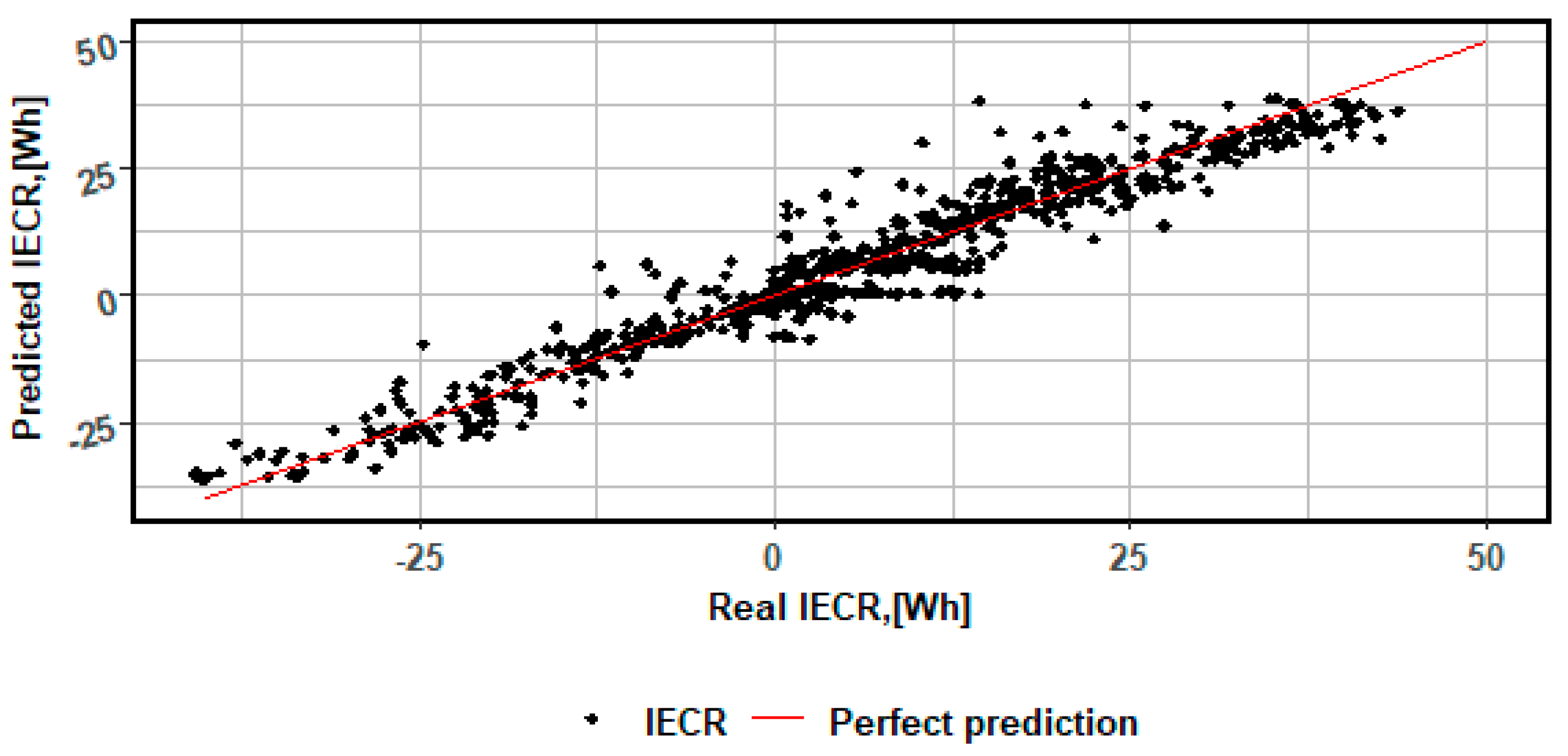
Figure 10 compares actual and predicted instantaneous energy consumption values obtained from the RNN. The distribution of points along the perfect fit line indicates a high degree of agreement between the predictions and the measurements. However, a greater scatter is visible for the extreme values, particularly in high and low energy consumption areas.

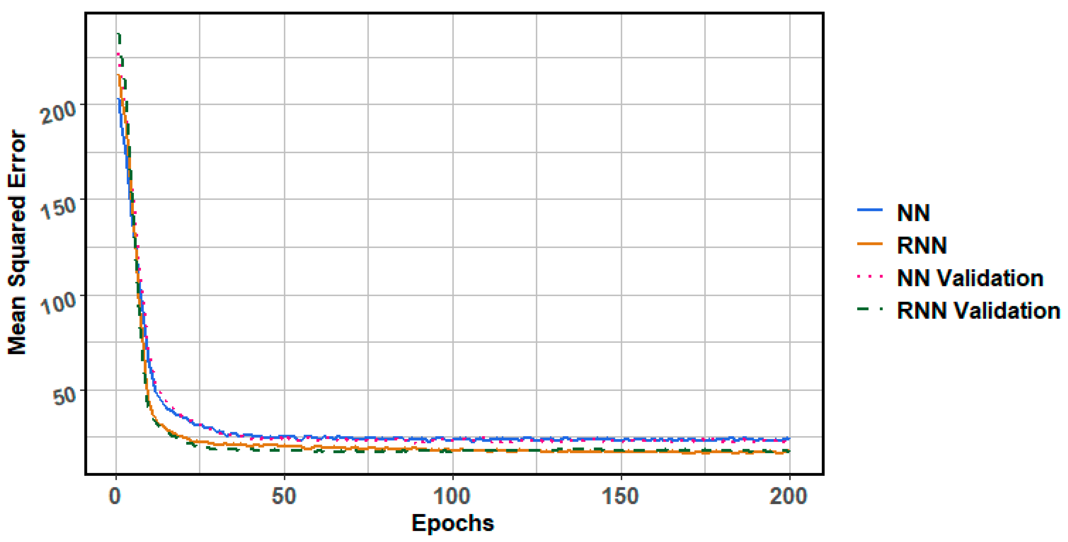
Figure 11 shows the speed and quality of learning for the neural network models. The batch was divided into two parts for each epoch: 85% was used for training the network and 15% was used for validation. The training process involved 200 epochs.

Figure 11 shows the training curves of a classical NN and RNN, along with their corresponding validation curves. Both models exhibit a sharp decline in the Mean Squared Error in the initial epochs, followed by a stabilisation at a low level after approximately 50 epochs. This curve indicates an effective model fit and no signs of overfitting.

5.5. Prediction Comparison

To compare the predictions of the models on the test set, the correlation coefficient ($r$) between the actual and predicted values was estimated. Instantaneous energy consumption and recuperation, Mean Squared Error (MSE), Root Mean Squared Error (RMSE), and Mean Absolute Error (MAE) were evaluated. The values these coefficients (16)–(19) represent are shown in

Table 12. The correlation coefficient, Mean Squared Error, Root Mean Squared Error, and Mean Absolute Error for models on the test set.

	r	MSE	RMSE	MAE
Linear Model	0.8864878	48.49007	6.963481	4.047660
Extended Linear Model	0.9557132	18.18811	4.264752	2.747482
Neural Network	0.9531719	19.65345	4.433222	2.755827
Recurrent Neural Network	0.9666154	13.72478	3.704697	2.241747

.

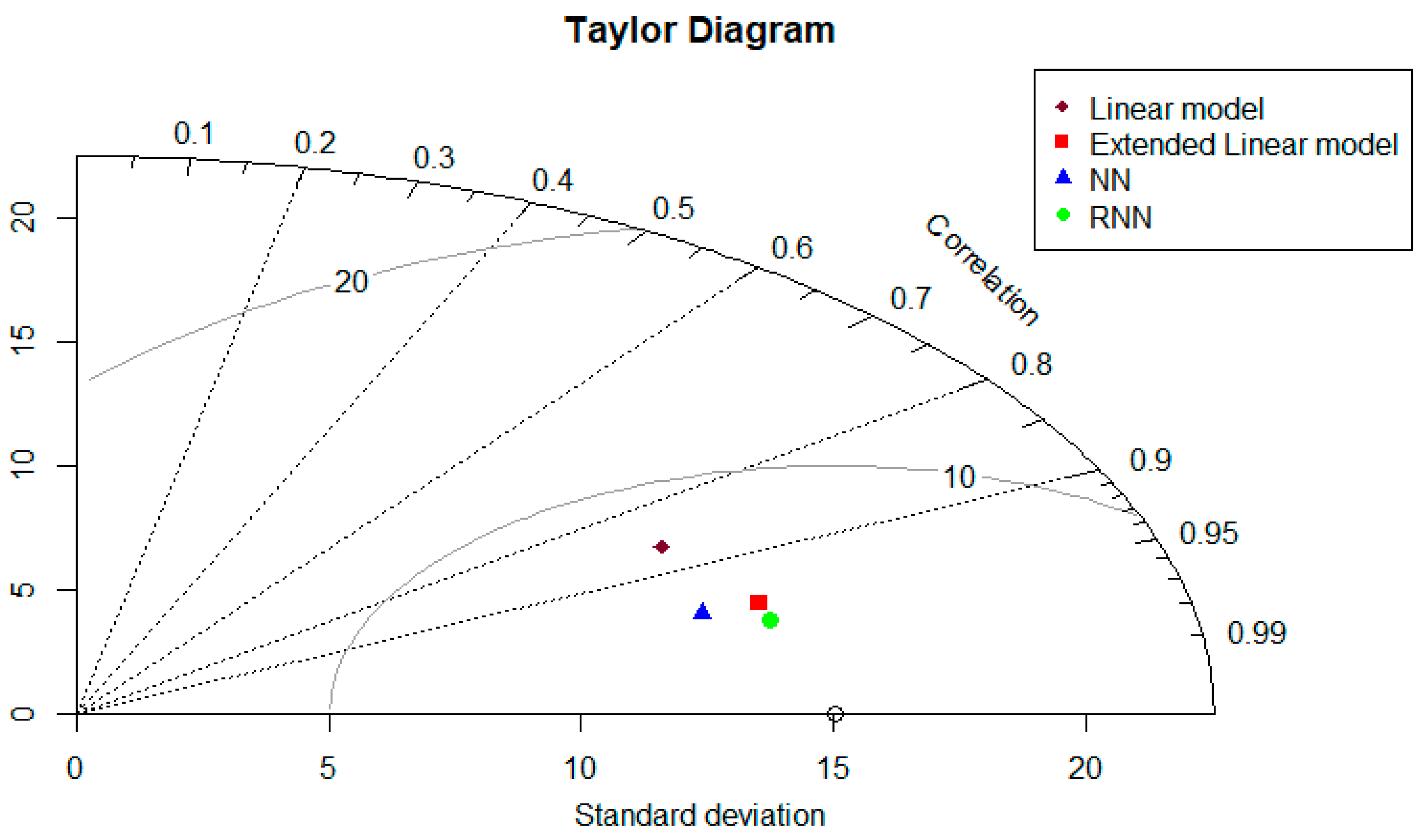
Table 12 compares the prediction quality of four models: linear, extended linear, neural network, and recurrent neural network. The best prediction results were obtained for the recurrent neural network, characterised by the highest correlation coefficient (r = 0.9666) and the lowest error values (MSE = 13.72; RMSE = 3.70; MAE = 2.24), indicating its highest accuracy in representing the test data. The Taylor diagram illustrates the graphical agreement between the models and the reference data.

The Taylor diagram (Figure 12) illustrates the fit of four models: linear model, extended linear model, classical neural network, and recurrent neural network (RNN). Both neural models have the highest correlation coefficient (above 0.95) and a standard deviation close to the reference value, indicating greater precision in representing the data than linear models.

6. Discussion of the Results

During SORT tests, the analysis of IECR in electric buses revealed a clear impact of both driving parameters (speed, acceleration) and battery configuration on vehicle energy efficiency. The obtained results confirm observations from the literature that driving profile—particularly acceleration intensity and frequency—is a key factor determining instantaneous energy consumption [40,41].

A comparison of three vehicle configurations (one battery with a pantograph, four batteries, eight batteries) showed that increasing the number of batteries. Therefore, vehicle weight leads to a noticeable increase in energy consumption during acceleration. This effect is consistent with previous studies, which indicate a significant role of the total vehicle weight in shaping energy losses, especially on routes with frequent speed changes [42,43]. At the same time, larger battery capacity promotes range extension, but, as emphasised by Yin et al. [48], this increase becomes increasingly inefficient above a certain threshold, and excessive weight increases can negatively impact the overall energy balance.

Regarding energy recovery, the obtained results confirm that its effectiveness is closely related to braking dynamics. Intensive braking phases generated higher energy recovery, which is consistent with the results of studies that strategies based on higher braking force values allow for the recovery of 25–51% of kinetic energy [15,48]. For the cases examined, the ratio of recovered to consumed energy corresponded to values reported in the literature. Nevertheless, refinements to the braking strategy, such as the application of fuzzy control or threshold algorithms, may further raise this indicator and improve the efficiency of the system as a whole [63].

The applied modelling approaches confirmed that non-linear models (NNs and RNNs) better represent the complex relationships between IECR and driving parameters than linear models. Higher values of the coefficient of determination and lower prediction errors (RMSE, MAE) for neural networks indicate their greater ability to capture non-linearities characteristic of real-world driving profiles. These results are consistent with the observations of other authors, according to which recurrent architectures (LSTM, GRU) provide perfect accuracy in the analysis of temporal data in transport [37,38]. The extended linear model, concerning vehicle states, illustrates the dependencies between the vehicle driving dynamics, the number of batteries installed in the bus, and NN models.

Analysis of the impact of driving states revealed that the most significant differences between linear and non-linear models occurred during acceleration phases, where power demand is highest. These differences were less significant during constant speed and standstill phases, confirming that the main benefits of advanced modelling are related to conditions of high-speed variability. These results fit into the broader literature context, which indicates the need for adaptive, scenario-specific predictive models in public transport [4].

The strict implementation of the speed profile consistent with the SORT methodology ensured the high repeatability of the measurement results, which enables direct comparisons between the tested variants. SORT, as a method for assessing the energy efficiency of entire vehicles in near-real-world conditions, remains an indispensable tool in research on public transport optimisation [4,5].

Based on the present findings, the most critical next step for validating and deploying the proposed modelling approach is systematically collecting and integrating real-world operational data. While SORT tests ensure high repeatability and provide reliable benchmarks, they cannot fully capture the stochastic variability of urban traffic, driver behaviour, and environmental conditions. Extending the models with operational datasets would allow for assessing their robustness in diverse scenarios and strengthening their applicability to fleet-level decision-making, including scheduling and charging optimisation. Testing under different climatic conditions and accounting for operational factors such as breakdowns, defects, or battery degradation remain important complementary directions; however, immediate priority should be given to verifying model fidelity against in-service data.

In summary, the obtained results confirm the following:

• The number of batteries significantly influences the instantaneous energy consumption, especially during dynamic driving phases.
• The effectiveness of recuperation depends on the braking strategy and can be increased by implementing advanced control methods.
• The extended linear model concerning states is more straightforward to interpret and simple to adapt for IECR prediction; on the other hand, the quality of prediction is comparable to neural networks.
• Neural network models are more effective than classical linear models in predicting IECR, especially under conditions of high-speed variability.
• Standardisation of test conditions (SORT) is crucial for reliable comparison of configurations and energy efficiency evaluation.

7. Conclusions

The analysis was conducted to compare the effectiveness of linear models and neural networks, including recurrent architectures, in predicting instantaneous energy consumption and recuperation. The linear models, both the baseline (1) and the extended model with state variables (4), achieved coefficients of determination of 0.7859 and 0.9124, respectively, in the extended version. However, parameter analysis revealed that not all explanatory variables were statistically significant for the classic model—for example, the number of batteries, whose effect on IECR was insignificant. It is worth emphasising that the extended linear model showed that vehicle dynamics and battery number may be crucial for estimating the IECR prediction for different states. Analysis of the residuals revealed the presence of outliers, significant time correlations in the range τ ∈ {1,…,12}, and apparent deviations from the normality of the distribution, as confirmed by the Shapiro–Wilk, Anderson–Darling, Lilliefors, Cramér–von Mises, Jarque–Bera, and D’Agostino Omnibus tests, while the Ljung–Box test additionally indicated the lack of independence of the residuals.

Using a classical neural network allowed for a significantly higher coefficient of determination $R^2$ (around 0.91) with a lower standard deviation of the residuals. The values of $R^2$ for the extended linear model concerning states and the neural network models are very similar. Fit plots confirmed excellent agreement of the forecasted values with the actual data, especially in the range of average loads. However, analysis of the residuals still revealed the presence of extreme values and “fat tails” of the distribution and temporal correlations for selected delays. Introducing a recurrent architecture (RNN) further improved the accuracy of short-term forecasts, especially during rapid load changes and transitions between energy consumption and recuperation phases. Fit plots for the RNN were characterised by minimal phase shifts relative to the actual data, indicating a good ability to represent the dynamics of the processes. However, “fat tails” and some temporal correlations were still observed in the residuals for selected delays.

A comparison of the model fit and stability based on the Taylor diagram and summary indices demonstrated the advantage of neural models over linear models. NN models, particularly RNNs, achieved better correlation with measured data, lower RMSD errors, and minor shifts in the amplitude of IECR changes. The neural network training process was stable over 200 epochs, with the data divided into training (85%) and validation (15%), which avoided overfitting. The results indicate that the most effective approach for applications requiring high-precision representation of instantaneous IECR values is to use neural architectures, especially recurrent ones, due to their ability to model temporal dependencies. Linear models are more easily interpretable and can be used in simplified cases requiring low computational complexity; however, their limited flexibility translates into larger fitting errors. However, concerning states, the extended linear model achieved prediction accuracy comparable to that of neural networks. Regardless of the method used, it may be important to implement techniques that limit the influence of outliers and eliminate temporal correlations in the residuals. At the same time, further research may include expanding the set of variables with additional parameters describing the vehicle state and environmental conditions, as well as testing hybrid architectures combining RNNs with attention mechanisms.