Abstract
In closed Brayton cycle power generation systems, sudden load disturbances can induce a compressor surge in turbine–alternator–compressor systems, posing significant risks to dynamic stability and operational reliability. To address this challenge, this study proposes a PID control strategy optimized via a genetic algorithm. A high-fidelity dynamic model of the turbine–alternator–compressor system under closed Brayton cycle conditions is developed in Simulink, incorporating surge boundaries derived from performance maps. Control parameters are tuned using a weighted multi-objective fitness function that integrates overshoot, rise time, and the integral of absolute error. Simulation results demonstrate that the proposed control scheme markedly enhances system responsiveness—achieving approximately a 70% improvement in rotational speed regulation—and effectively maintains the operating point outside the surge region. The proposed framework provides a practical and robust approach for improving the dynamic stability and reliability of closed Brayton cycle power generation systems.
1. Introduction
The increasing demands for high power density, operational reliability, and efficient thermal management in modern energy systems have revealed the limitations of conventional technologies, such as chemical propulsion and thermoelectric conversion [1,2,3]. As a promising alternative, the closed Brayton cycle (CBC) has attracted significant attention due to its compact closed-loop configuration, high thermal efficiency, and compatibility with diverse working fluids [4,5]. Figure 1a illustrates a representative power generation diagram based on CBC, while Figure 1b presents its temperature–entropy (T–S) diagram. At the core of the CBC, the turbine–alternator–compressor (TAC) unit integrates turbine, generator, and compressor into a single rotating assembly, making it the key component for both energy conversion and working fluid regulation.
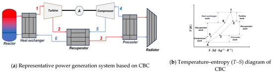
Figure 1.
Schematic diagrams of the power generation system based on CBC. (Numbers 1–6 indicate positions of system components: 1—turbine inlet, 2—turbine outlet, 3—precooler inlet, 4—compressor inlet, 5—compressor outlet, 6—heat exchanger inlet).
However, under conditions of load changes or external disturbances, the compressor operating point may approach or even cross the surge boundary. This unstable phenomenon can trigger flow separation, severe performance degradation, or mechanical damage [6,7]. Consequently, surge suppression and robust shaft speed regulation have become central challenges for ensuring CBC system stability, and developing effective anti-surge strategies remains a key research focus in this field.
Extensive studies have been carried out on the prevention of surge and the dynamic control of turbomachinery. Arnulfi et al. [8] conducted both numerical and experimental studies on surge instability in multi-stage compression systems and demonstrated the superior performance of high-gain feedback control based on performance map interpolation compared to passive methods. Sheng et al. [9] proposed a high-safety active/passive hybrid control strategy for centrifugal compressors, combining nonlinear model predictive control with flow estimation to enhance system robustness under actuator delays and dynamic uncertainties. Mousavi et al. [10] introduced a robust linear-matrix-inequality (LMI)-based model predictive control (MPC) scheme that considers actuator saturation and piping acoustic effects, effectively mitigating surge instability while maintaining low computational complexity. Schulze and Richter [11] developed a model-based MIN/MAX override control method for centrifugal compressors, integrating nonlinear output regulation and coverage control to ensure safe operation within the permissible operating range.
While these studies demonstrate the potential of advanced feedback and predictive control, most are validated under simplified or idealized conditions and rely heavily on accurate system models. Such dependence limits their adaptability to varying compressor architectures, operational disturbances, and real-world uncertainties. Moreover, extensive tuning is often required, reducing practical applicability. These limitations motivate the exploration of metaheuristic optimization algorithms, which can systematically enhance controller tuning and robustness, providing a natural transition to optimization-driven surge control strategies.
Metaheuristic optimization algorithms have been increasingly applied to enhance controller performance in surge prevention tasks. Li et al. [12] proposed a high-fidelity simulation framework for helium-xenon CBC systems in space nuclear applications, using NSGA-II to optimize startup control parameters and reduce energy demand, thereby addressing critical battery constraints in long-duration missions. Kail et al. [13] demonstrated improved frequency regulation in wind-integrated AGC systems using GA-optimized PID controllers. Naderi et al. [14] demonstrated enhanced dynamic performance and robustness in a 3-DOF helicopter system using a modified PSO (MPSO)-optimized adaptive fuzzy logic controller. While these studies effectively showcase the potential of metaheuristic algorithms in optimizing control performance, several limitations remain. For instance, NSGA-II and MPSO methods often involve high computational cost and require careful tuning of algorithm parameters, which can limit their real-time applicability in embedded or fast-response systems. Moreover, many of these works focus on system-level or simulation-based validation, with limited demonstration under varying operating conditions or practical constraints.
To address these challenges, the present study adopts a GA-based optimization strategy for PID controllers in CBC-based TAC systems subjected to load disturbances. A dynamic model is constructed in Simulink, with compressor surge boundaries identified using characteristic performance curves. The PID controller gains are optimized using a genetic algorithm based on a weighted fitness function incorporating overshoot, rise time, and integral of absolute error, systematically balancing multiple control objectives. The originality of this approach lies in integrating metaheuristic optimization directly with PID control specifically tailored for surge prevention in CBC systems. Unlike conventional PID tuning, which relies on empirical adjustment and other metaheuristic methods, GA-PID achieves both high computational efficiency and practical implementability in real-time applications. Furthermore, unlike classical anti-surge strategies that depend primarily on hardware modifications or simple feedback schemes, this approach directly optimizes the control law, significantly enhancing the closed-loop dynamic response of the compressor. Simulation results validate the method’s effectiveness in improving dynamic stability and preventing surge under complex disturbance conditions. It should be noted that the present study is based on simulation experiments and does not take into account pressure and temperature losses in piping connections or actuator wear, as is commonly performed in similar studies [15,16].
2. System Description
Although the CBC operates as a tightly coupled system composed of multiple interdependent components, the operational stability of the compressor plays a critical role in determining the system’s overall dynamic performance, especially under transient disturbances that can lead to surge. While a complete system model would involve multiple heat exchangers, flow paths, and control loops, this study focuses specifically on the core TAC unit. By constructing a high-fidelity dynamic model of the TAC subsystem, the research isolates and investigates the dynamic behavior and surge risk of the compressor under load disturbances.
In addition, the choice of working fluid significantly influences thermodynamic performance and control sensitivity. Based on prior studies concerning thermal properties and system compatibility, a He–Xe mixture with a molar mass of approximately 40 g/mol is selected. This blend provides a balance between high thermal conductivity and appropriate gas density, establishing a consistent thermophysical foundation for accurate modeling and simulation (calculation method shown in Appendix A) [17,18,19,20].
2.1. TAC System
The TAC system, an integrated unit comprising the turbine, alternator, and compressor, serves as the core component of the space-based closed Brayton cycle. Through a tightly coupled mechanical structure, it transmits mechanical power from the turbine directly to the compressor while simultaneously driving the alternator for electrical energy conversion. The TAC system is characterized by its compact configuration, high mechanical transmission efficiency, and rapid dynamic response, making it a critical enabler for efficient and stable operation in closed-loop Brayton cycle systems [21,22,23]. The subsequent sections provide a detailed description of the turbine, compressor, and rotor models.
2.1.1. Turbine Model
The turbine functions as a key component for converting the thermal energy of high-temperature, high-pressure He–Xe working fluid into mechanical work. In operation, the He–Xe gas absorbs heat from the nuclear reactor, increasing its temperature and pressure before entering the turbine. Inside the turbine, the gas undergoes expansion, transforming thermal energy into shaft work to drive the rotor. A multi-stage turbine configuration is commonly employed to enhance energy conversion efficiency. Turbine blades are typically fabricated from high-temperature-resistant and high-strength materials to ensure reliable operation under extreme thermal and pressure conditions. The thermodynamic expansion process corresponds to the expansion stage on the T–S diagram, as illustrated in Figure 1b. Under ideal conditions, the turbine outlet temperature can be estimated using the following equation:
where is the ratio of specific heat, is the adiabatic index, and is the expansion ratio. The value of can be determined based on the pressure losses across various components and the pressure ratio of the compressor. It is calculated using the following equation:
During the expansion process in the turbine, the isentropic efficiency of the turbine represents the ratio of the actual work output during the expansion process to the ideal work output under isentropic conditions:
Based on this equation, the actual outlet temperature can be derived as follows:
Owing to the significant nonlinear behavior exhibited by compressors and turbines during real-world operation—especially under extreme conditions such as high pressure ratios and low mass flow rates—their characteristics cannot be accurately captured using simplified theoretical models. As a result, reliable performance maps derived from experimental measurements or high-fidelity simulations are essential for describing their operating behavior with sufficient precision [16].
In this study, the adopted characteristic curves are referenced from the 132 kWe CBC Turbo-Compressor description in the literature [24]. This reference provides polynomial fitting formulas relating turbine pressure ratio, temperature ratio, and mass flow rate at various shaft speeds (with a design speed of 59,850 rpm). However, according to the simulation requirements of this study, the characteristic curve of mass flow rate needs to be derived. Hence, the mass flow rate must be inversely calculated from the expansion ratio. The calculated turbine characteristic curve is shown in Figure 2.
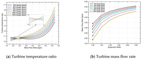
Figure 2.
Characteristic curve of the turbine.
The output power of the turbine is calculated using the average specific heat at constant pressure, as given by the following equation:
In this study, the turbine module was constructed in Simulink based on the above principles, as shown in Figure 3, and serves as the foundation for subsequent experiments.
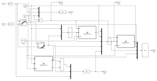
Figure 3.
Turbine schematic diagram constructed in Simulink.
2.1.2. Compressor Model
The compressor is responsible for compressing the low-temperature, low-pressure He–Xe gas mixture, raising its pressure to enable reheating in the reactor. During the compression process, both the temperature and pressure of the working fluid increase significantly. This process corresponds to the compression stage on the cycle’s T–S diagram. Under ideal conditions, the outlet temperature of the compressor, denoted as , can be calculated using the following equation:
In the process of the compressor, the isentropic efficiency () represents the ratio of the ideal compression work to the actual compression work, and is defined as follows:
Based on this equation, the actual outlet temperature can be derived as follows:
The characteristic curves of the compressor’s pressure ratio and temperature ratio are also obtained from the literature [24], as shown in Figure 4.
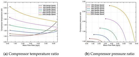
Figure 4.
Characteristic curve of the compressor.
Similar to the turbine, the isentropic efficiency of the compressor is determined based on the relationship between the pressure ratio and the temperature ratio, as given by the following equation:
is derived as follows:
The output power of the compressor is calculated by the following formula:
As shown in Figure 5, the Simulink model of the compressor can also be used as the foundation for further experimental studies.
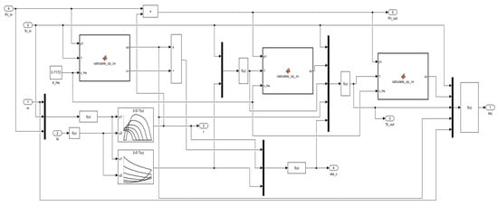
Figure 5.
Compressor schematic diagram constructed in Simulink. ( —compressor inlet temperature, —compressor outlet temperature, —compressor inlet pressure, —compressor outlet pressure, —compressor efficiency).
2.1.3. Rotor Model
In the TAC model, the turbine, alternator, and compressor are mounted on a common shaft. Therefore, dynamic analysis must account for the interactions among the shaft rotational speed , rotor moment of inertia , and the mechanical loads imposed by each component.
The surplus power on the TAC shaft can be expressed as follows. This equation represents the power balance within the TAC system, where the shaft surplus power () is defined as the difference between the expansion power produced by the turbine and the power consumed by both the compressor and the alternator load:
The TAC rotor model combines the surplus power with the corresponding shaft torque to determine the rate of change of shaft speed, which can be expressed by the following equation:
When , the shaft speed remains constant. If , increases; conversely, it decreases. Under steady-state conditions, the turbine expansion power must equal the sum of the compressor power consumption and the generator load, which means . According to the above description, the rotor model can be constructed in Simulink, as shown in Figure 6.
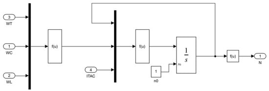
Figure 6.
Rotor schematic diagram constructed in Simulink. (ITAC—rotor moment of inertia).
2.2. TAC Model Validation
In this study, each model is independently constructed based on its thermodynamic cycle, and pressure and temperature losses due to piping are neglected. The constructed TAC unit model is illustrated in Figure 7. Given the limited availability of theoretical and experimental data on space Brayton cycles, this model adopts key design parameters from the final report of the SP-100 program, issued by the U.S. Department of Energy in 1983 [25]. By applying the same boundary and decision conditions as the SP-100 scheme and performing thermodynamic calculations using the proposed TAC model, the key simulation results were compared with SP-100 benchmark data to validate the model’s accuracy. As shown in Table 1, the maximum temperature deviation across nodes is 2.23%, and the maximum pressure deviation is 1.16%. The calculated results show good agreement with the SP-100 reference values, with deviations within acceptable limits, thereby confirming the reliability of the proposed model.
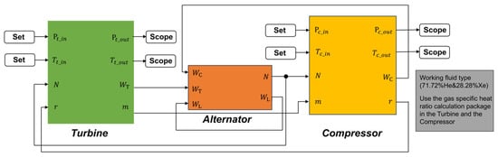
Figure 7.
TAC model schematic diagram.

Table 1.
Comparison of cycle node temperatures and pressures with the SP-100 program.
To further validate the reliability of the developed TAC model, this study incorporates additional reference data from the literature, as shown in Table 2, and presents a systematic comparison in Figure 8 [16,22,26]. The simulated results show close agreement with the design values, with relative errors generally below 4%. For example, the turbine inlet temperature of 1500 K is only 1.44% lower than the design value (1522 K), and the turbine outlet temperature of 1165.3 K closely matches the reference (1163 K). Pressure characteristics are also consistent, with deviations within 4%. In comparison, Reference [18] reports a lower turbine inlet temperature (1153 K) and much lower alternator power (161 kW), whereas Reference [23] adopts a higher pressure regime (3.30 MPa) and reports a lower alternator power (273 kW) than the present simulation (1000.44 kW). These differences likely result from simplified component modeling and conservative design assumptions in the literature, which limit system-level comparison. In contrast, the present work provides a more physically consistent and comprehensive dataset, achieving highly accurate turbine, compressor, and alternator powers (errors < 1%) and exactly reproducing the shaft speed of 55,000 rpm, thereby confirming the robustness of the proposed model in thermophysical coupling and component matching.
Table 2.
Comparison of simulation results with design values.
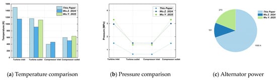
Figure 8.
Compared with existing studies. (References shown in the figure are: Wu.Z. 2024 corresponds to [22], Wu.Y. 2025 corresponds to [26]).
3. Challenges and Solutions
3.1. Load Disturbance During TAC Model Operation
During the development of the TAC model, the rotor model introduced the key variable of excess power () and established the relationship among rotor speed, shaft torque, and excess power. Under steady-state conditions, the power output of the turbine must balance the power consumed by the compressor and the generator load (), and the rotor speed remains constant. When the system load decreases, the excess power becomes positive (), increasing shaft speed. Conversely, an increase in system load leads to negative excess power () and a corresponding decrease in rotor speed [16,27]. By introducing a step disturbance in the system load, the resulting rotor shaft speed variation is analyzed, as illustrated in Figure 9. The magnitude and duration of the step load disturbance are adopted from Reference [16]. Although the reference does not explicitly confirm whether these disturbances represent real-world operating conditions, they are sufficient to induce measurable rotor speed variations, allowing evaluation of the system’s dynamic response and the proposed control strategy.
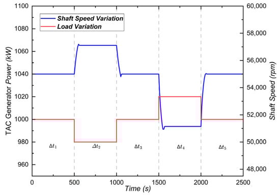
Figure 9.
Manual load and shaft speed variations.
Under a load reduction disturbance introduced at 500 s, the excess power becomes negative. As a result of the rotor’s feedback mechanism, the shaft speed increases from 55,000 rpm and eventually stabilizes at 57,111 rpm. When the load returns to its initial level at 1000 s, the excess power turns positive, causing the rotor speed to decrease and settle back to the original 55,000 rpm. At 1500 s, an increase in load results in positive excess power, leading to a decrease in rotor speed, which eventually stabilizes at 50,610 rpm. Finally, the load returns to its initial level again at 2000 s, and the shaft speed settles back to the original 55,000 rpm. These results indicate that under load reduction, the dynamic steady-state point shifts to a higher rotor speed range, while under load increase, it shifts to a lower speed range.
In Brayton cycle systems, the alternator typically operates under complex conditions with frequent external disturbances, leading to unpredictable load fluctuations. These disturbances disrupt the internal power balance and result in rotor shaft speed variations. Such speed changes not only characterize the system’s dynamic response but may also impair the matching between the compressor and turbine. If not properly controlled, these mismatches can trigger compressor surge, posing a serious threat to overall system stability [28,29,30].
Surge is a low-frequency, high-amplitude aerodynamic oscillation that can cause severe damage to the compressor. In aerospace applications, where reliability and safety are of paramount importance, surge avoidance is essential. By analyzing compressor characteristic curves at various shaft speeds, the surge line can be identified. This line serves as a reference for defining the surge margin and designing control strategies to ensure the system operates within stable boundaries [31,32,33].
To ensure operational safety while avoiding overly conservative constraints, the surge margin threshold was set to 0.20 in this study. This value corresponds to a 20% margin between the current operating point and the surge line on the compressor characteristic curve, as defined by the following:
In compressor modeling and control strategy design, accurately identifying the surge point is essential to maintaining system stability. The surge point has a clear physical interpretation on the compressor performance map and can be determined from experimental or simulated performance curve data using interpolation or curve-fitting techniques under various operating conditions. Specifically, for a given set of performance curves, the data are grouped by rotational speed, and for each speed, the minimum stable mass flow rate is identified as the corresponding surge point. By connecting the surge points across different speed levels, a complete surge line can be constructed. This method applies to performance maps obtained through experimental measurements. The surge line derived from the pressure ratio performance curves used in this study is illustrated in Figure 10.
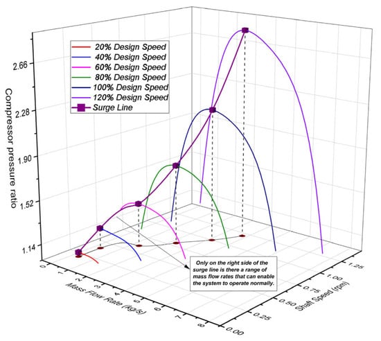
Figure 10.
Characteristic curves of compressor pressure ratio with surge line.
As shown in Figure 11a, large load variations can lead to significant fluctuations in rotor shaft speed, potentially causing the compressor to exit its stable operating region and enter the surge zone. Under such conditions, the compressor operating point approaches or even crosses the surge line on the performance map, posing a considerable risk of aerodynamic instability, as shown in Figure 11b. This may result in severe flow oscillations and pressure fluctuations, which could lead to mechanical damage to critical system components.
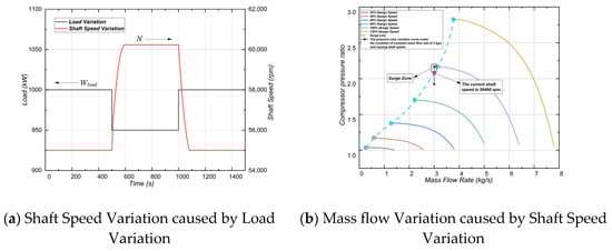
Figure 11.
Load variation causes mass flow to enter the surge region.
3.2. Control Model
To mitigate the uncertainties introduced by load disturbances, this study proposes a combined control scheme that integrates bypass valve regulation with shaft speed control. The objective is to enhance the system’s disturbance rejection capability and maintain stable operation with a sufficient margin from the surge boundary [34].
The control model operates in two stages:
- (1)
- The bypass valve control logic continuously monitors the system state. When the operating point is detected to be approaching the surge region, the bypass valve is promptly actuated to open, thereby diverting a portion of the flow. This adjustment increases the total mass flow rate through the compressor, rapidly shifting the operating point away from the surge boundary and restoring system stability.
- (2)
- The speed control model subsequently engages to adjust the target shaft speed of the alternator rotor, compensating for the dynamic deviations induced by the disturbance. This control action enhances the system’s recovery rate and improves steady-state accuracy, thereby reinforcing overall operational stability.
3.2.1. Bypass Valve Control
In the Brayton cycle system established in this study, the bypass valve is positioned between the turbine outlet and the compressor inlet, forming a recirculation loop. This configuration facilitates rapid adjustment of the working fluid parameters at the compressor inlet; however, since this research focuses on a detailed analysis of the TAC unit, variations in pressure and temperature at the compressor inlet due to working fluid changes are not considered [35]. The mass flow rate passing through the bypass valve is as follows:
is the valve opening parameter, which is regulated by a PI controller:
The error function is expressed as follows:
When a sudden load disturbance occurs, the compressor speed increases, resulting in a higher pressure ratio and reduced mass flow, which pushes the operating point toward the surge line and risks entering an unstable region. To prevent this, the bypass valve is automatically actuated based on real-time mass flow measurements. Once the surge margin falls below a predefined threshold, the valve opens to recirculate part of the flow, thereby restoring the operating point to a stable region.
3.2.2. Shaft Speed Control
The primary function of the shaft speed control model is to regulate the alternator’s output power in real time based on the deviation between the current system state and the desired operating condition. This facilitates rapid recovery to steady-state operation and improves overall system stability and disturbance tolerance.
A PID control strategy is implemented, where the controller computes the control signal based on the error between the reference and actual shaft speeds. This signal is subsequently used to adjust the rotor power accordingly.
The characteristic curve of the compressor reveals the nonlinear coupling relationship among the mass flow rate , pressure ratio , and rotational shaft speed , as expressed by the following equation:
Based on this equation, the mass flow rate can be derived as follows:
By monitoring the compressor outlet pressure and shaft speed in real time, the corresponding mass flow rate can be determined. This real-time mass flow is then compared with the reference mass flow () at a given reference speed (). If the current mass flow falls within a predefined danger zone, the speed control mechanism is activated. A PID controller is employed to generate the control signal, enabling dynamic adjustment of the shaft speed to ensure safe and stable system operation:
The is combined with the disturbance introduced by the rotor, serving as an auxiliary input in regulating the shaft speed. Through this speed control model, the compressor’s operating conditions can be dynamically adjusted under varying load disturbances. Figure 12 shows the schematic diagram of the TAC system after the addition of the bypass valve model and the shaft speed control model.
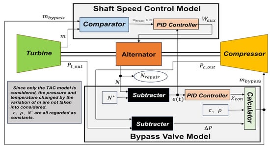
Figure 12.
Bypass valve control and shaft speed model execution diagram.
4. Results and Discussion
4.1. Selection of PID Parameters
Within this framework, the PID controller is utilized to regulate both the shaft speed and the mass flow rate. Its performance directly influences the system’s capability to suppress disturbances and restore the desired operating conditions. Given the highly nonlinear and coupled nature of compressor dynamics, the selection of PID parameters plays a critical role in determining controller effectiveness. Improper tuning may lead to sluggish responses, oscillations, or even system instability. Therefore, targeted optimization of PID parameters, tailored to system characteristics and control objectives, is of substantial theoretical significance and practical relevance for ensuring the stable operation of the Brayton cycle system.
4.1.1. Method of Selecting Parameter
To address control challenges under load disturbances in the Brayton cycle system, this study employs a GA to optimize PID controller parameters. GA is well-suited to the established TAC model with clear transient and steady-state behaviors [36,37,38,39,40], enabling efficient offline search for optimal PID gains through a composite performance index.
Alternative control techniques, such as neural networks, adaptive control, and Model Predictive Control (MPC), were considered. Neural networks provide nonlinear processing and self-learning capabilities, but their practical application in Brayton systems is limited by the scarcity of high-quality training data, potential overfitting, and high computational overhead for real-time operation. Adaptive control, although theoretically suitable for time-varying systems, may face challenges related to observability, stability, and tuning complexity in highly coupled dynamic environments like TAC systems. MPC can explicitly handle constraints and anticipate future disturbances, yet it requires accurate system modeling and significant computational resources, which may hinder its implementation in complex energy systems. In contrast, the GA offers a simpler, more robust, and practically feasible approach for tuning PID parameters under these constraints, balancing control performance, computational efficiency, and implementation complexity.
During the optimization process, GA searches for the optimal set of proportional ), integral (), and derivative () gains, thereby enhancing both transient response and steady-state accuracy. The specific process of obtaining PID parameters using GA is shown in Figure 13. The relevant parameters for the PID parameter tuning in this study are shown in Table 3. The GA parameters were selected with reference to existing studies on GA-based control optimization [38,41]. These settings were chosen to balance convergence speed and solution diversity, thereby enhancing the robustness and reliability of the tuning process.
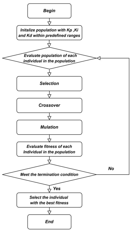
Figure 13.
GA flowchart.
Table 3.
The relevant parameters for the PID parameter tuning.
4.1.2. PID Parameter Results
To accurately evaluate the performance of the PID controller, the fitness function is designed to capture both the dynamic and steady-state characteristics of the system. Specifically, rise time, overshoot, and integral of absolute error are selected as key performance indicators. Rise time characterizes the system’s response speed, overshoot quantifies the maximum deviation during the transient phase, and the integral of absolute error measures the final deviation from the desired value. These metrics are particularly critical for the TAC system, as excessive overshoot or error may shift the compressor operating point into the surge region, thereby undermining system stability. By adjusting the control parameters of both the speed controller and the bypass valve, the genetic algorithm seeks to minimize these indices and ensure a fast and stable system response.
The fitness function is constructed as a weighted sum of the normalized performance indices:
where , and are the weight coefficients for , and respectively.
Table 4 presents several sets of optimized PID parameters with their corresponding fitness values under different weight combinations, together with one set of manually tuned PID parameters. These control groups are entirely part of our own experimental design and are not derived from existing literature. Specifically, we selected multiple weight ratios in the fitness function to represent both balanced and biased preferences among the performance indices, while the manually tuned parameters were obtained through iterative step-response tests at the nominal setpoint and further refined under ±5% target power variations. Each candidate configuration (manual and weighted-sum optimized) was then evaluated at three target power levels—500 kW (nominal), 475 kW (−5%), and 525 kW (+5%). Figure 14 illustrates the corresponding dynamic responses, showing that the PID controller maintains consistent performance across all setpoints, with fast response, minimal overshoot, and good steady-state accuracy. Comparison of the scalar fitness values, computed as a weighted sum of normalized time-domain indices, indicates that the weight setting consistently yields the best overall trade-off between dynamic speed and stability, and is therefore adopted in this study.
Table 4.
PID parameters and fitness function values at the target value and ±5% deviation.
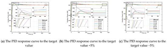
Figure 14.
PID response curves under target value and ±5% deviation.
To further validate the stability of the proposed PID control strategy, a Lyapunov function: ; its derivative is . By substituting the PID control law Equation (20) into the derivative of the Lyapunov function, we obtain the following:
With appropriately selected PID parameters, the derivative of the Lyapunov function satisfies , indicating that the closed-loop system is stable in the Lyapunov sense and that the speed error converges to zero over time. Simulation results in this study show that the Lyapunov function derivative remains non-positive for all optimized PID parameters, confirming system stability and providing theoretical support for the GA-optimized PID design.
Notably, the GA-PID controller adjusts parameters solely based on the target value and the current output, without requiring an exact physical model. This feature inherently provides robustness against model uncertainties and minor component degradation.
The proposed GA-PID control strategy is implemented as a combined bypass valve and rotor speed control scheme in the TAC model to mitigate load disturbances and prevent surge. To realize this in practice, rotor speed measurements require a sampling frequency of 100 Hz with an accuracy of ±0.5% of the rated speed, and the bypass valve actuator should have a response time of approximately 0.2 s to promptly adjust mass flow (based on typical industrial hardware specifications). The GA optimization is performed offline, and only the resulting PID law is executed online, imposing minimal computational demand. Consequently, the GA-PID controller can regulate rotor speed in real-time within the TAC system and is fully compatible with embedded platforms commonly used in CBC plants, such as PLCs, DSPs, or industrial PCs.
4.1.3. Comparison with Other Optimization Methods
To further assess the effectiveness of the proposed GA-PID controller, comparative simulations were conducted using PID controllers optimized with Particle Swarm Optimization (PSO) and Differential Evolution (DE), alongside the conventional manually tuned PID. All controllers were evaluated under identical TAC system scenarios, with the target power level set at 500 kW (nominal). Performance metrics were calculated and normalized with respect to the conventional PID results for direct comparison. To facilitate understanding of the simulation setups, Figure 15 illustrates the control framework of the GA-PID, PSO-PID, DE-PID, and conventional PID controllers in Simulink.
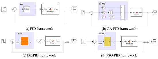
Figure 15.
Simulation framework of the four PID optimization methods.
The normalized performance metrics are summarized in Table 5. The GA-PID consistently demonstrates superior trade-offs among dynamic response, overshoot, and steady-state accuracy compared to both PSO-PID and DE-PID. While PSO and DE improve certain individual indices, GA-PID achieves the best overall balance across all key performance indicators, highlighting the effectiveness of the GA-based multi-objective tuning approach. It is worth noting that although NSGA-II is a widely used multi-objective optimization algorithm, it was not employed in this study due to its relatively high computational complexity and implementation overhead for the TAC system. The single-objective GA with a weighted-sum fitness function was sufficient to achieve a balanced improvement in rise time, overshoot, and steady-state error, meeting the system performance requirements.
Table 5.
Normalized performance comparison of different PID optimization methods.
These results indicate that the GA-PID controller provides a more balanced improvement across all performance indicators, ensuring both rapid transient response and accurate steady-state behavior. The normalized table clearly demonstrates the advantages of GA-based optimization over other commonly used metaheuristic methods in TAC systems.
4.2. Robustness Analysis of the Control Model
To evaluate the practical applicability and robustness of the proposed GA-optimized PID controller, additional simulations were conducted considering parameter uncertainties, compressor map variations, and sensor noise. These experiments are intended to assess the controller’s behavior under more realistic, non-ideal conditions. It should be noted, however, that the results are still based solely on numerical simulations.
4.2.1. Parameter Uncertainty Analysis
A parameter uncertainty analysis was carried out by perturbing the bypass valve opening coefficient, which was chosen as the representative tunable parameter in the TAC model. The coefficient was varied by ±5% and ±10% to investigate how this uncertainty affects closed-loop system performance. The simulation outcomes, summarized in Table 6, show that the system remains stable in all cases, with only moderate variations in overshoot, settling time, and steady-state error. These results suggest that the proposed PID controller exhibits satisfactory robustness against deviations in the bypass valve characteristics, which are likely to occur in practice.
Table 6.
System performance under bypass valve disturbances.
4.2.2. Compressor Map Variation Analysis
To examine the influence of deviations in compressor characteristics, which may arise from manufacturing tolerances or long-term degradation, the nominal compressor map was modified by ±5% in both pressure ratio and mass flow. The GA-optimized PID controller was then tested under the same step load disturbances. As presented in Table 7, the controller successfully stabilized the system despite the altered compressor maps, with only slight differences in the key performance indices compared to the nominal case. These results demonstrate that the controller maintains effective performance even when the compressor operating map shifts within realistic bounds.
Table 7.
System performance under compressor map variations.
4.2.3. Sensor Noise Analysis
To assess the robustness of the controller to measurement inaccuracies, Gaussian white noise with standard deviations of 1%, 3%, and 5% of the signal range was injected into the rotational speed and pressure signals. The system was simulated under identical disturbance conditions using the GA-optimized PID controller. As shown in Table 8, although the presence of noise slightly increases overshoot and settling time, the closed-loop system remains stable, and the overall performance degradation is limited. This indicates that the proposed controller can tolerate realistic sensor noise levels while still ensuring reliable operation.
Table 8.
System performance under sensor noise disturbances.
4.3. Optimization Results of the Control Model
To validate the effectiveness of the proposed PID control model optimization strategy under realistic operating conditions, multiple types of load disturbances were introduced into the TAC Brayton cycle system model, and the system responses before and after optimization were comparatively analyzed. Specifically, a complete steady-state TAC model was constructed in the Simulink environment, and three representative disturbances were applied to the rotor model: larger linear disturbances, smaller linear disturbances, and nonlinear disturbances, as illustrated in Figure 16. These disturbances were designed to simulate various dynamic variations induced by different types of sudden load fluctuations.
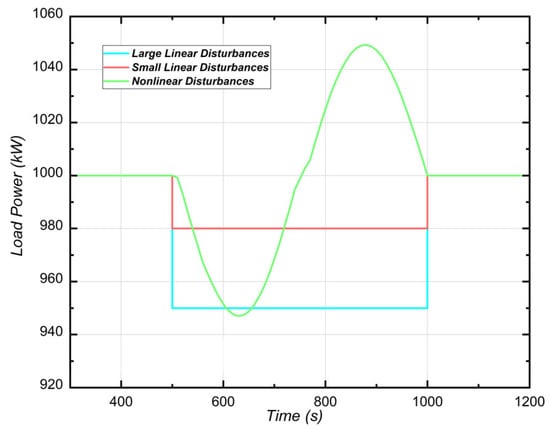
Figure 16.
Manually tuned load disturbances.
Figure 17 illustrates the variations in rotor shaft speed and mass flow rate under three representative load disturbances without any control mechanisms applied. In contrast, Figure 18 demonstrates the system response after implementing the proposed control strategy. Under large linear disturbances, a significant fluctuation in mass flow rate occurs at 513 s, indicating that the system approaches the surge boundary. In response, the bypass valve control module is immediately activated to regulate the working fluid flow, allowing the mass flow rate to quickly stabilize according to the demand dictated by the current shaft speed. Conversely, under small linear and nonlinear disturbances, the mass flow rate exhibits negligible variations throughout the simulation. Since the oscillation threshold defined in this study was not exceeded, the inherent adjustment mechanism of the rotor model was sufficient to restore the original speed. Consequently, the proposed control module was not required in these scenarios. These findings suggest that the proposed control strategy is particularly effective in mitigating large disturbances, where it plays a crucial role in preventing surge and maintaining stable speed regulation. Thus, its primary application scope encompasses scenarios involving significant load fluctuations.
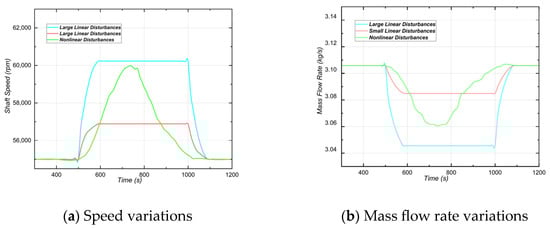
Figure 17.
Shaft speed and mass flow rate responses under load disturbances.
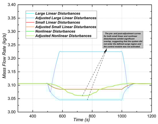
Figure 18.
Mass flow rate after the bypass valve.
Figure 19 compares the load and shaft speed responses under three control strategies: no control, PID control, and GA-PID optimization. Due to the activation of the bypass valve, both PID and GA-PID schemes initiate regulation immediately after the load disturbance at 513 s. In contrast, the uncontrolled system lacks such corrective measures. The subsequent shaft speed recovery behavior shows a significant improvement with advanced control. Specifically, the recovery time required for the rotor speed to return to its nominal level was 1080 s without control, reduced to 752 s with PID control, and further shortened to 680 s using the GA-PID strategy. These results demonstrate the superior responsiveness and disturbance rejection capability of the GA-PID controller compared to PID, particularly under transient load conditions.
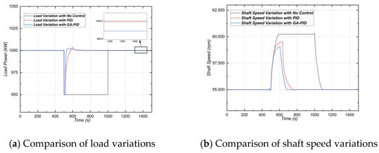
Figure 19.
Load variation and rotor shaft speed variations diagram.
As shown in Table 9, the GA-PID controller reduced the settling time from 567 s (no control) to 167 s, representing a 70.6% decrease compared to the uncontrolled case and a 30.1% decrease compared to conventional PID control. The overshoot peak decreased from 3.5805 kW to 2.3051 kW, corresponding to a 35.6% reduction. During steady-state operation, the system maintained a surge margin of 0.256, which is 37.6% higher than the uncontrolled case and equal to that of PID control, effectively avoiding instability and ensuring safe operation under varying load conditions.
Table 9.
The differences in the impact of without control, PID, and GA-PID tuning on the system.
4.4. Prospects and Future Work
The proposed framework, which combines GA-based PID optimization with coordinated dual-model regulation, significantly enhances dynamic response, surge margin, and disturbance rejection. The results suggest substantial potential for deployment in advanced high-performance energy conversion systems, particularly CBC architectures. Potential applications include aerospace propulsion systems, where the controller can help maintain rotor speed stability under varying thrust demands; space-based nuclear power units, where reliable surge prevention and automatic disturbance rejection are critical for long-duration autonomous operation; and industrial CBC implementations, where the controller can optimize load-following performance and enhance operational safety.
Although effective under step load disturbances, the controller has not been tested under rapid or stochastic disturbances. Future work will focus on experimental validation using a physical test rig to verify the controller’s performance in real hardware conditions, as well as real-time implementation studies on embedded platforms to evaluate computational requirements, sampling rates, and actuator limitations. Currently, the proposed GA-PID-based anti-surge control framework has been validated only for the CBC system. While it has not yet been applied to other thermodynamic cycles, such as Rankine or Organic Rankine Cycles (ORCs), the core optimization framework and coordinated control strategy are fundamentally general. Adapting the methodology to these systems would require corresponding system modeling and parameter tuning. In addition, the framework will be further extended to different CBC architectures, various working fluids, and more complex disturbance scenarios. Further investigations will also consider model uncertainties, long-term component degradation, actuator wear, and integrate system efficiency and energy consumption through thermodynamic modeling and multi-objective optimization to provide a comprehensive assessment for practical deployment.
5. Conclusions
To enhance the operational stability and control performance of the closed Brayton cycle TAC system under load disturbances, this study conducted a comprehensive investigation focusing on system modeling, controller design, and parameter optimization. The main contributions of this work are summarized as follows:
- (1)
- A high-fidelity steady-state model of the TAC-based closed Brayton cycle system was developed in the Simulink environment. This model incorporates key components, including the compressor, turbine, and alternator rotor, and serves as a reliable platform for analyzing system dynamics under both nominal and disturbed conditions.
- (2)
- To overcome the limitations of conventional PID controllers, such as sluggish response, excessive overshoot, and Integral of absolute error, a multi-objective performance index was formulated by integrating rise time, overshoot, and Integral of absolute error deviation. GA was employed to globally optimize the PID parameters. The optimized controller achieved a 70% improvement in rotational speed regulation performance, significantly enhancing dynamic responsiveness and control precision.
- (3)
- A dual-control strategy was implemented by integrating a shaft speed control model with a bypass valve control model. This coordinated control approach enables real-time adjustment of both shaft speed and mass flow rate. Simulation results confirm that the proposed method effectively mitigates system oscillations, ensures rapid system recovery, and maintains the compressor operating point consistently outside the surge region throughout the entire disturbance scenario.
Author Contributions
Conceptualization, H.L., X.T. and Q.N.; methodology, H.L., X.T. and Y.S.; software, H.L. and Y.S.; validation, Q.F., F.H. and J.Y.; resources, Q.N.; writing—original draft preparation, writing—review and editing, H.L. All authors have read and agreed to the published version of the manuscript.
Funding
This work is financially supported by the National Natural Science Foundation of China (Grant No. 62373262).
Data Availability Statement
The data presented in this study are available on request from the corresponding author due to privacy.
Conflicts of Interest
No conflicts of interest exist in the submission of this manuscript, and the manuscript is approved by all authors for publication. I declare on behalf of my co-authors that the work described herein is original research that has not been published previously, and is not under consideration for publication elsewhere, in whole or in part.
Nomenclature
| Temperature, [] | |
| Entropy, [] | |
| Pressure, [] | |
| Heat capacity at constant pressure, [] | |
| Average heat capacity at constant pressure from i to j, [] | |
| Heat capacity at constant volume, [] | |
| Turbine inlet temperature, [] | |
| Turbine outlet temperature, [] | |
| Ideal turbine outlet temperature, [] | |
| Compressor inlet temperature, [] | |
| Compressor outlet temperature, [] | |
| Ideal compressor outlet temperature, [] | |
| Turbine inlet pressure, [] | |
| Turbine outlet pressure, [] | |
| Ideal turbine outlet pressure, [] | |
| Compressor inlet pressure, [] | |
| Compressor outlet pressure, [] | |
| Ideal compressor outlet pressure, [] | |
| Pressure ratio | |
| Expansion ratio | |
| Ratio of specific heat | |
| Adiabatic index | |
| Average pressure loss ratio from i to j | |
| Isentropic efficiency of the turbine | |
| Isentropic efficiency of the compressor | |
| Turbine output power, [] | |
| Compressor output power, [] | |
| Load power, [] | |
| Excess power, [] | |
| Auxiliary power, [] | |
| m | Mass flow rate, [] |
| Mass flow rate under safe operating conditions, [] | |
| N | Rotor shaft speed, [] |
| Rotor shaft speed under safe operating conditions, [] | |
| Rotational moment of inertia for the TAC and shaft, [] | |
| Bypass valve opening parameter | |
| Density of the working fluid, [] | |
| Bypass valve coefficient | |
| Shaft speed model coefficient | |
| Integral of absolute error | |
| Rise time | |
| Overshoot | |
| Surge margin threshold | |
| Current mass flow rate, [] | |
| Mass flow rate at the surge line, [] | |
| Pressure difference across the bypass valve, [] |
Abbreviations
The following abbreviations are used in this manuscript:
| CBC | Closed Brayton Cycle |
| TAC | Turbine–Alternator–Compressor |
| GA | Genetic Algorithm |
| PID | Proportional-Integral-Derivative |
Appendix A
Appendix A.1. Virial Coefficient of He-Xe Mixture
Expression of the ideal gas equation:
Based on the ideal gas equation, the compressibility factor is introduced to account for the deviation of real gases from ideal behavior. It is defined as the ratio of the molar volume of a real gas to that of an ideal gas []. The value of typically approaches 1. By adding a series expansion to further correct for non-ideal behavior, the equation evolves into the Virial equation.
General form of the Virial equation:
In principle, the expressions for each Virial coefficient can be theoretically derived, but in practice, calculating higher-order Virial coefficients is extremely difficult. Except for simple hard-sphere models, only the third Virial coefficient can typically be computed. As a result, Virial coefficients are usually determined experimentally. Therefore, the compressibility factor expanded to the third-order Virial form is:
The second-order Virial coefficient B for a mixture of gases is calculated as follows:
is the second-order Virial coefficient of helium, is the second-order Virial coefficient of xenon, is the second-order cross Virial coefficient for the He-Xe gas mixture.
where and represent the characteristic molar volumes of xenon and the He-Xe gas mixture, respectively, while and denote the reduced temperatures of xenon and the He-Xe gas mixture, respectively. For the third-order Virial coefficient of the gas mixture, its calculation follows the same approach as that of the third-order Virial coefficients of helium and xenon:
where is the third-order Virial coefficient of helium, is the third-order Virial coefficient of xenon, and and are the third-order cross Virial coefficients of the He-Xe gas mixture. The relations are given by and .
Appendix A.2. Specific Heat Capacity of He-Xe Mixture
The molar specific heat at constant pressure and the molar specific heat at constant volume are calculated using the following formulas:
References
- Ayodele, O.L.; Luta, D.N.; Kahn, M.T. A Micro-Nuclear Power Generator for Space Missions. Energies 2023, 16, 4422. [Google Scholar] [CrossRef]
- Ashe, T.L.; Baggenstoss, W.G.; Bons, R. Nuclear Reactor Closed Brayton Cycle Power Conversion System Optimization Trends for Extra-Terrestrial Applications. In Proceedings of the 25th Intersociety Energy Conversion Engineering Conference, Reno, NV, USA, 12–17 August 1990; Volume 1, pp. 125–134. [Google Scholar]
- El-Genk, M.S. Space Nuclear Reactor Power System Concepts with Static and Dynamic Energy Conversion. Energy Convers. Manag. 2008, 49, 402–411. [Google Scholar] [CrossRef]
- Cheng, K.; Li, J.; Yu, J.; Qin, J.; Jing, W. Dynamic Characteristics Analysis for a Novel Double-Rotor He-Xe Closed-Brayton-Cycle Space Nuclear Power Generation System. Energies 2023, 16, 6620. [Google Scholar] [CrossRef]
- Chen, W.; Song, M.; Qian, Y.; Yu, H.; Yan, J. Research and Development of Helium-Xenon Brayton Cycle Technology: A Review. Natl. Sci. Open 2024, 3, 20230089. [Google Scholar] [CrossRef]
- Greitzer, E.M. Surge and Rotating Stall in Axial Flow Compressors—Part I: Theoretical Compression System Model. J. Eng. Power 1976, 98, 190–198. [Google Scholar] [CrossRef]
- Lang, L.; Jiang, F.; Cheng, K.; Liu, Z.; Wang, S.; Dang, C.; Qin, J.; Huang, H.; Zhang, X. Dynamic Characteristics Analysis of Supercritical CO2 Closed Brayton Power Generation System for Hypersonic Vehicles. Appl. Therm. Eng. 2025, 269, 126016. [Google Scholar] [CrossRef]
- Arnulfi, G.L.; Blanchini, F.; Giannattasio, P.; Micheli, D.; Pinamonti, P. Extensive Study on the Control of Centrifugal Compressor Surge. Proc. Inst. Mech. Eng. Part A J. Power Energy 2006, 220, 289–304. [Google Scholar] [CrossRef]
- Sheng, H.; Chen, Q.; Zhang, J.; Zhang, T. A High-Safety Active/Passive Hybrid Control Approach for Compressor Surge Based on Nonlinear Model Predictive Control. Chin. J. Aeronaut. 2023, 36, 396–412. [Google Scholar] [CrossRef]
- Mousavi, H.; Nekoui, M.A.; Derakhshan, G.; Hakimi, S.M.; Imani, H. A Novel Robust MPC Scheme Established on LMI Formulation for Surge Instability of Uncertain Compressor System with Actuator Constraint and Piping Acoustic. Automatika 2024, 65, 1259–1270. [Google Scholar] [CrossRef]
- Schulze, R.; Richter, H. Model Based MIN/MAX Override Control of Centrifugal Compressor Systems. Frankl. Open 2023, 7, 100084. [Google Scholar] [CrossRef]
- Li, C.; Guo, L.; Huang, S.; Deng, J. Optimization and Simulation of Startup Control for Space Nuclear Power Systems with Closed Brayton Cycle Based on NuHeXSys. Prog. Nucl. Energy 2025, 180, 105610. [Google Scholar] [CrossRef]
- Kail, S.; Bekri, A.; Hazzab, A. Tuned PID by Genetic Algorithm for AGC with Different Wind Penetration. In Smart Energy Empowerment in Smart and Resilient Cities; Hatti, M., Ed.; Springer International Publishing: Cham, Switzerland, 2020; pp. 228–235. [Google Scholar]
- Naderi, S.; Blondin, M.J.; Rezaie, B. Optimizing an Adaptive Fuzzy Logic Controller of a 3-DOF Helicopter with a Modified PSO Algorithm. Int. J. Dyn. Control. 2023, 11, 1895–1913. [Google Scholar] [CrossRef]
- Ma, X.; Jiang, P.; Zhu, Y. Dynamic Simulation and Analysis of Transient Characteristics of a Thermal-to-Electrical Conversion System Based on Supercritical CO2 Brayton Cycle in Hypersonic Vehicles. Appl. Energy 2024, 359, 122686. [Google Scholar] [CrossRef]
- Xu, C. Optimization Design and Operation Characteristic Analysis of He-Xe Brayton Power System for Space Lithium-Cooled Reactor, 630. Ph.D. Thesis, University of Science and Technology of China, Hefei, China, 2022. [Google Scholar]
- Tournier, J.-M.; El-Genk, M.; Gallo, B. Best Estimates of Binary Gas Mixtures Properties for Closed Brayton Cycle Space Applications. In Proceedings of the 4th International Energy Conversion Engineering Conference and Exhibit (IECEC), San Diego, CA, USA, 26–29 June 2006. [Google Scholar]
- Deng, J.; Guan, C.; Liu, X.; Chai, X. Dynamic Modeling of a HeXe-Cooled Mobile Nuclear Reactor with Closed Brayton Cycle. Energies 2024, 17, 5396. [Google Scholar] [CrossRef]
- Xu, C.; Kong, F.; Yu, D.; Yu, J.; Khan, M.S. Influence of Non-Ideal Gas Characteristics on Working Fluid Properties and Thermal Cycle of Space Nuclear Power Generation System. Energy 2021, 222, 119881. [Google Scholar] [CrossRef]
- El-Genk, M.S.; Tournier, J.-M. Noble-Gas Binary Mixtures for Closed-Brayton-Cycle Space Reactor Power Systems. J. Propuls. Power 2007, 23, 863–873. [Google Scholar] [CrossRef]
- Tournier, J.-M.; El-Genk, M.S. Axial Flow, Multi-Stage Turbine and Compressor Models. Energy Convers. Manag. 2010, 51, 16–29. [Google Scholar] [CrossRef]
- Wu, Z.; Liu, T.; Qi, L.; Sun, L.; Yang, H.; Wu, M. Dynamic Simulation of a Space Lithium-Cooled Reactor System Coupled with a He–Xe Closed Brayton Cycle. Prog. Nucl. Energy 2024, 170, 105132. [Google Scholar] [CrossRef]
- Meng, T.; Cheng, K.; Zhao, F.; Xia, C.; Tan, S. Dynamic Simulation of the Gas-Cooled Space Nuclear Reactor System Using SIMCODE. Ann. Nucl. Energy 2021, 159, 108293. [Google Scholar] [CrossRef]
- Wright, S.A.; Lipinski, R.J.; Vernon, M.E.; Sanchez, T. Closed Brayton Cycle Power Conversion Systems for Nuclear Reactors; NASA: Washington, DC, USA, 2010. [Google Scholar]
- Anderson, R.V.; Atkins, D.F.; Bost, D.S.; Berman, B.; Clinger, D.A.; Determan, W.R.; Drucker, G.S.; Glasgow, L.E.; Hartung, J.A.; Harty, R.B. Power Plant System Assessment. Final Report. SP-100 Program; Rockwell International Corp.: Canoga Park, CA, USA, 1983. [Google Scholar]
- Wu, Y.; Tang, S.; Zhu, L.; Lian, Q.; Zhang, L.; Ma, Z.; Sun, W.; Pan, L. Transient Analysis of Megawatt-Level Space Gas-Cooled Reactor Coupled with He-Xe Brayton Cycle System. Appl. Therm. Eng. 2025, 260, 124962. [Google Scholar] [CrossRef]
- El-Genk, M.S.; Tournier, J.-M.P.; Gallo, B.M. Dynamic Simulation of a Space Reactor System with Closed Brayton Cycle Loops. J. Propuls. Power 2010, 26, 394–406. [Google Scholar] [CrossRef]
- Zheng, X.; Zeng, H.; Wang, B.; Wen, M.; Yang, H.; Sun, Z. Numerical Simulation Method of Surge Experiments on Gas Turbine Engines. Chin. J. Aeronaut. 2023, 36, 107–120. [Google Scholar] [CrossRef]
- Galindo, J.; Serrano, J.R.; Margot, X.; Tiseira, A.; Schorn, N.; Kindl, H. Potential of Flow Pre-Whirl at the Compressor Inlet of Automotive Engine Turbochargers to Enlarge Surge Margin and Overcome Packaging Limitations. Int. J. Heat Fluid Flow 2007, 28, 374–387. [Google Scholar] [CrossRef]
- Zhang, X.; Zhang, T. Practical Semi-Supervised Learning Framework for Real-Time Warning of Aerodynamic Instabilities: Applications from Compressors to Gas Turbine Engines. Reliab. Eng. Syst. Saf. 2025, 264, 111261. [Google Scholar] [CrossRef]
- Liu, X.; Zhao, L. Approximate Nonlinear Modeling of Aircraft Engine Surge Margin Based on Equilibrium Manifold Expansion. Chin. J. Aeronaut. 2012, 25, 663–674. [Google Scholar] [CrossRef]
- Pakle, S.; Jiang, K. Design of a High-Performance Centrifugal Compressor with New Surge Margin Improvement Technique for High Speed Turbomachinery. Propuls. Power Res. 2018, 7, 19–29. [Google Scholar] [CrossRef]
- Galindo, J.; Tiseira, A.; Navarro, R.; Tarí, D.; Meano, C.M. Effect of the Inlet Geometry on Performance, Surge Margin and Noise Emission of an Automotive Turbocharger Compressor. Appl. Therm. Eng. 2017, 110, 875–882. [Google Scholar] [CrossRef]
- Ma, W.; Yang, X.; Wang, J. Power Regulation Methods and Regulation Characteristics of the Space Reactor Direct Brayton Cycle with Helium-Xenon Working Fluid. Energy 2024, 313, 134012. [Google Scholar] [CrossRef]
- Ma, W.; Ye, P.; Gao, Y.; Hao, Y.; Yao, Y.; Yang, X. Analysis of the Radiator Loss Safety Boundary of a Space Reactor Gas Turbine Cycle with Multiple PCU Modules. Energies 2024, 17, 597. [Google Scholar] [CrossRef]
- Mahfoud, S.; Derouich, A.; El Ouanjli, N.; Mossa, M.A.; Bhaskar, M.S.; Lan, N.K.; Quynh, N.V. A New Robust Direct Torque Control Based on a Genetic Algorithm for a Doubly-Fed Induction Motor: Experimental Validation. Energies 2022, 15, 5384. [Google Scholar] [CrossRef]
- Itaborahy Filho, M.A.; Puchta, E.; Martins, M.S.R.; Antonini Alves, T.; Tadano, Y.d.S.; Corrêa, F.C.; Stevan, S.L.; Siqueira, H.V.; Kaster, M.d.S. Bio-Inspired Optimization Algorithms Applied to the GAPID Control of a Buck Converter. Energies 2022, 15, 6788. [Google Scholar] [CrossRef]
- Mousakazemi, S.M.H. Comparison of the Error-Integral Performance Indexes in a GA-Tuned PID Controlling System of a PWR-Type Nuclear Reactor Point-Kinetics Model. Prog. Nucl. Energy 2021, 132, 103604. [Google Scholar] [CrossRef]
- Mousakazemi, S.M.H. Control of a PWR Nuclear Reactor Core Power Using Scheduled PID Controller with GA, Based on Two-Point Kinetics Model and Adaptive Disturbance Rejection System. Ann. Nucl. Energy 2019, 129, 487–502. [Google Scholar] [CrossRef]
- Besarati, S.M.; Atashkari, K.; Jamali, A.; Hajiloo, A.; Nariman-zadeh, N. Multi-Objective Thermodynamic Optimization of Combined Brayton and Inverse Brayton Cycles Using Genetic Algorithms. Energy Convers. Manag. 2010, 51, 212–217. [Google Scholar] [CrossRef]
- Feng, H.; Yin, C.-B.; Weng, W.; Ma, W.; Zhou, J.; Jia, W.; Zhang, Z. Robotic Excavator Trajectory Control Using an Improved GA Based PID Controller. Mech. Syst. Signal Process. 2018, 105, 153–168. [Google Scholar] [CrossRef]
Disclaimer/Publisher’s Note: The statements, opinions and data contained in all publications are solely those of the individual author(s) and contributor(s) and not of MDPI and/or the editor(s). MDPI and/or the editor(s) disclaim responsibility for any injury to people or property resulting from any ideas, methods, instructions or products referred to in the content. |
© 2025 by the authors. Licensee MDPI, Basel, Switzerland. This article is an open access article distributed under the terms and conditions of the Creative Commons Attribution (CC BY) license (https://creativecommons.org/licenses/by/4.0/).