Aggregator-Based Optimization of Community Solar Energy Trading Under Practical Policy Constraints: A Case Study in Thailand

Abstract

This paper presents SEAMS (Solar Energy Aggregator Management System), an optimization-based framework for managing solar energy trading in smart communities under Thailand’s regulatory constraints. A major challenge is the prohibition of residential grid feed-in, which limits the use of conventional peer-to-peer energy models. Additionally, fixed pricing is required to ensure simplicity and trust among users. SEAMS coordinates prosumer and consumer households, a shared battery energy storage system (BESS), and a centralized aggregator (AGG) to minimize total electricity costs while maintaining financial neutrality for the aggregator. A mixed-integer linear programming (MILP) model is developed to jointly optimize PV sizing, BESS capacity, and internal buying price, accounting for Time-of-Use (TOU) tariffs and local policy limitations. Simulation results show that a 6 kW PV system and a 70–75 kWh shared BESS offer optimal performance. A 60:40 prosumer-to-consumer ratio yields the lowest total cost, with up to 49 percent savings compared to grid-only systems. SEAMS demonstrates a scalable and policy-aligned approach to support Thailand’s transition toward decentralized solar energy adoption and improved energy affordability.

1. Introduction

Global energy consumption has been steadily rising in recent decades, driven by rapid industrialization, urbanization, and population growth. In 2021, global electricity demand surged by nearly 6%, marking one of the largest increases in recent history [1]. Many nations have become more reliant on traditional energy sources, such as coal and natural gas power stations, to meet their growing energy needs. While these sources have historically played a crucial role in grid stabilization and economic development, they are also significant contributors to greenhouse gas emissions, environmental pollution, and rising fuel prices [2].

Renewable energy technologies, particularly solar photovoltaic (PV) systems, have made significant advancements in recent years. Compared to fossil fuel-based sources, solar energy is cleaner, virtually unlimited, and increasingly cost-effective [3]. The declining prices of PV modules, along with government incentives and international commitments to carbon neutrality, such as the Paris Agreement, have driven widespread adoption of solar energy across residential, commercial, and industrial sectors [4]. In addition, PV systems offer modular and scalable installation options, making them suitable for both centralized utility-scale projects and decentralized community-based energy systems.

Reflecting global trends, the energy transition is increasingly focused on solar PV technology, which provides a scalable and sustainable alternative to fossil fuel-based electricity generation. According to statistics, solar PV systems have some of the lowest life-cycle greenhouse gas emissions among all energy sources, averaging approximately 20 to 50 gCO₂-eq/kWh, compared to around 820 gCO₂-eq/kWh for coal-fired power generation [5].

In addition to the environmental benefits, the global cost of solar PV systems has declined significantly in recent years, with prices dropping by approximately 85% since 2010 [6]. This dramatic cost reduction positions solar energy as a highly promising component of future energy systems. Despite favorable economic conditions and high solar irradiance in Thailand, with an average of over 5 kWh/m²/day and among the highest in Asia [7], the adoption of rooftop solar remains relatively low compared to its technical potential. This gap presents an opportunity to promote solar energy at the community scale, where shared infrastructure can improve accessibility and effectiveness.

The concept of energy trading within communities is gaining attention as a promising approach to promote the efficient and equitable use of renewable energy at the local level. Community energy trading models, particularly those incorporating solar PV and shared battery systems, enable peer-to-peer (P2P) energy trading, enhance demand-side flexibility, and improve overall energy utilization [8]. When resources such as PV generation and battery capacity are shared, these models have the potential to increase renewable energy penetration and reduce reliance on the main electricity grid [9]. Shared battery systems play a central role in this structure. Centralized energy storage allows for coordinated management of both demand and supply within the community, facilitating load balancing, arbitrage opportunities, and the provision of grid services at the community level [10]. Evidence suggests that an integrated shared battery energy storage system (BESS) can lead to lower total energy costs, enhance system resilience, and support a more inclusive and sustainable energy transition [11].

This may appear to be an optimal solution in theory. However, in Thailand, the growth of community energy trading is hindered by several challenges, including restrictive policies, legal and regulatory barriers, and institutional structures. Although the country reflects global trends such as rising electricity prices, which are driven by fluctuating fossil fuel costs and increasing demand, these trends have placed a growing financial burden on households and communities. Electricity tariffs regulated by the Energy Regulatory Commission (ERC) of Thailand have steadily increased over the past several years, reaching record highs in 2023 [12]. Although Thailand has long promoted renewable energy adoption through various policies and programs, such as the Alternative Energy Development Plan (AEDP) [13], the practical deployment of decentralized renewable energy systems remains limited. In particular, P2P energy trading and community energy sharing face significant regulatory obstacles. Current electricity trading regulations largely prevent private entities from selling electricity directly to one another or back to the grid [14]. This restriction poses a major barrier to the widespread adoption of decentralized energy models in Thailand.

Although current road maps, such as the AEDP, reflect Thailand’s intention to increase renewable energy penetration, the existing regulatory framework remains asymmetric. In particular, private prosumers are not permitted to engage in direct P2P electricity trading without the involvement of third-party utilities [15], which restricts the development of a truly decentralized energy market. Additionally, factors such as access fees, licensing requirements, and the absence of clear guidelines for shared BESS usage continue to hinder local energy innovation [16]. These regulatory barriers emphasize the need for pragmatic and policy-compliant system models to support the implementation of community-based energy solutions.

In recent years, Thailand has initiated several pilot projects to explore P2P energy trading and feed-in tariff (FiT), primarily conducted under regulatory sandboxes led by government agencies such as the ERC, the Electricity Generating Authority of Thailand (EGAT), the Provincial Electricity Authority (PEA), the Metropolitan Electricity Authority (MEA), and various academic and private sector partners. These initiatives are designed to evaluate the feasibility of decentralized energy models in both urban and rural settings. A summary of representative pilot projects is presented in

Table 1. Summary of P2P energy trading and feed-in tariff projects in Thailand.

Year	Project Name	Organizations	Description	Ref.
2018	T77 Community Project	MEA, Sansiri, BCPG	P2P energy trading in the T77 community using blockchain. A pilot on-going demonstrating the use of blockchain to connect real-time home energy shares among homes developed by MEA Sansiri and BCPG.	[17]
2021	ERC Smart Campus	ERC, Chulalongkorn University	Campus-based AI and Blockchain P2P Trading. Developed at Chulalongkorn University, the system trades solar energy between different campus buildings using AI and blockchain.	[18]
2021	Srisangthum Model	ERC, PEA	Schools and Community P2P trading in Ubon Ratchathani. A small-scale pilot with the school, temple, and the community to facilitate energy transfer based on decentralized trading.	[18]
2021	TU-EGAT Energy	EGAT, Thammasat University	Campus-based P2P pilot project. A smart grid testbed on Rangsit campus of Thammasat University with local solar sharing.	[19]
2022	ENGY Energy is Yours	EGAT, Real Estate Sector	Case Pilot for P2P on real-estate projects. The Urban Residential P2P Energy Trading trial with the housing developers in EGAT.	[19]
2022	SolarPlus	PEA, 4 Private Companies	A solar P2P trading platform was developed to allow household prosumers to trade surplus solar energy with other users, promoting more efficient use of distributed renewables.	[20]
2022	RENEX	PEA, PTT, WHA, Sertis	Peer-to-peer trading on blockchain in WHA industrial estates. Its technology allows power plants to trade green electricity in a secure way using the blockchain.	[21]
2022	Gunkul Spectrum	ERC, Gunkul Engineering	P2P platform at the household level in the energy innovation ecosystem. Gunkul’s solution is backed by ERC and supports the trading of household energy through smart meters and IoT devices.	[22]
2022	People’s Solar Program	MEA, PEA	Feed-in tariff program for household solar at 2.20 THB/kWh. Government scheme for home to be able to export surplus solar power back to the grid under a 10-year FiT.	[23]

.

The objective of this study is to investigate the implementation of a large shared BESS within a community energy-sharing framework, specifically in the context of a developing country where regulatory and policy constraints limit grid interaction. To this end, we propose an optimization-based energy trading model for a smart community comprising smart homes with rooftop PV systems and a centrally coordinated shared battery, managed by an aggregator (AGG). The model aims to minimize the community’s total electricity cost while ensuring budget-balanced operation of the AGG, who facilitates internal energy trading. The case study focuses on Thailand, where grid export is prohibited by regulation, requiring local self-consumption and intra-community trading. The simulation and cost evaluation are based on real-world conditions in Thailand, including energy pricing, solar irradiance, and policy constraints. The main contributions of this article are as follows:

• A practical optimization framework for community energy trading is developed to reflect real-world policy constraints in developing countries. In particular, the model addresses the context of Thailand, where grid export is prohibited and fixed electricity pricing is applied. It incorporates prosumer and consumer households, rooftop PV systems, and a centrally managed shared battery operated by AGG.
• A mixed-integer linear programming (MILP) formulation is proposed to jointly optimize the fixed electricity price, battery charging and discharging schedules, and the optimal sizing of PV and storage capacities. The objective is to minimize the total electricity cost of the community.
• A realistic case study based on Thailand’s actual time-of-use (TOU) tariffs, solar irradiance profiles, and regulatory constraints is conducted to demonstrate the model’s practicality and effectiveness. The results provide actionable insights for implementing solar-powered smart villages in line with national policies.
• A comprehensive evaluation is carried out across multiple time horizons, including daily, weekly, and monthly periods, to examine the impact of time scale on cost-optimal sizing decisions and AGG operations.
• A sensitivity analysis on the level of prosumer participation is performed to assess how the ratio of prosumers to consumers affects system cost, optimal resource allocation, and the performance of the aggregator-based model.

The remaining sections of this paper are organized as follows. Section 2 presents the related work and background of the research. The overview and framework of the solar energy aggregator management system (SEAMS) are described in Section 3. Furthermore, the SEAMS optimization model, including the objective function, constraints, and MILP formulation, is in Section 4. The simulation results and discussion are provided in Section 5. Lastly, the conclusion of this paper is given in Section 6.

2. Related Work and Background

To provide the background for this study, we review related work across several key areas: (1) energy communities and aggregator-based models, (2) shared battery storage in community or microgrid contexts, (3) energy trading and pricing mechanisms, (4) optimal sizing of PV and battery systems, and (5) international projects and policy frameworks. These topics collectively illustrate the current research landscape and help establish the motivation for the proposed model, which addresses regulatory constraints specific to Thailand. The section concludes by identifying the gaps in existing studies and outlining the motivation behind this work.

2.1. Energy Communities and Aggregator-Based Models

Charoen et al. [24] introduced a user-oriented demand-side management (DSM) mechanism aimed at ensuring fair billing and promoting active user participation. This approach aligns well with the philosophy of aggregator-managed energy communities. In [25], researchers proposed a hierarchical energy sharing model involving utilities, AGGs, and prosumers, employing a Stackelberg game to manage the integration of mobile energy storage, specifically electric vehicles (EVs), within a multi-community system. A related feasibility study specific to Thailand is presented in [26], which includes a detailed simulation of aggregator-based coordination for a typical microgrid comprising rooftop solar and EV loads, while incorporating actual policy and economic conditions. Zhang et al. [27] focused on P2P energy communities and proposed a coalition formation model for prosumers based on participation incentives. Another study [28] explored self-sustaining energy communities using organic waste as a renewable energy source. Although these studies address various aspects of energy community management, they do not consider policy-constrained environments such as Thailand, particularly with respect to aggregator-driven coordination.

2.2. Shared Battery Storage in Community

In [29], an MILP model was proposed, demonstrating that up to 46% of electricity costs can be saved by aggregating PV generation, shared BESS, and EV usage across multiple smart homes. Zhou et al. [30] developed an ideal storage sizing model incorporating demand response mechanisms for solar-powered microgrids. A recent review [31] highlights that the integration of smart control and storage can significantly enhance the efficiency and resilience of microgrids. Despite these advancements, limited attention has been given to aggregator-managed battery systems under regulatory constraints.

2.3. Energy Trading and Pricing Mechanisms

Liu et al. [32] introduced a supply–demand balance-based pricing model with integrated demand response for P2P microgrids. In [33], the authors developed a game-theoretic market-clearing technique that ensures operational safety in P2P trading. Another study [34] proposed a Stackelberg-based pricing mechanism to determine fair network charges between grid operators and prosumers. An optimal pricing and energy sharing model using electric school buses is proposed in [35], employing game theory to coordinate charging and discharging for peak shaving and demand adjustment. Although these studies focus on technical and market-based aspects of energy trading, they often assume flexible regulatory environments, which may not reflect real-world constraints in certain regions.

2.4. Optimal Sizing of PV and Battery Systems

PV battery sizing for Spanish households was examined in [36], with consideration given to time resolution and battery aging effects. Ragab et al. [37] analyzed the economics of community-level protective batteries, accounting for market uncertainty and parameter sensitivity. An optimal battery capacity is determined for a smart home in [38], where a load shifting algorithm and linear programming are used in the proposed scheme. Bekele et al. [39] applied an MILP approach to the microgrid clustering problem, evaluating trade-offs between performance and investment costs. Although these studies present useful optimization frameworks, none consider the coordinated operation of shared BESS under AGG control within the regulatory context of Thailand. This limitation reduces their feasibility for deployment in smart village scenarios.

2.5. International Projects and Policy

In the UK, the authors of [40] applied linear programming (LP) to evaluate the cost-effectiveness of community battery systems under actual electricity tariffs. Another study [41] explored community-level battery initiatives in Australia’s electricity market, focusing on the diversity of policy approaches and business models. In Germany, Gährs and Knoefel [42] examined how regulatory complexity and stakeholder concerns influence the development of community energy storage (CES), highlighting the need for legal clarity and multi-service design to ensure broader stakeholder engagement. Although these studies offer useful insights, they are based on liberalized energy systems. In contrast, this work focuses on decentralized energy trading under policy constraints in a regulated market.

2.6. Regional Initiatives in Southeast Asia

In Southeast Asia, there is increasing penetration of Distributed Energy Resources (DERs) and policy direction to encourage decentralization, and as a result, the creation of peer-to-peer (P2P) energy trading models has gained traction. Early activities on such local energy markets [43,44] have already been introduced through pilot projects and regulatory experiments by several countries in the region, such as Thailand, Malaysia, Singapore, and Indonesia. In Malaysia, the Energy Commission launched the Community Renewable Energy Aggregation Mechanism (CREAM), allowing Local Green Consumers (LGCs) to purchase solar electricity from Local Energy Generators and Aggregators (LEGAs) via the national grid [45]. Key features include rooftop leasing, local solar plant development, and open-access procurement, supporting Malaysia’s goal of achieving 70% renewable energy by 2050. Although comprehensive academic evaluations of CREAM remain limited, its implementation reflects a broader regional shift toward decentralized frameworks. In Singapore, the Energy Market Authority (EMA) introduced a national strategy for energy storage, including a 200 MW deployment target by 2025 and a policy framework to support grid-scale renewable integration and improve resilience [46]. Both Singapore and Malaysia have also explored blockchain-based energy trading platforms to improve transparency and economic viability in decentralized energy systems [47,48]. These regional developments emphasize the growing importance and timeliness of community-based and policy-aligned decentralized renewable energy systems across the ASEAN region, reinforcing the relevance of this study.

2.7. Energy Policy and Community Energy Systems in Thailand

The Alternative Energy Development Plan (AEDP 2015–2036) is one of the central mechanisms in Thailand’s national strategy to promote renewable energy. Its main goals are to increase the renewable share to 30% of total installed capacity by 2036, with 6000 MW of solar, 1600 MW of biomass, and 2800 MW of energy storage as key targets [13]. The AEDP also supports the integration of distributed energy resources (DERs), such as rooftop solar and community-scale storage, through pilot initiatives and regional planning. As noted in broader policy analyses [49], the Thai case has increasingly emphasized community renewable energy systems as a strategic focus, highlighting the national commitment to advancing DER adoption. In support of this transition, the Energy Regulatory Commission (ERC) introduced Feed-in Tariff (FiT) schemes to encourage small-scale solar producers. The 2022–2023 FiT program offers long-term contracts at rates of 2.1679 THB/kWh for solar-only and 2.8331 THB/kWh for solar-plus-storage systems [50,51]. These financial incentives are designed to improve investment certainty and accelerate grid parity for residential and community-scale projects. In addition to financial mechanisms, the ERC has launched the ERC Sandbox Program. This regulatory sandbox permits controlled testing of innovative energy solutions, such as smart grid technologies and peer-to-peer energy trading, within specific geographic areas. The sandbox aims to de-risk innovation and foster policy learning before national implementation [52].

Recent academic research has increasingly examined the technical, regulatory, and socio-economic dimensions of community-based energy systems in Thailand, offering insights that directly inform the design of decentralized and policy-aligned models. Junlakarn et al. [14] highlight the relevance of peer-to-peer (P2P) methods within Thailand’s regulatory and socio-technical landscape. Furthermore, Imjai et al. [53] emphasize the importance of accounting for seasonal and infrastructural limitations, noting that solar system performance and sizing are influenced by weather variability, particularly in rural and agricultural communities. Their findings support the need for location-specific policy design and technical validation when developing smart community energy systems. Building on these foundations, several recent studies have explored the technical and policy challenges of implementing community-based P2P energy systems in Thailand. Pinyo et al. [54] emphasized the benefits of market-based exchanges at the community level and proposed a decentralized electricity trading model that reflects Thailand’s technical and regulatory conditions. Their work underscores the need for both interoperability and adaptable policy frameworks to support such systems. Similarly, Paudel and Marungsri [55] examined P2P pricing strategies from a Thai perspective, identifying structural, behavioral, and economic factors that influence pricing fairness and consumer engagement. These findings reinforce the importance of localized pricing mechanisms and participatory policy design.

2.8. Gaps in Existing Literature and Motivation for This Study

Energy communities, shared battery storage, and P2P energy trading have been extensively studied in advanced and liberalized energy markets in other countries. These studies often assume that participants have the freedom to sell electricity to one another or back to the grid, a flexibility that is not available under Thailand’s current regulatory framework. Moreover, many of these works focus on isolated aspects of the system, such as technical efficiency or user incentives, while paying limited attention to the broader ecosystem and the interplay between technical, economic, and policy factors.

To address these gaps, this study develops an optimization model that incorporates real-world constraints relevant to the Thai context. The approach is based on MILP and aims to determine the optimal deployment of PV systems (including panels, inverters, and storage units) and shared BESS, managed by an AGG. The model also accommodates varying levels of household participation and diverse demand profiles to reflect realistic community behavior. The novelty of this work lies in offering a practical solution for smart villages in developing countries operating under strict energy policies. It emphasizes both local fairness and operational efficiency, bridging the gap between theoretical models and policy-constrained implementation.

3. System Overview

This section describes the architecture of the proposed smart community energy-sharing system, including the participating entities, their roles, and the pricing and policy constraints. In this work, a system framework referred to as the Solar Energy Aggregator Management System (SEAMS) is introduced. The system is designed for application in Thailand, where all relevant parameters, such as battery and PV sizing, load profiles, component specifications, costs, and solar generation data, are grounded in local conditions. The architecture also adheres to Thailand’s regulatory framework, particularly the “No Grid Sale Back” policy, which prohibits residential energy export to the grid. The primary objective of SEAMS is to minimize the community’s total electricity cost while enabling households to generate revenue from excess solar production during periods of low occupancy.

3.1. Community Structure

The system under study represents a smart community composed of multiple smart homes, each equipped with rooftop solar PV systems and smart meters. A central AGG coordinates energy exchange and manages a shared BESS. Smart homes can either be prosumers (with PV systems) or pure consumers. The community operates under a local energy trading model in which all transactions, including both energy and financial flows, are internally managed through the aggregator without exporting electricity to the grid. While the grid remains available as a backup, reliance on it is significantly reduced through optimal local generation, storage, and sharing. The community structure is shown in Figure 1.

3.2. System Entities and Roles

3.2.1. Aggregator

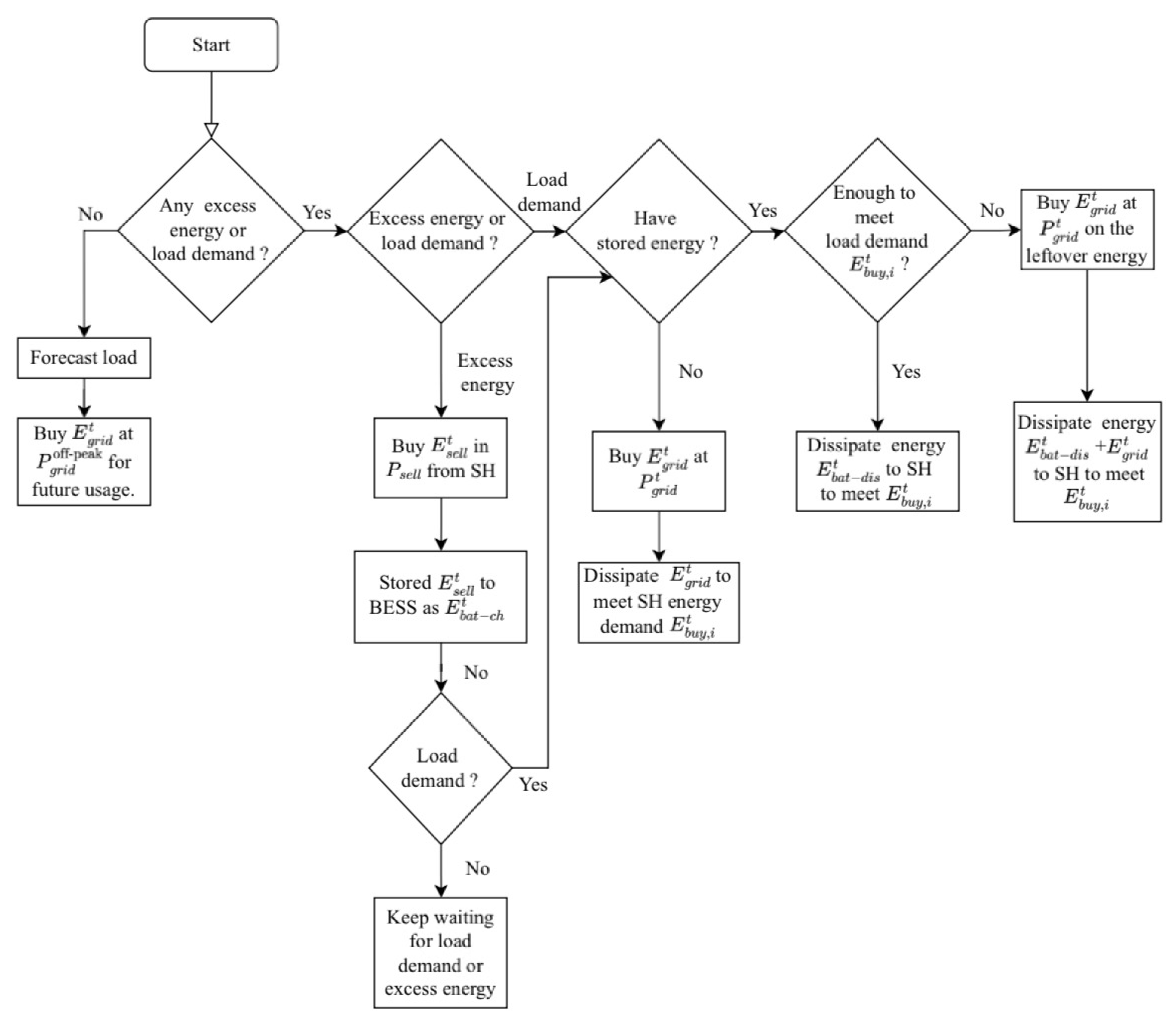
The AGG serves as the central energy coordinator, responsible for monitoring, managing, and optimizing energy flows within the community. By utilizing smart meters installed at each household, the AGG continuously collects data on power demand, PV generation, and electricity purchases from the grid. The AGG owns and operates the shared BESS, which stores excess solar energy generated by smart homes during the day and supplies it during the night or when local generation is insufficient. In addition, the AGG may purchase electricity from the grid during off-peak hours to store in the BESS and discharge during peak demand periods. This strategy supports a budget-balanced operation, meaning the AGG recovers its costs without seeking profit, while also helping to reduce electricity expenses for participating households. The operational flowchart of the AGG is illustrated in Figure 2.

3.2.2. Smart Homes

Each smart home is equipped with a rooftop PV system and a smart meter connected to the community’s energy trading platform. The primary function of the PV system is to meet the household’s own energy demand. When generation exceeds consumption, the surplus energy is automatically sold to the AGG at a fixed buyback rate ($p_{sell}$). All energy flows and financial transactions are recorded by the smart meter and integrated into the SEAMS. Prosumers benefit from a net billing mechanism, in which the energy they export is offset against their future consumption. In many cases, this results in a significant reduction in the electricity bill. In rare situations, the total cost may become negative, indicating net revenue. Conversely, when a home requires more energy than it generates, it purchases the additional energy from the AGG at a rate ($p_{buy}$) that is lower than the grid price ($p_{grid}^t$).

3.3. Pricing and Regulatory Constraints

In this model, energy pricing is centrally managed by the AGG. A fixed rate $p_{sell}$ is used to purchase surplus PV energy from prosumers, while a separate fixed rate $p_{buy}$ is applied when selling energy to households. The AGG operates under a budget-balanced pricing policy, ensuring that its total revenue from energy sales equals its total expenditure. This includes the cost of purchasing electricity from the grid and prosumers, battery degradation, and investment in the shared BESS.

Importantly, the selling price $p_{buy}$ is intentionally set as a fixed value determined by the SEAMS model, rather than being dynamically optimized. This approach prioritizes user simplicity and is intended to build understanding and trust among community members, many of whom may be unfamiliar with complex pricing mechanisms. A fixed rate also simplifies billing and communication within the community while still enabling meaningful cost savings through optimal energy scheduling and battery utilization.

Moreover, the model is designed to comply with Thailand’s regulatory constraint that prohibits residential grid export. As a result, all energy transactions must take place within the community. The AGG is allowed to purchase electricity from the grid but cannot sell any excess back to it, highlighting the need for effective local energy trading and storage.

4. Optimization Model (SEAMS)

In this section, we introduce the proposed optimization model for SEAMS. It is designed to manage a smart community energy trading scheme that coordinates energy flows between prosumer households, a centralized AGG, BESS, and the main electricity grid. The model’s objective is to minimize the total electricity cost for all households while maintaining financial neutrality for the AGG. The optimization model is formulated as an MILP. The model formulation incorporates key components such as energy trading, PV investment cost allocation, battery degradation, and TOU electricity pricing. It includes constraints to ensure energy balance, enforce battery operational logic, control pricing limits, and model household-level PV generation and demand. SEAMS enables cost-efficient coordination of distributed energy resources and supports scalable deployment of decentralized solar systems, particularly in the context of smart communities in Thailand.

4.1. Objective Function

For SEAMS, the objective function aims to minimize the total net electricity cost of all smart homes in the community through net billing, calculated as the total payment for electricity purchased from the AGG ($p_{buy}·E_{buy,i}^t$) minus the total revenue from selling surplus energy back to the AGG ($p_{sell}·E_{sell,i}^t$), plus the investment cost of all the residential PV systems ($C_{PV}^{inv}$). The objective function can be expressed as in Equation (1) below:

$$min\sum _{t=1}^T\sum _{i=1}^N\left(p_{buy}·E_{buy,i}^t-p_{sell}·E_{sell,i}^t\right)+C_{PV}^{inv}$$

(1)

where $p_{buy}$ is the electricity price paid by smart homes to the AGG (THB/kWh), and $p_{sell}$ is the fixed price for purchasing surplus energy from smart homes (THB/kWh). The variable $E_{buy,i}^t$ denotes the energy purchased by smart home i from the AGG at time t (kWh), while $E_{sell,i}^t$ represents the energy sold by smart home i to the AGG at time t (kWh). The term $C_{PV}^{inv}$ refers to the PV investment cost for all smart homes over the time horizon (THB). Lastly, N is the total number of smart homes, and T is the total number of time periods.

The objective function is summed across all houses and time periods, with variations in either the number of houses or the time period resulting in different outcomes. Additionally, it incorporates the investment cost of residential PV systems. Consequently, residents are responsible for these investment costs in exchange for the associated benefits.

PV Investment Cost

The PV investment cost varied depending on the time horizon and can be described as in Equation (2) below:

$$C_{PV}^{inv}=\sum _{i=1}^N{\displaystyle \frac{c_{PV}^{unit}\times P{V}_{size,i}}{L_{PV}}}$$

(2)

where $c_{PV}^{unit}$ is the investment cost per kW of PV capacity (THB/kW), $P{V}_{size,i}$ is the PV size installed at smart home i (kW), and $L_{PV}$ represents the lifetime of the PV system.

Therefore, if the simulation is run daily, the $C_{PV}^{inv}$ will change from the total PV investment to daily PV investment ($C_{PV,daily}^{inv}$). The amount of $C_{PV}^{inv}$ will depend on the lifetime of PV ($L_{PV}$) as if the time horizon increases, the denominator will be smaller as the unit changes from day to week/month resulting in the total cost investment will be larger.

Lastly, $P{V}_{size,i}$ is the PV size that will have to be chosen, where i illustrates the number of houses. If the houses in the community increases, the investment cost also has to increase due to more installations. Therefore, from all these variables, the formula in Equation (2) illustrates the function and aims to calculate the daily PV investment cost of the PV over its lifetime.

4.2. Aggregator Constraints

The AGG is responsible for balancing the energy flows between prosumer households, BESS, and the electricity grid. To ensure operational feasibility and financial neutrality, the following constraints are imposed on the AGG behavior.

4.2.1. Budget Balance Constraint

Budget balance or financial neutrality is a very crucial factor in keeping the system running. This constraint aims to save AGG from going into debt by saving too much cost for the residents. This constraint ensures that the AGG maintains financial balance, meaning it does not make a profit or incur a loss. Equation (3) shows the constraint for the budget balance of the AGG.

$$\sum _{t=1}^T\sum _{i=1}^N{p}_{buy}·E_{buy,i}^t=\sum _{t=1}^T\left(p_{grid}^t·E_{grid}^t\right)+\sum _{t=1}^T\sum _{i=1}^N\left(p_{sell}·E_{sell,i}^t\right)+C_{batt}^{deg}+C_{BESS}^{inv}$$

(3)

where $p_{grid}^t$ is the grid electricity price (THB/kWh), $E_{grid}^t$ is the energy imported from the grid at time t (kWh), $C_{batt}^{deg}$ is the total battery degradation cost (THB), and $C_{BESS}^{inv}$ is the BESS investment cost over the time horizon (THB).

In this constraint, the total income received from smart homes through electricity sales ($p_{buy}·E_{buy,i}^t$) must be equal to the total expenditures in the AGG, which is the summation of purchasing grid electricity ($p_{grid}^t·E_{grid}^t$), purchasing surplus energy from smart homes ($p_{sell}·E_{sell,i}^t$), battery degradation cost ($C_{batt}^{deg}$), and battery investment cost ($C_{BESS}^{inv}$).

Battery Degradation Cost

Equation (4) below aims to calculate the total battery degradation cost based on the total charging and discharging energy throughout the operation period. The energy charged into BESS ($E_{bat-ch}^t$) and the energy discharged from BESS ($E_{bat-dis}^t$) are generated by MILP, where it is the total amount of battery energy charged/discharged. Therefore, this effect as more cycle results in more degradation.

$$C_{batt}^{deg}=\gamma ·\sum _{t=1}^T\left(E_{bat-ch}^t+E_{bat-dis}^t\right)$$

(4)

where $\gamma$ represents the battery degradation cost coefficient, measured in THB/kWh. The variable $E_{bat-ch}^t$ denotes the amount of energy charged into the shared battery at time t (kWh), while $E_{bat-dis}^t$ indicates the energy discharged from the shared battery at time t (kWh).

Battery Investment Cost

BESS is a key element within SEAMS, making it essential for AGG to accurately estimate the investment cost of the community shared battery. Equation (5) below shows the battery investment cost, which aims to calculate the investment cost of the battery over its lifetime.

$$C_{BESS}^{inv}={\displaystyle \frac{c_{BESS}^{unit}\times BESS}{L_{BESS}}}$$

(5)

where $c_{BESS}^{unit}$ represents the investment cost per kWh of the BESS, expressed in THB/kWh. The parameter $L_{BESS}$ denotes the lifetime of the BESS.

Similarly to Equation (2), the BESS lifetime ($L_{BESS}$) depends on the time horizon chosen in a specific simulation, and the $BESS$ is the size of the battery chosen.

4.2.2. Price Limits

From the objective, SEAMS aims to lower the total cost as much as possible, especially from the grid electricity unit cost ($p_{grid}^t$). By that, the constraint in Equation (6) ensures that the optimized electricity unit cost that residents buy from AGG ($p_{buy}$) does not exceed the on-peak grid electricity unit cost ($p_{grid,on-peak}^t$). If the $p_{buy}$ exceeds $p_{grid,on-peak}^t$, then SEAMS is actually not beneficial and not practical.

$$p_{buy}\le p_{grid,on-peak}^t,\forall t$$

(6)

where $p_{grid,on-peak}^t$ is the on-peak electricity unit price of the Thailand grid (THB/kWh).

4.2.3. Energy Balance Constraint

Equation (7) below is readjusted from the power balancing equation from [29], where it ensures that, at each time period, the total incoming energy to the AGG equals the total outgoing energy. The energy balance constraint can be written as follows:

$$E_{grid}^t+E_{bat-dis}^t+\sum _{i=1}^N{E}_{sell,i}^t=E_{bat-ch}^t+\sum _{i=1}^N{E}_{buy,i}^t,\forall t$$

(7)

where $E_{grid}^t$ is the energy imported from the grid (kWh). After serving the SH demand, any surplus energy is stored in the shared BESS within its capacity and power limits. This constraint is very crucial as if the energy is not balanced, then the community will experience overgeneration or blackout at some period, which is not a preferred case. Furthermore, it can be seen that $E_{grid}^t+E_{bat-dis}^t+{\sum }_{i=1}^N{E}_{sell,i}^t$ is the incoming energy while $E_{bat-ch}^t+{\sum }_{i=1}^N{E}_{buy,i}^t$ is the outgoing energy of SEAMS.

4.2.4. Shared Battery Storage State of Charge (SOC) Update

Equation (8) below is used to update the battery SOC based on charging and discharging activities and governs the evolution of the battery’s state of charge (SOC) over time to ensure energy continuity across hourly intervals. This constraint updates the battery’s SOC at each time step t is based on the energy charged into and discharged from the battery during the previous interval, and can be written as follows:

$$SO{C}^t=SO{C}^{t-1}+{\displaystyle \frac{{\eta }_{ch}·E_{bat-ch}^t}{BESS}}-{\displaystyle \frac{E_{bat-dis}^t}{{\eta }_{dis}·BESS}},\forall t.$$

(8)

The SOC is normalized (on a 0–1 scale) by dividing the energy terms by the total battery capacity BESS. Charging efficiency ${\eta }_{ch}$ and discharging efficiency ${\eta }_{dis}$ are included to reflect real-world energy losses during storage operations. The variable $E_{bat-ch}^t$ and $E_{bat-dis}^t$ represent the energy charged and discharged at time t, respectively, while $SO{C}^t$ and $SO{C}^{t-1}$ is the state of charge at time t and $t-1$, respectively.

4.2.5. Battery SOC Cycle Constraint

To fully utilize the BESS, the battery SOC should return to the initial state at the end of the day. Basically, BESS energy should be prioritized to be used first until it runs out at the end of the day, and then restarted on the new day. By that, the constraint in Equation (9) ensures that the battery returns to its initial state of charge at the end of the day, and the battery starts each day from the same condition for consistent daily optimization while helping maintain daily energy neutrality for fair long-term operation. The constraint is written as follows:

$$SO{C}_{\mathrm{init}}=SO{C}_{\mathrm{end}}$$

(9)

where $SO{C}_{\mathrm{init}}$ is the initial state of charge of the shared battery, and $SO{C}_{\mathrm{end}}$ is the final state of charge of the shared battery at the end of the day.

4.2.6. Battery SOC Limits

The SOC of the battery must be maintained within predefined safe operating boundaries to prevent overcharging or deep discharging.

$$SO{C}_{min}\le SO{C}^t\le SO{C}_{max},\forall t$$

(10)

where $SO{C}_{min}$ denotes the minimum allowable state of charge (SOC) limit, and $SO{C}_{max}$ represents the maximum SOC limit.

4.2.7. Battery Power Limits

The battery power limit constraints ensure that the charging and discharging power of the shared battery remains within its rated capabilities at every time step. The constraints can be written as in Equations (11) and (12) below:

$$0\le P_{bat-ch}^t\le P_{bat-ch}^{max},\forall t$$

(11)

$$0\le P_{bat-ch}^t\le P_{bat-dis}^{max},\forall t$$

(12)

where $P_{bat-ch}^t$ and $P_{bat-dis}^t$ represent the battery’s charging and discharging power at hour t in kW, while $P_{bat-ch}^{max}$ and $P_{bat-dis}^{max}$ denote the maximum allowable charging and discharging rates in kW, respectively. These constraints are critical for ensuring the model respects the technical limitations of the inverter and battery hardware, preventing infeasible operation and supporting realistic simulation of energy dispatch in the SEAMS system.

4.2.8. Battery Operating Constraint

In BESS, charging and discharging energy simultaneously are impossible. By that, this constraint prevents the simultaneous charging and discharging of the shared battery. Moreover, this constraint also shapes the simulation to be MILP as it introduces the integer variable $x_{bat}^t$ in Equation (15). From that, when $x_{bat}^t$ = 1, the battery is allowed to charge and discharging is forced to zero. But when $x_{bat}^t$ = 0, the battery discharges and charging is disabled as in Equations (13) and (14). This constraint reflects the physical limitations of most battery systems and ensures realistic operation within the SEAMS framework. It also allows the optimizer to dynamically switch between charging and discharging modes based on cost efficiency and system needs. These constraints are written as follows:

$$E_{bat-ch}^t=x_{bat}^t\times P_{bat-ch}^t\times \Delta t,\forall t$$

(13)

$$E_{bat-dis}^t=(1-x_{bat}^t)\times P_{bat-dis}^t\times \Delta t,\forall t$$

(14)

$$x_{bat}^t=\left\{\begin{array}{cc}1,\hfill & \mathrm{if}\mathrm{charging}\mathrm{at}\mathrm{time}t\hfill \\ 0,\hfill & \mathrm{if}\mathrm{discharging}\mathrm{at}\mathrm{time}t\hfill \end{array}\right.\forall t$$

(15)

where $x_{bat}^t$ is the binary variable indicating the battery operation status at time t (1 if charging, 0 if discharging) and $\Delta t$ is the duration of each time.

4.3. Smart Home (SH) Constraints

SH inside SEAMS also plays a significant role inside the framework as they are the sources of PV generation of the community, sellers, and also the users. Therefore, SH needed constraints to make the MILP logic practical and accurate.

4.3.1. Energy Balance Constraint of SH

The energy balance constraint for each smart home (SH) ensures that household electricity demand is fully satisfied at every time step through available energy sources. This constraint is written as in Equation (16) below.

$$E_{load,i}^t=E_{PV-sel f,i}^t+E_{buy,i}^t,\forall i,t$$

(16)

where $E_{load,i}^t$ is the load demand of smart home i in kWh, $E_{PV-sel f,i}^t$ is the PV self-consumption in kWh, and $E_{buy,i}^t$ is the energy purchased from the AGG in kWh. $E_{load,i}^t$ represents the total energy demand of household i at hour t, which must be met either by self-consumed PV energy ($E_{PV-sel f,i}^t$) or by electricity purchased from the AGG ($E_{buy,i}^t$). This constraint ensures no household experiences an energy deficit and that all consumption is accounted for through local generation or AGG supply.

4.3.2. PV Generation Allocation Constraint

As SH can generate solar PV, they can actually use it to meet their load or sell it to AGG. Solar generation of SH $E_{PV,i}^t$ has to be greater than or equal to the self-use energy $E_{PV-Sel f,i}^t$ and energy sold to AGG $E_{sell,i}^t$ sum up as described in Equation (17) below. The equation can be expressed as follows:

$$E_{PV,i}^t\ge E_{PV-sel f,i}^t+E_{sell,i}^t,\forall i,t$$

(17)

where $E_{PV,i}^t$ is the total PV generation of smart home i in kWh. This constraint needs to exist because if there is no PV energy generated, then there should not be any available energy going out. Therefore, this constraint allocates PV generation between self-consumption and surplus sold to the AGG, without exceeding the available generation.

4.3.3. Non-Negativity Constraints

As energy variables cannot be negative practically, this constraint ensures all energy variables are non-negative.

$$E_{load,i}^t\ge 0,\forall i,t$$

(18)

$$E_{PV,i}^t\ge 0,\forall i,t$$

(19)

$$E_{PV-sel f,i}^t\ge 0,\forall i,t$$

(20)

$$E_{sell,i}^t\ge 0,\forall i,t$$

(21)

$$E_{buy,i}^t\ge 0,\forall i,t$$

(22)

5. Results and Discussion

This section presents the simulation results and analysis of the proposed SEAMS framework under conditions specific to Thailand. Various case scenarios are evaluated to examine the system’s performance in terms of energy balance, battery operation, electricity cost, and the optimal sizing of PV and battery systems. In addition, the impact of key parameters, such as PV capacity, battery size, and the level of prosumer participation, is analyzed to assess their influence on community-wide energy costs and system behavior.

5.1. Simulation Setup and Parameters

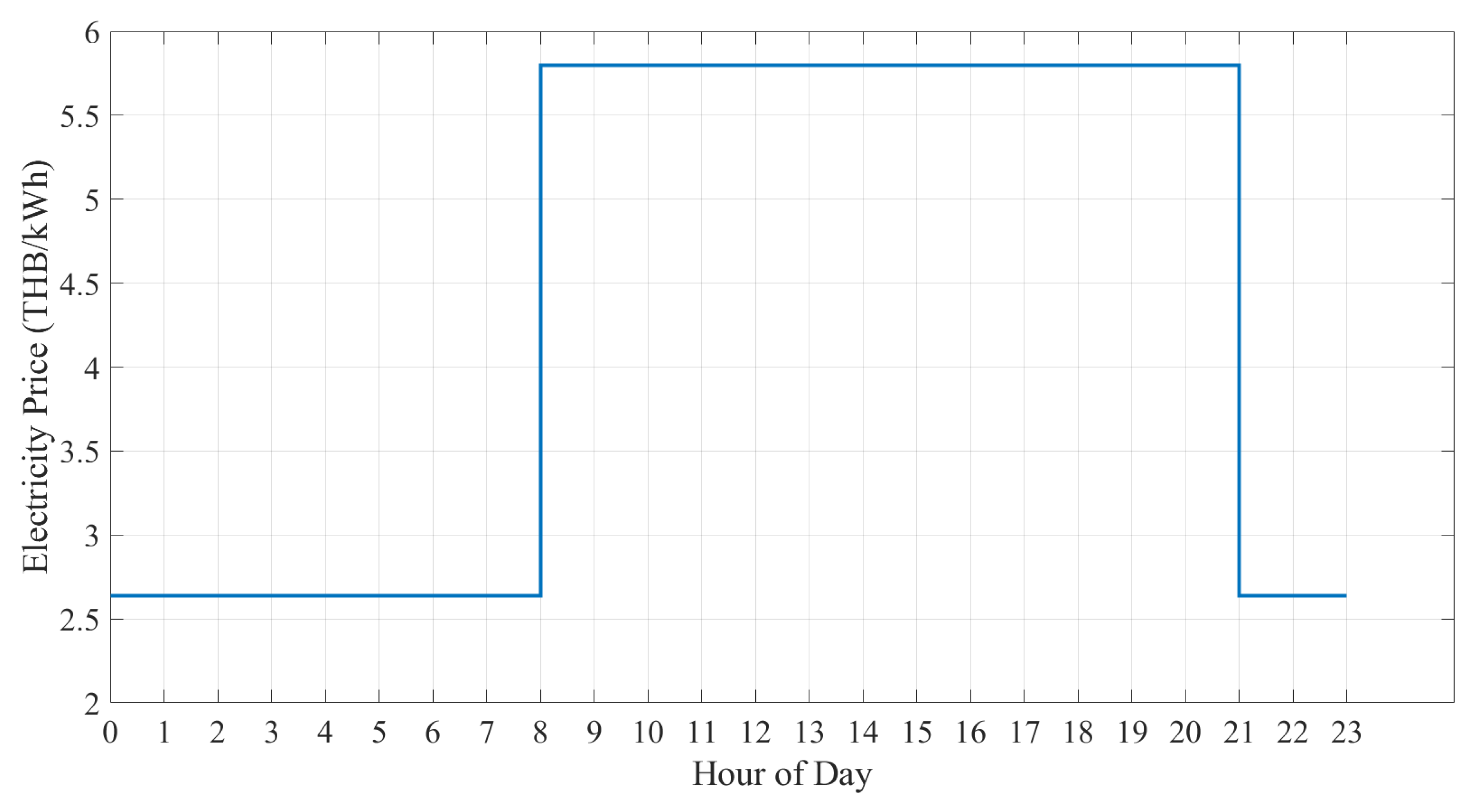
The SEAMS framework is validated using an MILP approach based on the mathematical formulation presented in Section 4. The TOU electricity pricing used in the simulation is derived from the official tariff structure published by the PEA of Thailand [56] as shown in Figure 3.

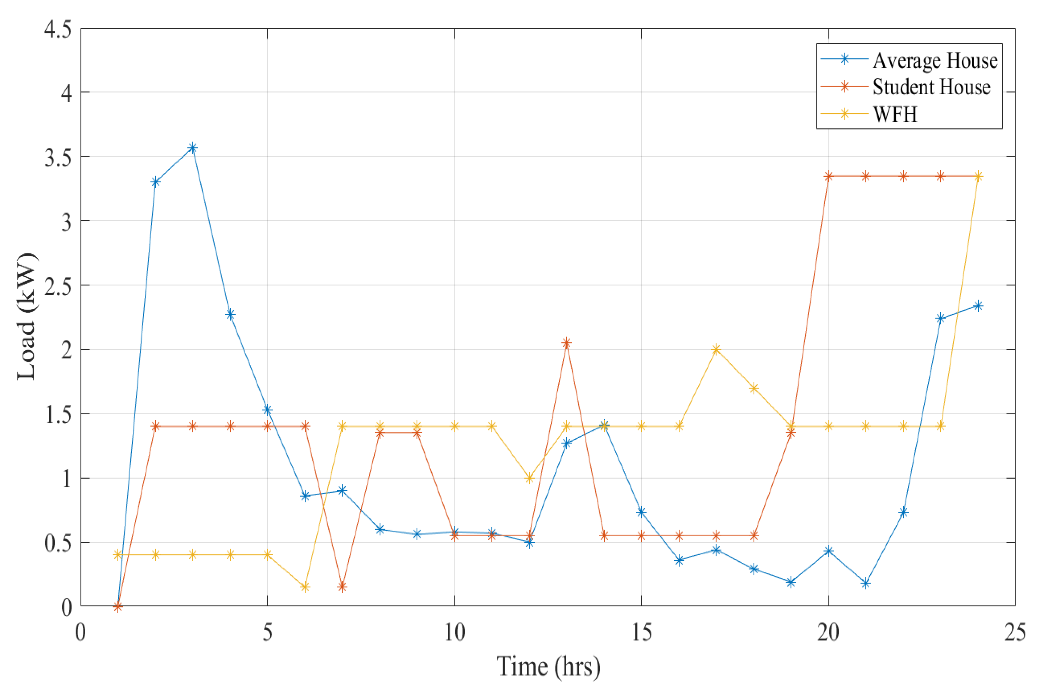
In this simulation, the SEAMS framework is applied to a community consisting of 10 smart homes (SHs), including both prosumers and consumers. The simulation considers three types of houses, each with a distinct load profile. Figure 4 illustrates the load profiles of the three house types: high-load houses (work-from-home households), medium-load houses (average households), and low-load houses (student households). The homes are classified into these categories as follows: houses 3, 6, and 9 are high-load; houses 1, 4, 7, and 10 are medium-load; and houses 2, 5, and 8 are low-load. The load data are based on [29,57], which focus on hot-climate countries and are suitable for modeling conditions in Thailand. Although the household load profiles are not sourced from a specific Thai community, they follow patterns commonly used in prior Thai-focused studies, offering reasonable representation for typical residential consumption in hot climates. PV investment costs are sourced from Thai market data provided by [58], while battery energy storage system (BESS) investment costs are based on [59]. Regarding system lifetimes, the BESS is assumed to have a lifespan of 10 years, based on [60], and the PV system is assumed to last 25 years, according to [61]. The battery degradation cost coefficient ($\gamma$) is calculated using the method from [62], considering a depth of discharge (DOD) of 80% from [63] and the total cycle life from [64]. These values are then used in Equation (4) to obtain the degradation cost. Finally, the battery state of charge (SOC) is constrained between 20% and 80%, with a round-trip efficiency of 90%, based on parameters from [29], which represent the standard battery state. While climate-specific degradation data for Thailand is limited, the selected parameters reflect conditions typical of hot-climate regions and are consistent with degradation models adopted in Thai simulation studies. Since degradation primarily depends on energy throughput and usage cycles, and most battery systems in Thailand are imported with similar specifications, the model remains applicable to the Thai context. Combined with localized PV generation profiles (from Rangsit, Pathum Thani), TOU tariff structures, and investment costs sourced from Thai markets, the simulation setup reflects the operational and regulatory context of smart communities in Thailand.

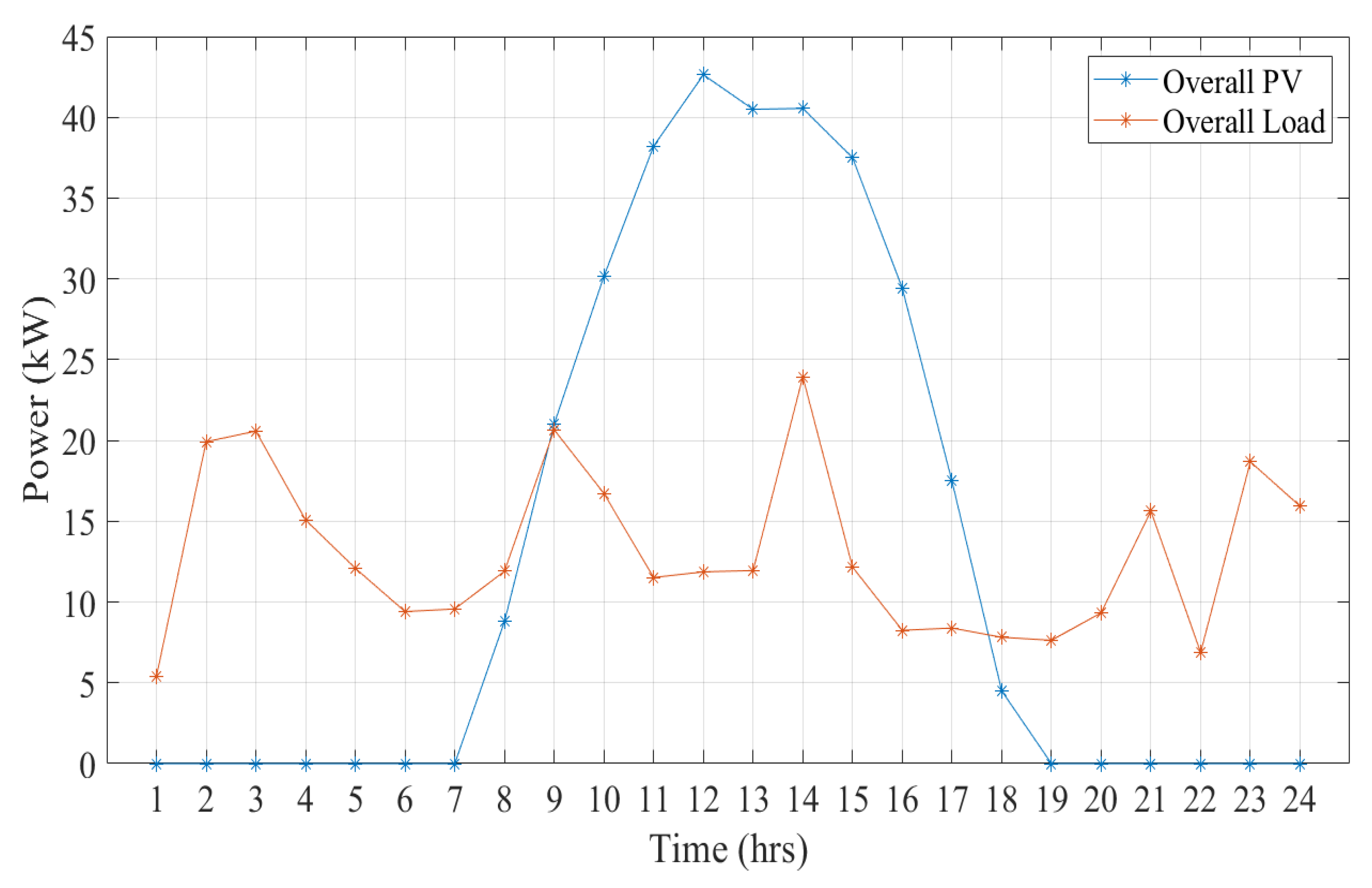
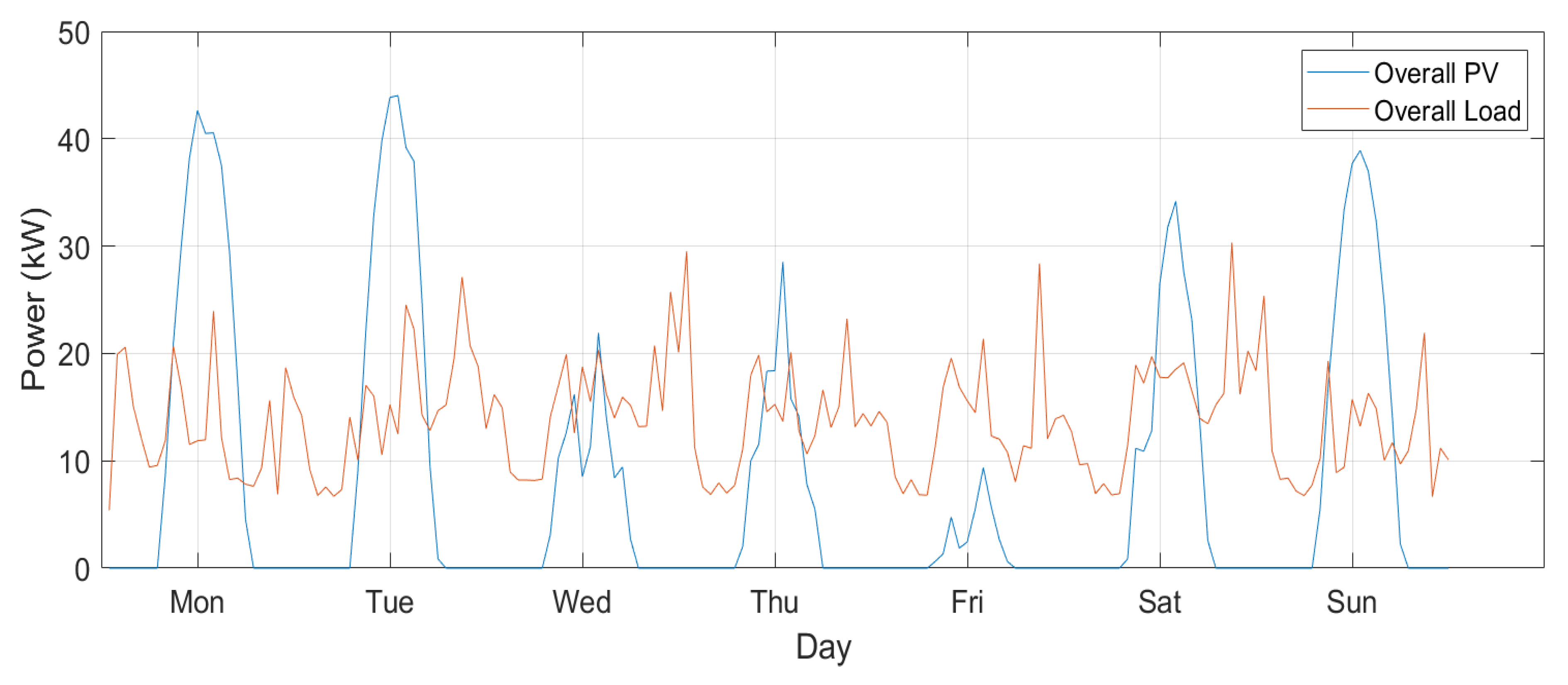
In Figure 5, PV generation in Thailand exhibits a typical diurnal pattern, beginning around 07:00, peaking between 11:00 and 13:00 at over 43 kW, and declining by 18:00. In contrast, the aggregated residential load profile shows demand peaks in the early morning and late evening, resulting in a temporal mismatch between energy generation and consumption. To address this issue, the system integrates a BESS. Consequently, determining the optimal battery size for a given community is critical for minimizing total electricity costs.

5.2. Daily System Behavior

This subsection analyzes the operational behavior of the SEAMS model under a fixed configuration to provide insights into energy flows and component interactions. Specifically, the shared battery capacity is set at 75 kWh, and each prosumer household is assumed to have a rooftop PV system with a capacity of 60 kW. The objective is to examine how energy is generated, stored, consumed, and exchanged within the community over the course of a typical day. Key system behaviors, including energy profiles, energy balance, battery state of charge (SOC), and charging and discharging patterns, are visualized and discussed.

Figure 6 illustrates the hourly energy profile of the solar community, showing power contributions from PV generation, household load, grid import, and battery charging and discharging. The PV and load curves follow the same characteristics described previously. To address the mismatch between PV generation and load demand, the system utilizes the BESS, which begins charging during the midday period (10:00 to 13:00). Charging occurs only during this time because the BESS capacity is limited. Once the BESS is fully charged, the remaining PV energy is consumed directly by the prosumers. After PV generation ends for the day, the BESS discharges to meet evening demand, particularly between 17:00 and 24:00. The discharge period is limited to this window because the stored energy is only sufficient to cover consumption until midnight. Beyond that point, the grid supplies the remaining energy demand. While this reliance on the grid may seem non-ideal, purchasing electricity during off-peak hours can be more cost-effective than investing in an oversized BESS capable of supplying energy throughout the entire night.

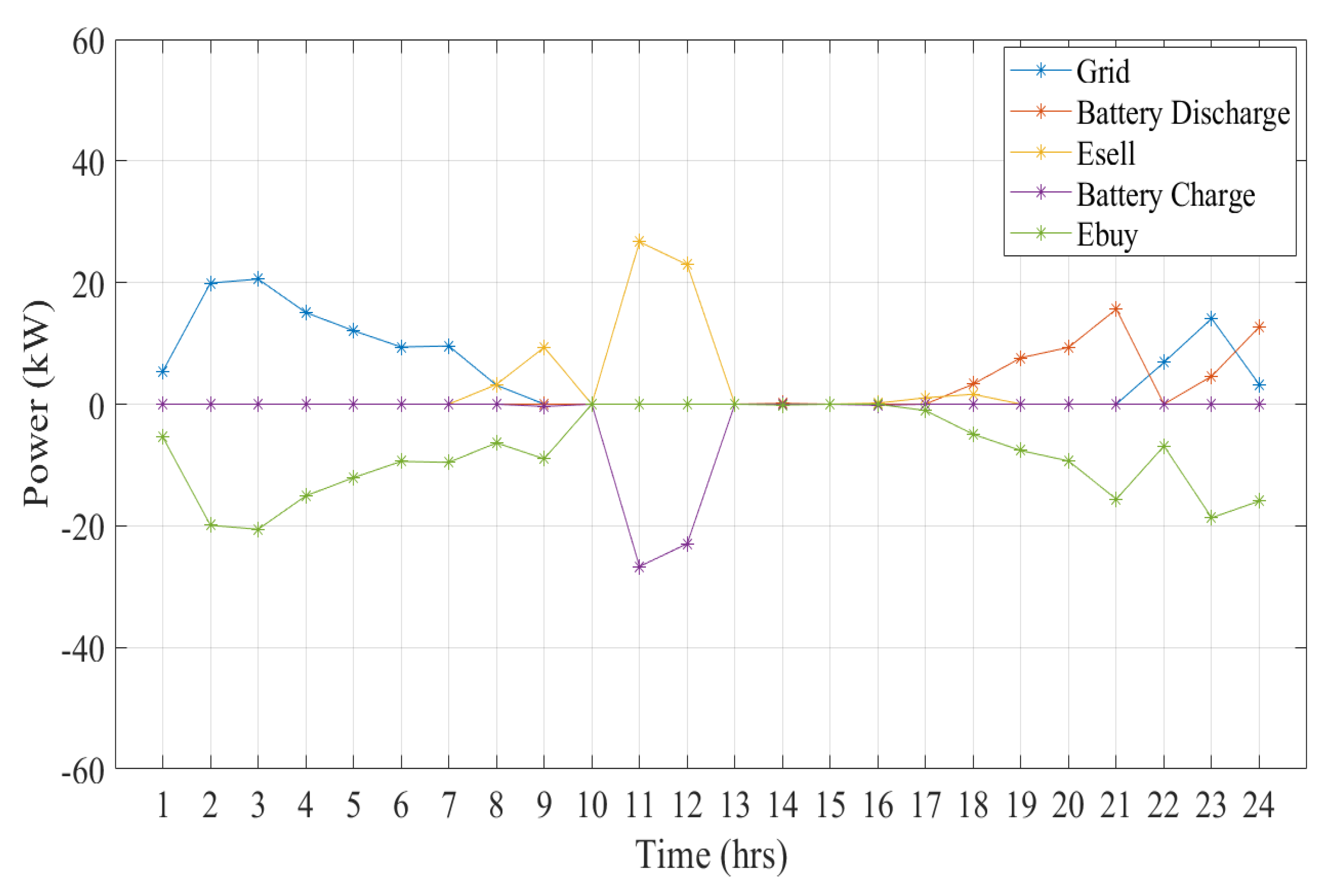
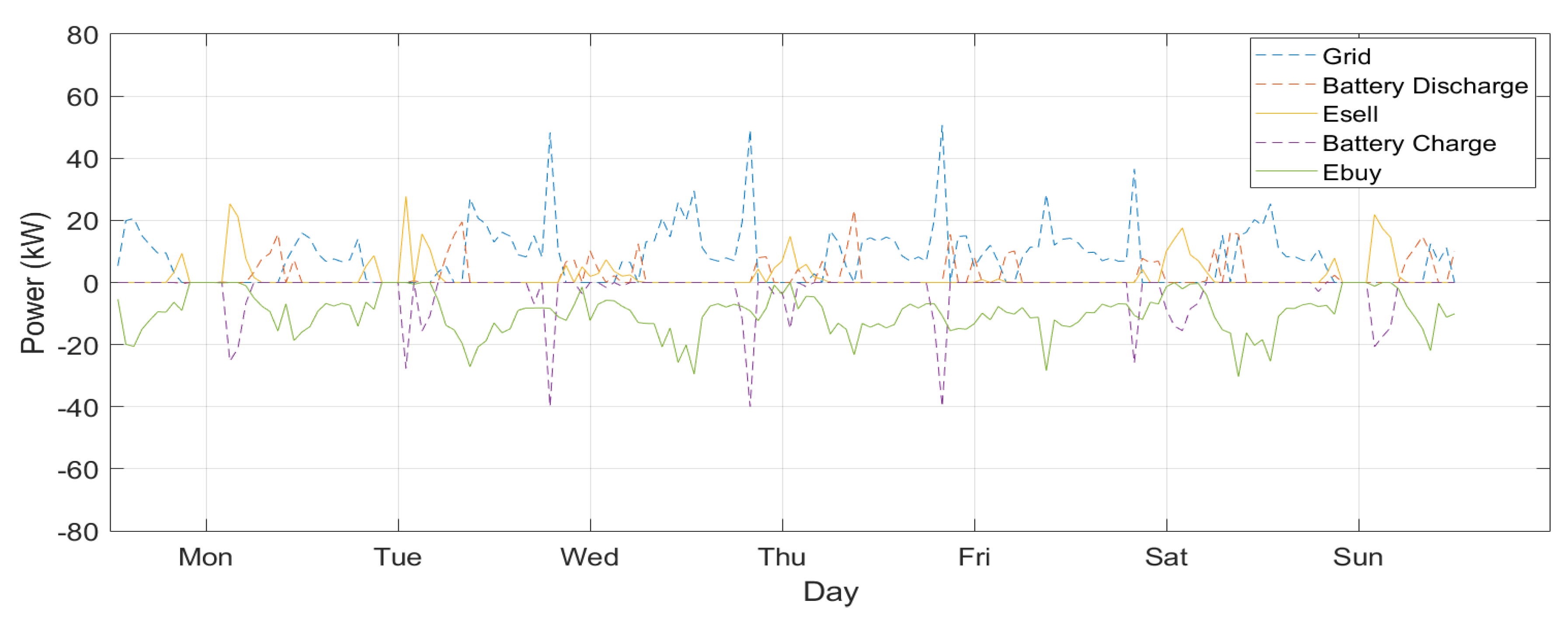
Furthermore, maintaining energy balance is a critical aspect of the SEAMS framework, as the total energy supply must always match the demand. Figure 7 illustrates the system’s energy balance over a 24 h period. This plot is used to verify that the sum of all energy inflows and outflows equals the total aggregated load demand at each time step. From the figure, it is evident that all sources and sinks, including grid import, battery charging and discharging, and energy trading between households and the AGG, are dynamically balanced, resulting in a symmetrical profile over the daily cycle. Together, Figure 6 and Figure 7 demonstrate that the BESS plays a central role in achieving efficient operation and maintaining energy balance within the proposed SEAMS framework.

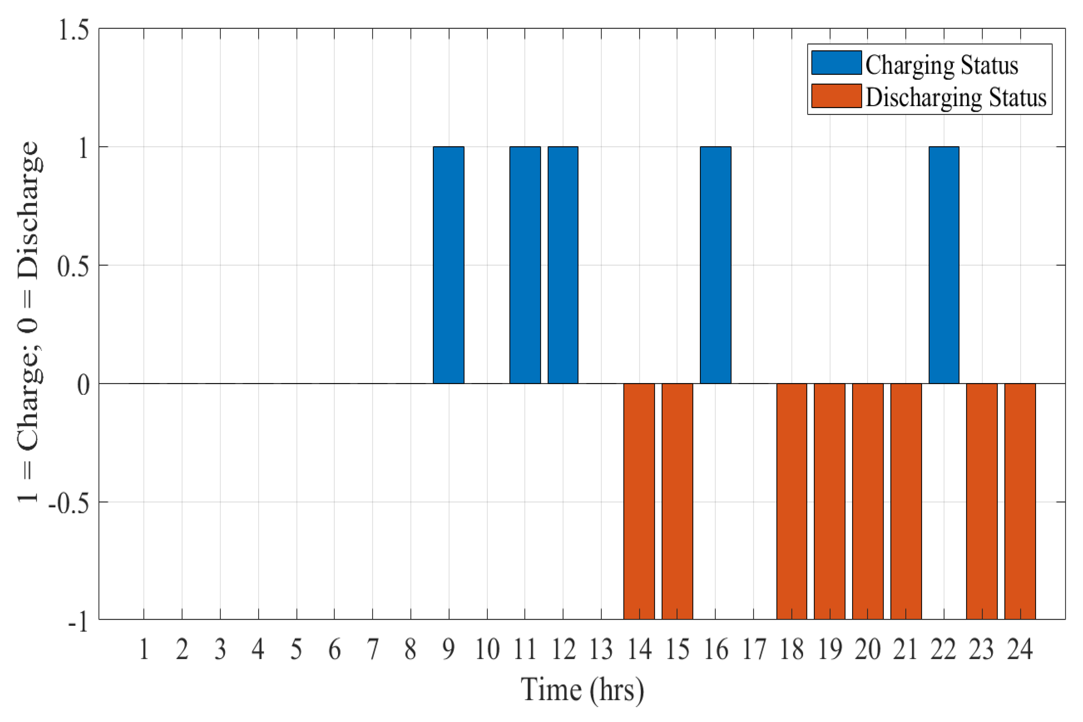
For the BESS, the SOC and charging status are critical indicators of operational behavior. Based on the simulation results, Figure 8 and Figure 9 illustrate the trends of both variables. For the binary charging state, the system enforces a mutually exclusive logic in which charging (represented by 1) and discharging (represented by 0) cannot occur at the same time. As shown, battery charging primarily occurs during solar peak hours, particularly between 11:00 and 13:00, with brief additional charging observed around 15:00 and 22:00. These periods align with surplus PV generation and energy intake by the AGG. Moreover, a discharging event can be observed between 14:00 and 15:00 in Figure 9. This occurs due to a small amount of energy being discharged during that hour, which is further confirmed by the energy balance shown in Figure 7 and the SOC profile in Figure 8. For the SOC profile, a rapid increase in SOC is observed starting at hour 12, rising from the minimum limit of 20 percent to the maximum of 80 percent by approximately hour 13. This increase corresponds to the charging phase, which is also visible in the energy profile in Figure 6. After reaching full charge, the SOC remains steady for several hours until discharging begins around 18:00, coinciding with the evening peak in household electricity demand. The battery continues discharging through the late evening, and the SOC gradually declines until it returns to 20 percent by midnight, completing the daily storage cycle.

5.3. Optimal Sizing of Battery and PV

Based on the MILP simulation using the equations defined in Section 4, the global optimization of BESS size is performed by varying the battery capacity from 0 kWh to 300 kWh across different PV system sizes to identify the configuration that yields the lowest total electricity cost. Figure 10 and Figure 11 present the resulting cost trends and clearly indicate the optimal sizes for both the BESS and PV systems.

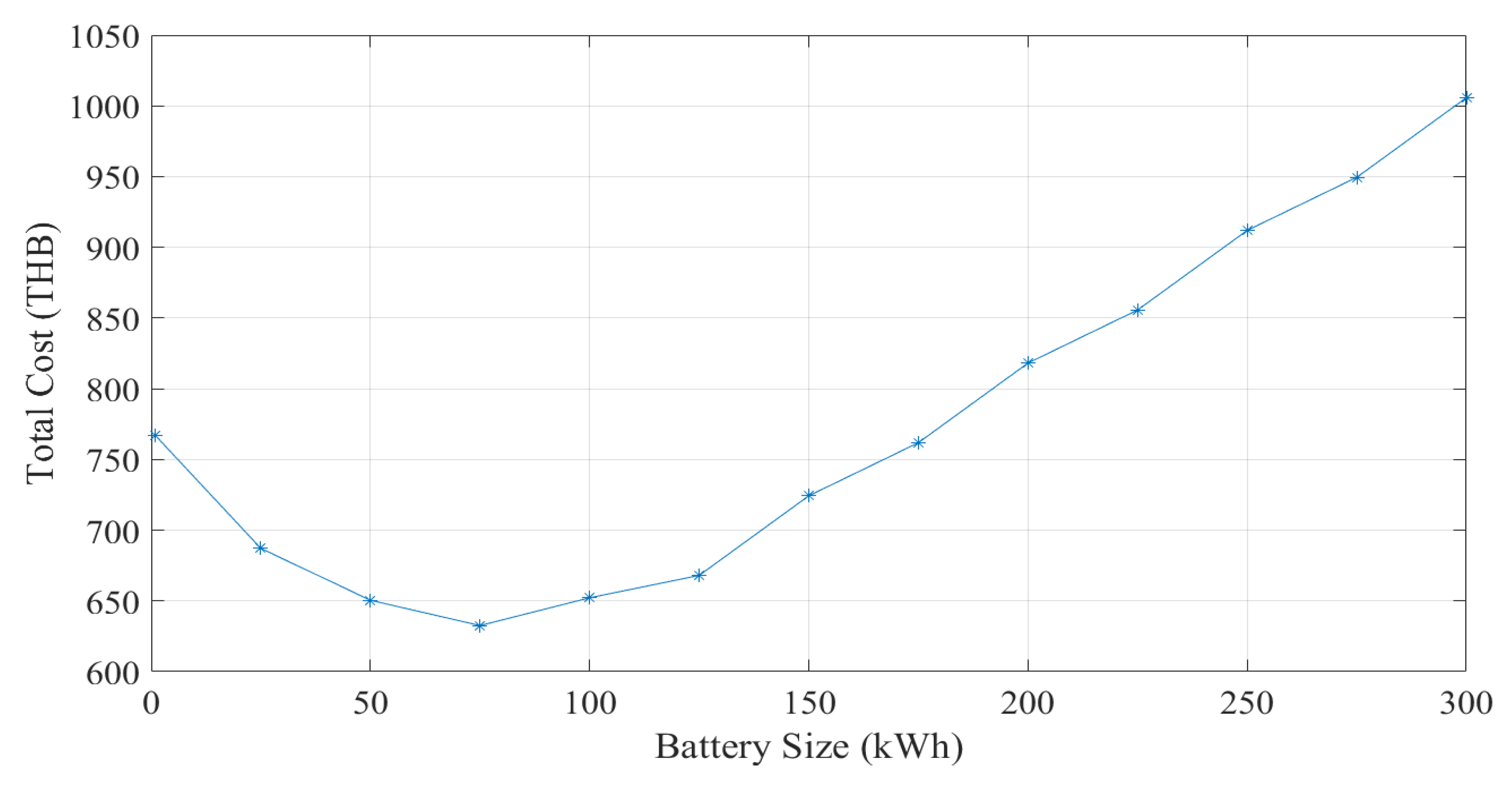
Focusing first on the BESS sizing results in Figure 10, the total cost curve exhibits an inverted bell shape. When the BESS size is too small (between 1 and 75 kWh), the total cost remains high due to increased reliance on grid electricity during peak pricing periods. On the other hand, when the BESS size exceeds 75 kWh, the marginal benefit from further cost savings becomes insufficient to offset the additional investment and degradation costs associated with a larger battery. Therefore, the optimal BESS size in this scenario is approximately 75 kWh. The results confirm the nonlinear nature of cost optimization in energy storage deployment, as illustrated in Figure 10. Oversizing the BESS leads to unnecessary capital expenditure, while undersizing results in missed opportunities to reduce costs through more effective solar energy utilization.

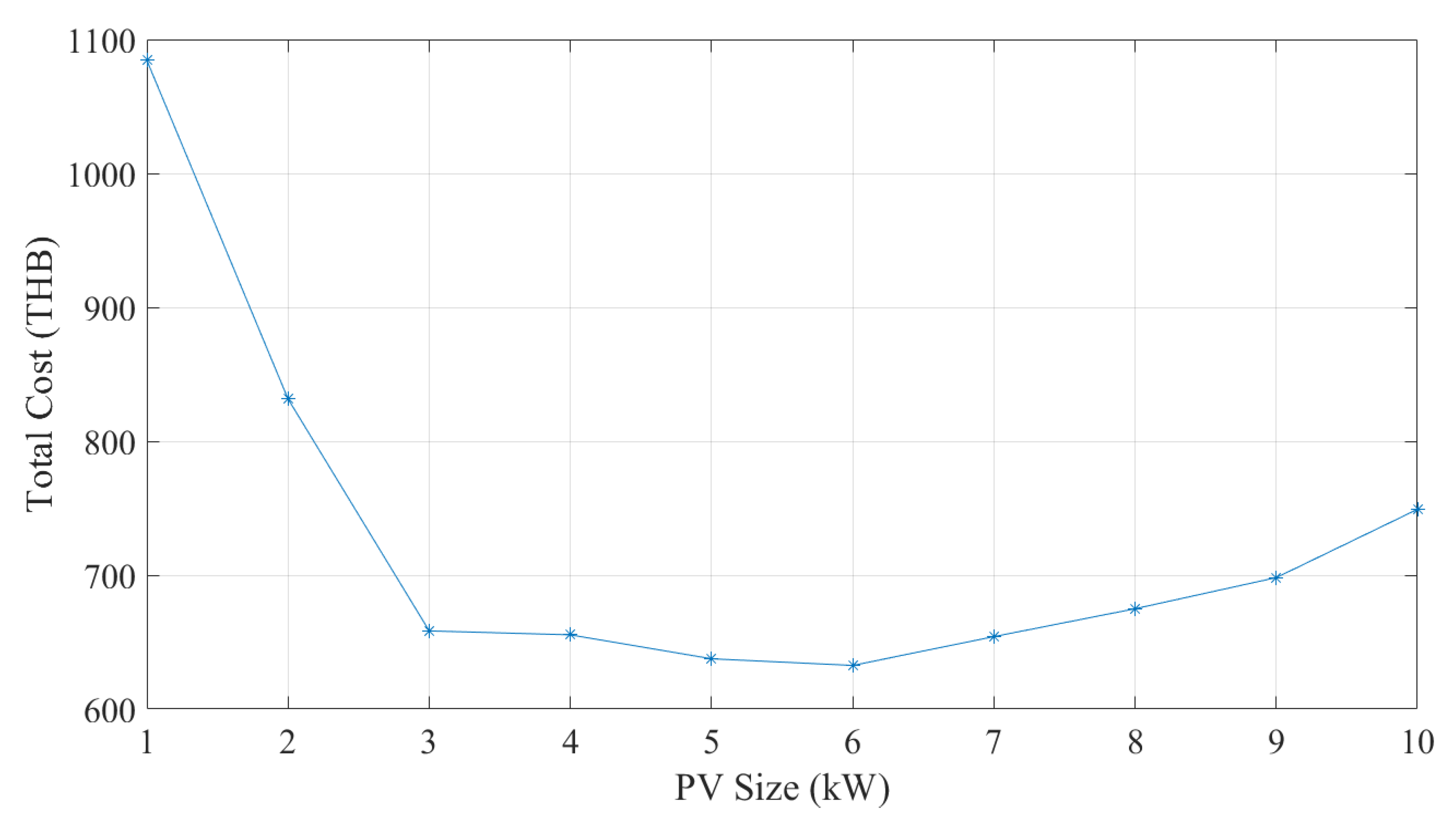
For PV system sizing, the global optimization results are presented in Figure 11. This figure shows the total cost of the solar community system as a function of installed PV capacity and is used to identify the optimal PV size for cost minimization. The results display a convex cost curve (inverted bell shape), indicating a well-defined economic optimum. Notably, the curve exhibits a similar trend to that observed in the BESS sizing analysis shown in Figure 10.

A key observation is the sharp decline in total cost as PV capacity increases from 1 kW to 3 kW per household. In this range, the system shifts from a heavy reliance on grid electricity to partial energy independence. At lower capacities (1–3 kW), PV output is insufficient to meet daytime load demand, resulting in significant grid imports. However, each additional kilowatt installed within this range displaces costly grid consumption with self-generated solar energy. Furthermore, the increased PV generation enhances BESS utilization by enabling more energy to be stored for use during evening hours, thereby amplifying the overall cost savings. Between 4 kW and 6 kW, the total cost continues to decrease, though at a slower rate. In this interval, PV generation begins to meet most of the community’s daytime demand, and surplus energy emerges. The BESS captures some of this excess, but its limited storage capacity restricts full utilization. As a result, the marginal benefit of further PV capacity additions diminishes, leading to a more gradual reduction in total cost. At 6 kW per household, the system reaches its minimum total cost, approximately 632.58 THB, representing the optimal balance between capital investment and operational savings. Beyond this point, additional PV capacity causes a slight increase in total cost due to overgeneration. The surplus energy cannot be fully consumed or economically stored, leading to underutilized capacity and inefficient capital deployment.

In summary, the results underscore the importance of right-sizing PV systems to achieve cost-optimal operation in community-based solar energy systems. Installing 6 kW of PV per household yields the lowest total cost by maximizing solar self-consumption, minimizing grid dependency, and avoiding excess investment in underutilized capacity. Additionally, the optimal PV size of 6 kW per household aligns well with Thailand’s high solar potential. For a community of just 10 households, this results in a total installed PV capacity of 60 kW, which is relatively large. This outcome reflects the country’s high solar irradiance levels, highlighting Thailand’s strong suitability for decentralized solar energy adoption. The findings affirm that Thailand is well-positioned to implement community-scale solar systems effectively.

To provide a three-dimensional perspective on the combined impact of PV size and BESS capacity on the total system cost, Figure 12 illustrates the results clearly. The surface reveals a distinct cost-minimization valley around PV sizes of 4 to 6 kW and battery capacities of 100 to 150 kWh, where the total cost reaches its lowest range, approximately 640 to 680 THB. However, the most optimal configuration remains at a PV size of 6 kW and a BESS capacity of 70 to 75 kWh. This region represents the most balanced setup, effectively utilizing available solar generation and storage while avoiding overinvestment. In terms of surface characteristics, the cost curve exhibits a U-shaped profile along both dimensions. When the BESS capacity exceeds 70 to 75 kWh, the total cost increases due to higher capital costs and diminishing returns from surplus storage capacity. Similarly, increasing PV size beyond 6 kW results in higher costs, primarily due to overgeneration that cannot be effectively stored or used, leading to underutilized investment. On the opposite end of the spectrum, under-sizing either the PV system or the BESS leads to increased dependency on grid electricity, thereby raising the total cost.

For sensitivity analysis, it was conducted to evaluate the impact of battery and photovoltaic (PV) system sizing on the total energy cost of the community energy-sharing model. Figure 10 illustrates the relationship between total cost and battery size, revealing a U-shaped trend. Specifically, increasing battery capacity initially reduces total cost due to enhanced self-consumption and reduced grid dependency, reaching an optimal cost point around 75 kWh. However, beyond this range, further capacity increments result in diminishing returns, as the marginal cost of additional storage outweighs energy cost savings. Similarly, Figure 11 shows the sensitivity of total cost to PV size. A sharp cost reduction is observed as PV size increases from 1 kW to around 5–6 kW. This range represents the optimal point where solar generation closely matches household demand and storage capacity, minimizing grid purchases. Conversely, over-sizing the PV system beyond this point leads to increased costs due to underutilized excess generation, especially in the absence of feed-in tariffs or grid export incentives.

To sum up, the total energy cost is highly sensitive to both battery and PV system sizes. Increasing battery capacity initially reduces cost due to improved solar energy utilization, but becomes counterproductive beyond 75 kWh, where additional storage yields diminishing economic returns. Similarly, increasing PV size significantly reduces cost up to around 5–6 kW, after which oversizing leads to underutilized generation and increased investment cost. The optimal configuration for minimizing total cost lies in a balanced combination of 6 kW PV and 75 kWh battery capacity. Deviating from this balance either by under-sizing or over-sizing results, in higher overall system costs.

5.4. Weekly System Behavior

To complement the daily simulation results, a full one-week simulation was conducted to capture the broader temporal dynamics of the SEAMS framework. Unlike single-day analysis, the week-long evaluation reveals how the system responds to naturally occurring variability in solar irradiance and residential load patterns. This timeframe better reflects real-world operational challenges such as partial cloud cover, inconsistent household activity, and battery cycling trends. The PV generation profile for the week was obtained using PVWatts, which already incorporates weather variability specific to the location of Pathum Thani, Thailand. As shown in Figure 13, the PV output varies significantly across days, illustrating real-world solar variability, including the effects of cloud cover and reduced generation consistent with monsoon season conditions.

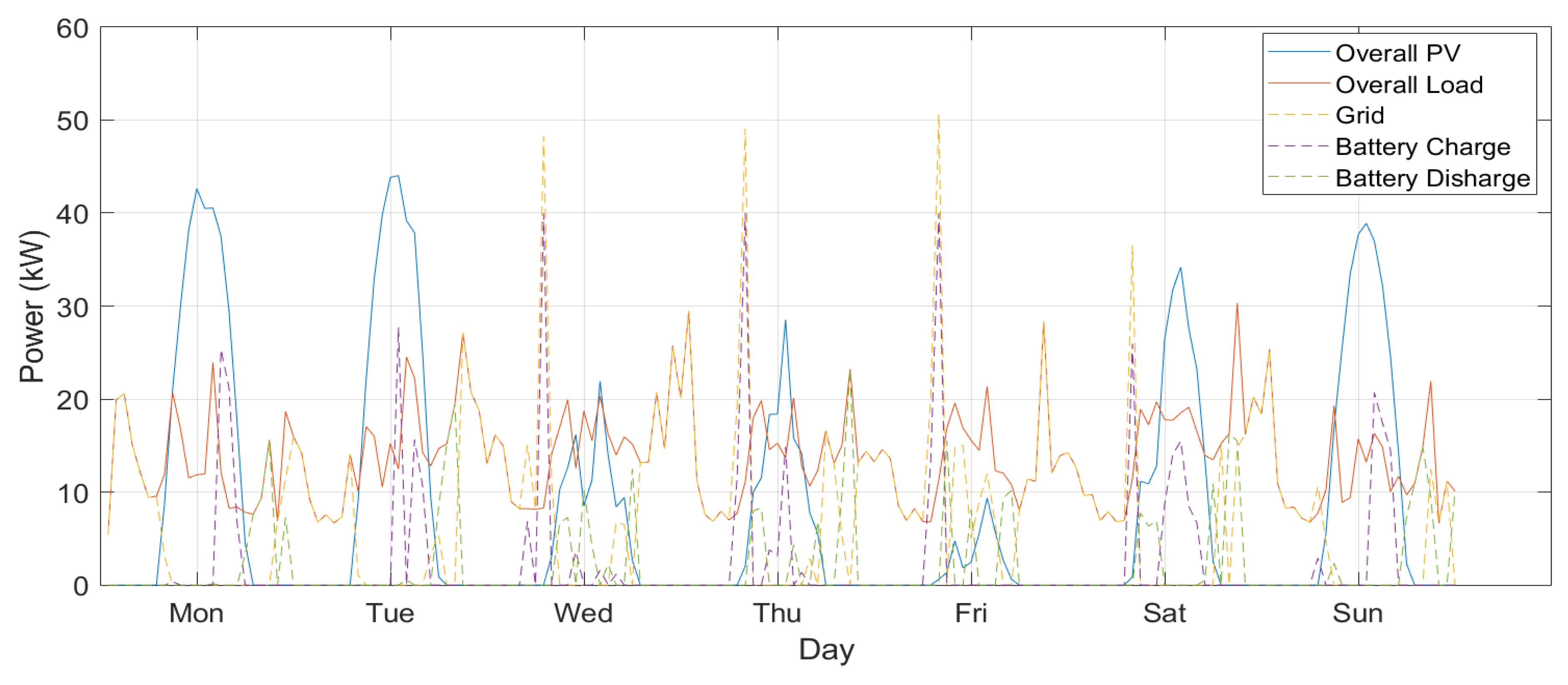
The weekly simulation results reveal the intricate interplay between fluctuating solar generation, variable household demand, and the operational limits of the energy storage system in the community. As shown in Figure 13, PV generation follows a consistent diurnal pattern but exhibits significant variation in daily yield due to weather conditions. For example, on Monday, a clear day, the PV system reached a peak output of around 43 kW. In contrast, on Friday, which experienced heavy cloud cover, the peak dropped to only 9 kW. This represents up to 79% reduction caused by decreased solar irradiance.

Meanwhile, household load profiles fluctuate throughout the week. Some days, such as Wednesday, exhibit elevated consumption due to evening peak activity, while others show lower overall demand. However, even on days with lower consumption, such as Thursday or Sunday, the timing mismatch between PV availability (midday) and load peaks (morning and evening) results in either curtailed solar energy or increased reliance on the grid. Since PV cannot fully meet real-time demand, this leads to higher total costs and elevated $p_{buy}$, due to the need to purchase electricity from the grid at higher prices.

As seen in Figure 14, grid imports increase during periods of low PV generation or high household load. Battery dynamics in Figure 15 illustrate efforts to mitigate this mismatch by charging during midday and discharging in the evening. However, battery capacity and timing constraints prevent a full offset of the load. This is especially evident on days like Friday, when low solar yield results in simultaneous grid import and battery discharge, reflecting a systemic energy deficiency leading to higher total costs for residents. To compare, this can be seen in daily cases that the PV system can cover most of the load, preventing the Agg from buying energy from the grid, and also maximizing the utilization of the battery, making the net total cost of the community lower and more optimal.

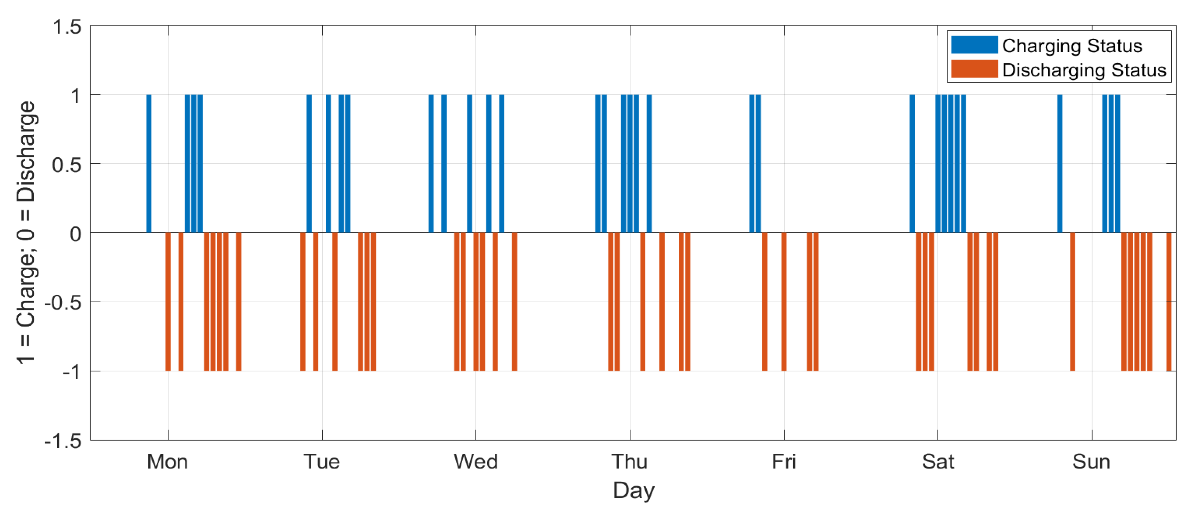
For the weekly SOC and charging status, Figure 16 and Figure 17 illustrate the battery’s charging and discharging behavior over a one-week period in the solar-powered Thai community. As shown in Figure 14, the charging and discharging power vary significantly throughout the week. This variation is strongly influenced by both the intermittent nature of solar irradiance, which is affected by weather conditions such as sunny, cloudy, or rainy days, and the fluctuating community load demand. On clear days with high solar irradiance, the battery exhibits intensive charging during midday when PV generation exceeds load demand. In contrast, on overcast or rainy days, such as Wednesday or Friday, the available PV energy is insufficient. As a result, the battery charges very little compared to other days, indicating underutilization. This leads to heavier reliance on battery discharge and grid imports to meet peak evening demand, contributing to higher electricity costs. These behavioral patterns are further confirmed in Figure 17, where the binary battery operation status shows distinct charging and discharging intervals for each day. This indicates the system’s dynamic responsiveness to real-time conditions. The battery charges when excess PV is available and discharges when demand exceeds immediate supply. Moreover, this cycling behavior directly affects battery degradation cost, which is considered in the model through total energy throughput. Higher cycling frequency or deeper discharges on days with poor solar input lead to increased battery wear, contributing to long-term operational costs.

5.5. Comparison of Different Simulation Horizons

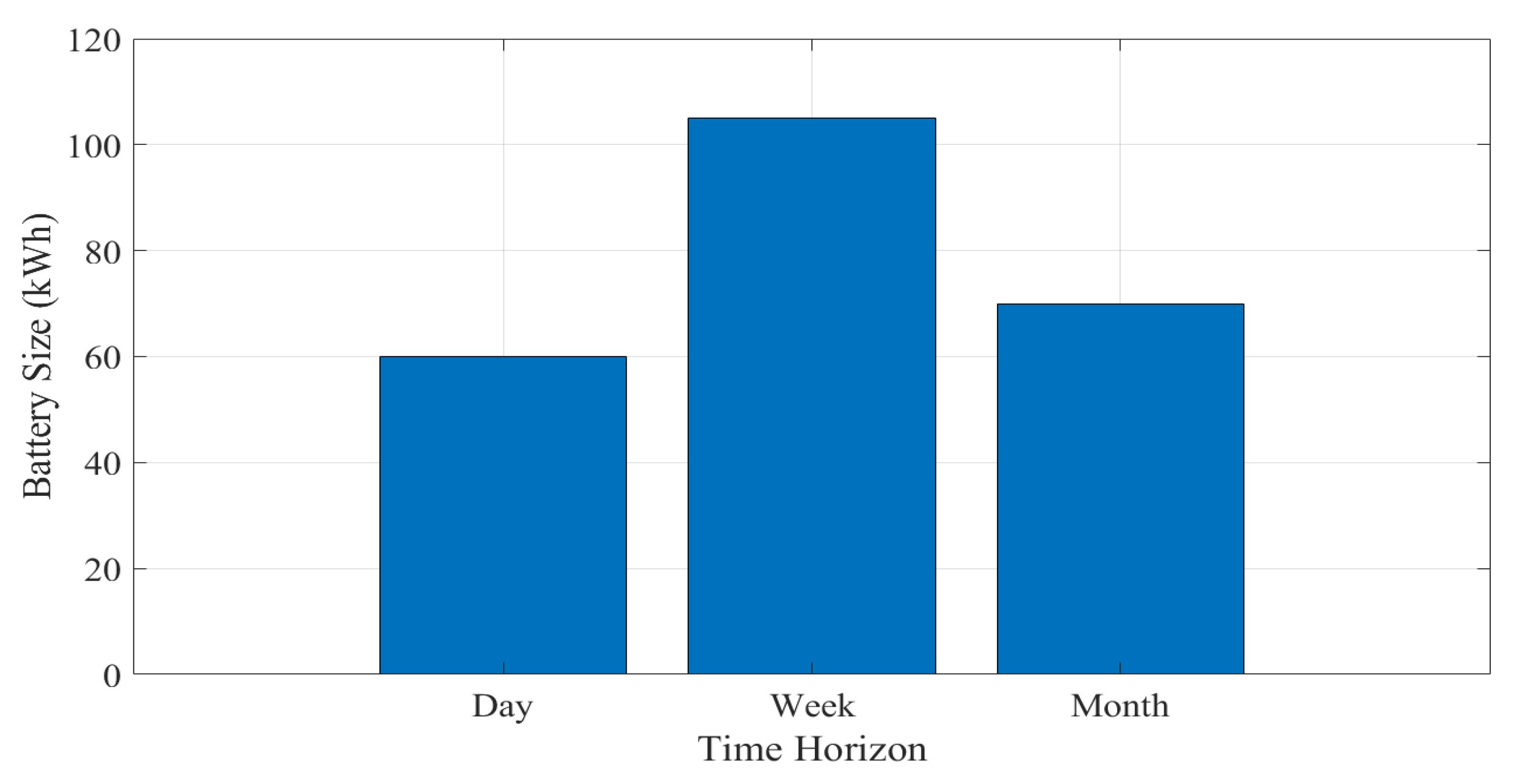
Overall, Figure 18 and Figure 19 illustrate the optimal BESS and PV sizes across different time horizons, including daily, weekly, and monthly simulations. For the weekly and monthly horizons, PV generation is subject to fluctuations due to intermittency, and the load profile also varies from day to day. As a result, the MILP-based optimization produces different outcomes depending on the selected time horizon. However, it can be observed that the daily and monthly results for both optimal BESS and PV sizes are relatively consistent. The only result that deviates significantly is from the weekly simulation. After multiple simulations and detailed analysis, it was found that the weekly time horizon is too short for the optimizer to effectively adapt to the variability in PV generation and load. Therefore, weekly optimization is less reliable and is better suited for understanding fluctuation patterns rather than determining precise system sizing. In contrast, monthly simulations also capture fluctuations in load and PV generation, but the longer time period (30 days) allows the optimizer to adjust and achieve more accurate results, where it reduces down to be closer to the daily, yielding more accurate results. Based on these findings, it can be concluded that the optimal BESS size falls between 70 and 75 kWh, and the optimal PV size is 6 kW per household.

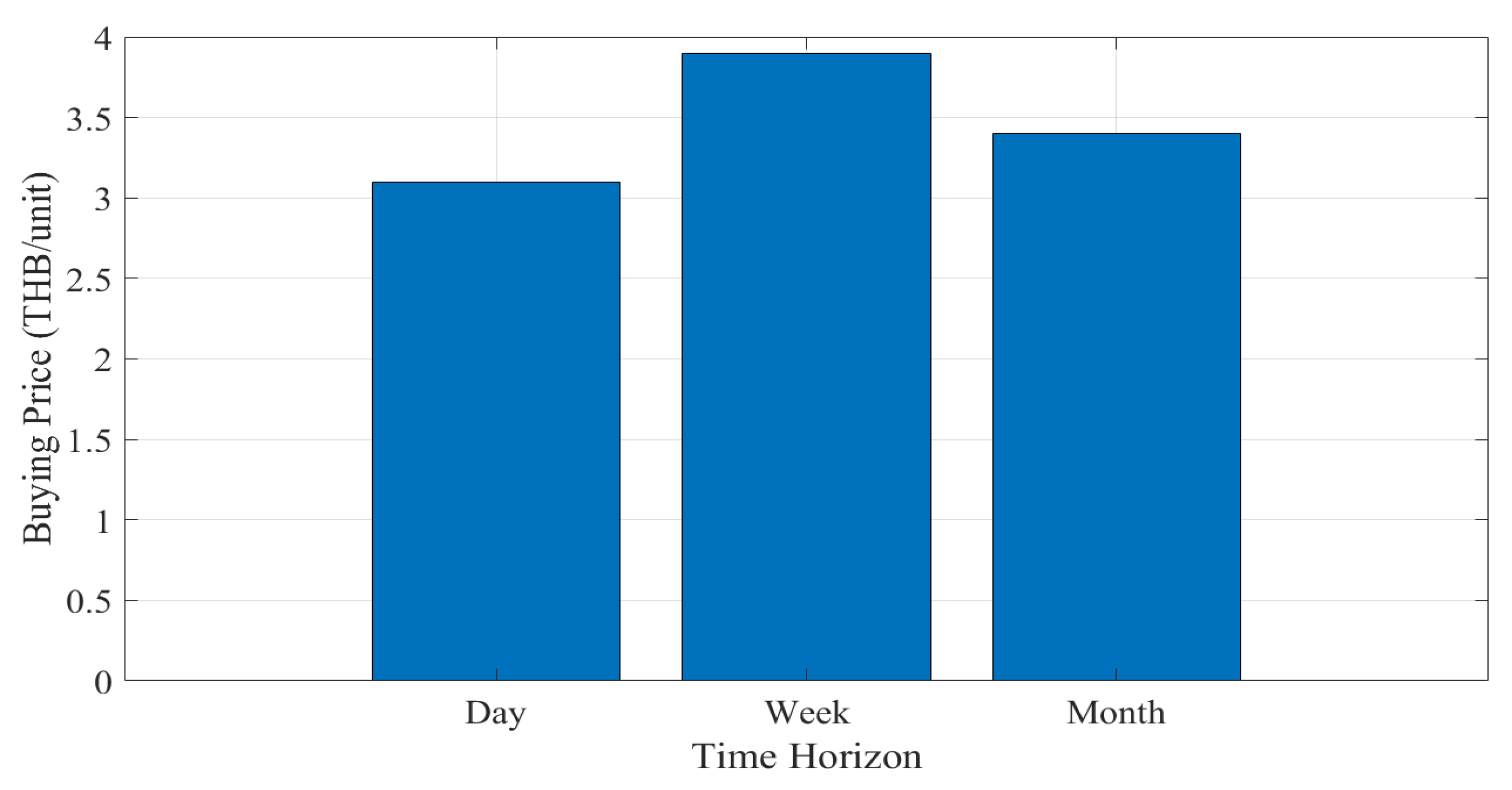
Figure 20 presents the optimal buying price (in THB per unit) for the energy aggregator under three different planning horizons: daily, weekly, and monthly. The variable $p_{buy}$ plays a critical role, as it indicates whether the proposed model can offer a more cost-effective alternative to traditional grid-based systems. The results reveal a clear variation in the optimal $p_{buy}$ across different time horizons.

For the daily horizon, the aggregator achieves a relatively low optimal price of approximately 3.1 THB per unit. However, as the planning horizon extends to one week, the optimal price increases to around 3.9 THB per unit. This rise is primarily due to the shorter simulation period and the greater variability in load demand caused by differing daily load profiles, which limits the optimizer’s ability to adjust to fluctuations in PV generation. As a result, the model increases $p_{buy}$ to satisfy the budget balance constraint. In the monthly scenario, the price decreases to 3.4 THB per unit, reflecting improved adaptation and smoothing of variability over a longer period.

These results indicate that the optimal $p_{buy}$ value is sensitive to the length of the planning horizon. The daily horizon enables more precise adjustments and efficient energy dispatch by leveraging short-term data, resulting in a lower buying price. In contrast, the weekly horizon introduces greater variability and uncertainty, requiring a higher price to ensure financial stability and satisfy operational constraints. The monthly horizon provides a more comprehensive view of demand and generation patterns, allowing for better load averaging and a modest reduction in $p_{buy}$ compared to the weekly case.

This trade-off between time horizon and cost-efficiency underscores the importance of designing appropriate energy pricing strategies. While weekly optimization may lead to higher costs due to limited flexibility and aggregated risks, monthly strategies regain a degree of efficiency, although not to the extent achieved by daily operations. These findings highlight the value of adaptive and horizon-aware energy management approaches in achieving both cost minimization and operational reliability. In this context, the comparison of 1-day, 7-day, and 30-day planning horizons serves as a sensitivity analysis on temporal resolution, revealing how the choice of optimization window length directly influences the optimal battery size, PV capacity, and electricity buying price.

In addition to solution quality, the practicality of the optimization model in real-world scenarios also depends on computational efficiency. The MILP-based optimization model demonstrated efficient performance across all tested time horizons. Implemented in MATLAB (R2024b) and solved using the intlinprog solver on a consumer-grade laptop (Intel Core i7, 16 GB RAM), the model solved the daily (24-step) case in approximately 5 s, the weekly (168-step) case in 10 to 30 s, and the monthly (720-step) case in 30 s to 1 min. These relatively low computation times suggest the model is practical for offline analysis and planning in small-scale community energy systems. However, as the number of households or time steps increases, the MILP formulation’s computational complexity may rise significantly. This highlights the importance of exploring scalability in future work, particularly for real-time applications or larger communities. Possible directions include rolling-horizon frameworks, constraint reduction, upgrading computer specifications, or metaheuristic optimization methods to maintain tractability without sacrificing solution quality.

5.6. Impact of Battery and PV Size on Buyback Price

Figure 21 and Figure 22 illustrate the variation of $p_{buy}$ across different BESS and PV sizes for three time horizons: daily, weekly, and monthly. A consistent pattern is observed in all cases. Specifically, $p_{buy}$ follows a convex curve (inverted bell shape) with respect to BESS size and exhibits a generally decreasing or flat trend with respect to PV size.

In the BESS size simulations, $p_{buy}$ initially decreases, reaching a minimum around 50 kWh, where the system achieves cost-effective energy shifting. For example, under the daily scenario, $p_{buy}$ drops from 3.3 THB per unit at 1 kWh to approximately 3.1 THB per unit at 50 kWh. Beyond this point, the value of $p_{buy}$ steadily increases, reaching over 5.4 THB per unit at 300 kWh. This increase reflects the higher capital cost and underutilization of excess storage capacity. A similar convex trend is observed in both the weekly and monthly cases.

The notably higher battery capacity requirement in the weekly horizon can be attributed to greater variability and uncertainty in solar generation and household demand over a seven-day period. To maintain energy balance and minimize grid imports during high-cost periods, the system must store excess PV energy during low-demand hours and discharge it during peak demand, necessitating a larger energy buffer. This explains why the weekly scenario results in the largest optimal battery size among the three.

In contrast, the daily horizon benefits from short-term predictability and fine-grained control, reducing the need for large storage. In this case, a battery size of only 60 kWh is sufficient to manage fluctuations between load and PV generation. The monthly horizon, despite spanning a longer duration, benefits from averaging effects over a 30-day period. This temporal smoothing enables more efficient dispatch planning, which reduces the need for extensive storage. As a result, the optimal battery size stabilizes at around 70 kWh in the monthly case.

For the PV size simulations, the results show that in the daily scenario, $p_{buy}$ decreases from 4.0 THB per unit at 1 kW to approximately 3.1 THB per unit at 3 to 4 kW, after which it stabilizes. A similar trend is observed in the weekly and monthly scenarios, where $p_{buy}$ declines from around 4.5 THB per unit to below 4.0 THB per unit as PV capacity increases beyond 5 kW. Beyond this threshold, further increases in PV size have little effect on reducing $p_{buy}$, primarily due to storage capacity limits and load saturation.

In summary, $p_{buy}$ is highly sensitive to battery oversizing and only moderately responsive to increases in PV capacity. The inverted bell-shaped curve observed with respect to BESS size highlights the optimal point where storage is effectively utilized without excess investment. These findings emphasize the importance of jointly optimizing PV and BESS capacities to maintain reasonable $p_{buy}$ values and ensure the long-term financial sustainability of the energy-sharing model. Based on the results, the optimal $p_{buy}$ value lies within the range of 3.2 to 3.4 THB per unit.

5.7. Robustness Analysis

To evaluate the reliability and robustness of the proposed SEAMS framework, multiple simulations were conducted under varying operational conditions. First, the model was tested across three planning horizons: daily, weekly, and monthly. As shown in Figure 18, Figure 19 and Figure 20, the daily and monthly results exhibit consistent trends in optimal PV sizing (6 kW per household), BESS capacity (60–70 kWh), and internal buying price ($p_{buy}$), demonstrating the model’s temporal stability in typical short- and long-term planning contexts. Although the weekly horizon produced higher system costs and slightly larger optimal battery sizes, this deviation reflects realistic mid-horizon aggregation effects and has been further discussed in Section 5.5. Second, the framework was applied to households with diverse load profiles, ranging from low to high demand. In all cases, the per-household cost scaled appropriately with consumption, while the energy allocation and pricing mechanism remained equitable. This confirms SEAMS’s ability to handle user diversity without compromising fairness or efficiency. Finally, all simulations converged to optimal solutions in under one minute on a standard laptop (Intel Core i7, 16 GB RAM), confirming the computational efficiency of the MILP formulation. Overall, while moderate deviations were observed in mid-term horizons, the SEAMS model consistently produced stable and realistic results across most planning scenarios and household types, affirming its robustness and suitability for practical implementation.

5.8. Scenario Comparison

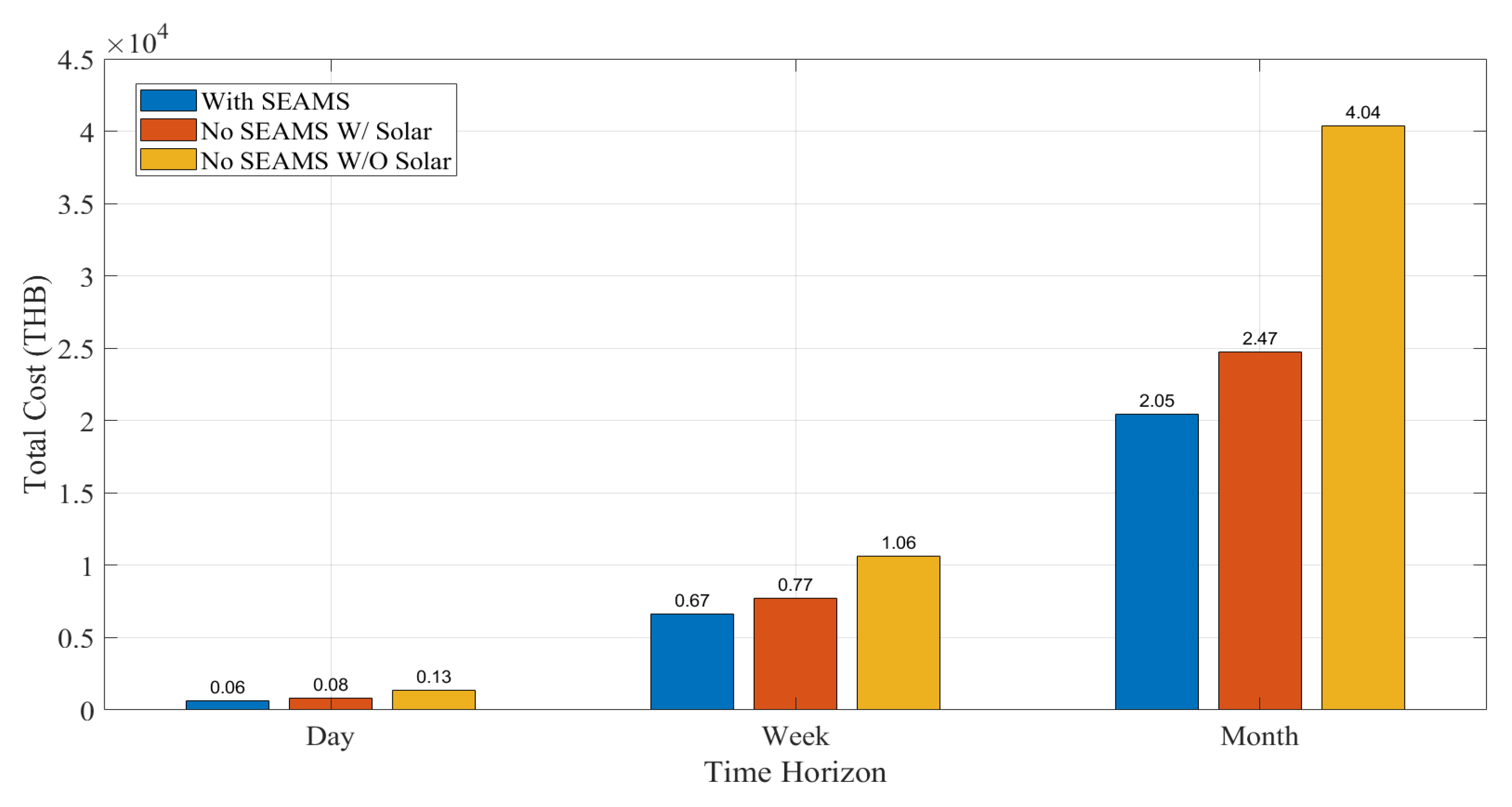
Figure 23 compares the total electricity cost under three frameworks: with SEAMS, without SEAMS but with solar, and without SEAMS and without solar, across three time horizons: daily, weekly, and monthly. The results clearly show that the proposed SEAMS consistently achieves the lowest total cost across all time scales. It is also evident that as the time horizon increases, the cost differences between scenarios become more pronounced. Based on the monthly horizon, the total electricity cost with SEAMS is 20,450 THB. This rises to 24,719 THB in the case without SEAMS but with solar, and peaks at 40,382 THB in the baseline case without both SEAMS and solar. These values correspond to a 16.9% cost reduction relative to the no-SEAMS-with-solar scenario, and a 49.4% reduction compared to the scenario without SEAMS and solar. The cost advantage offered by the SEAMS framework is also observed in the daily and weekly simulations, demonstrating its robustness and adaptability across different planning horizons. These findings confirm that the SEAMS model not only supports more cost-efficient energy management but also performs consistently under various temporal conditions.

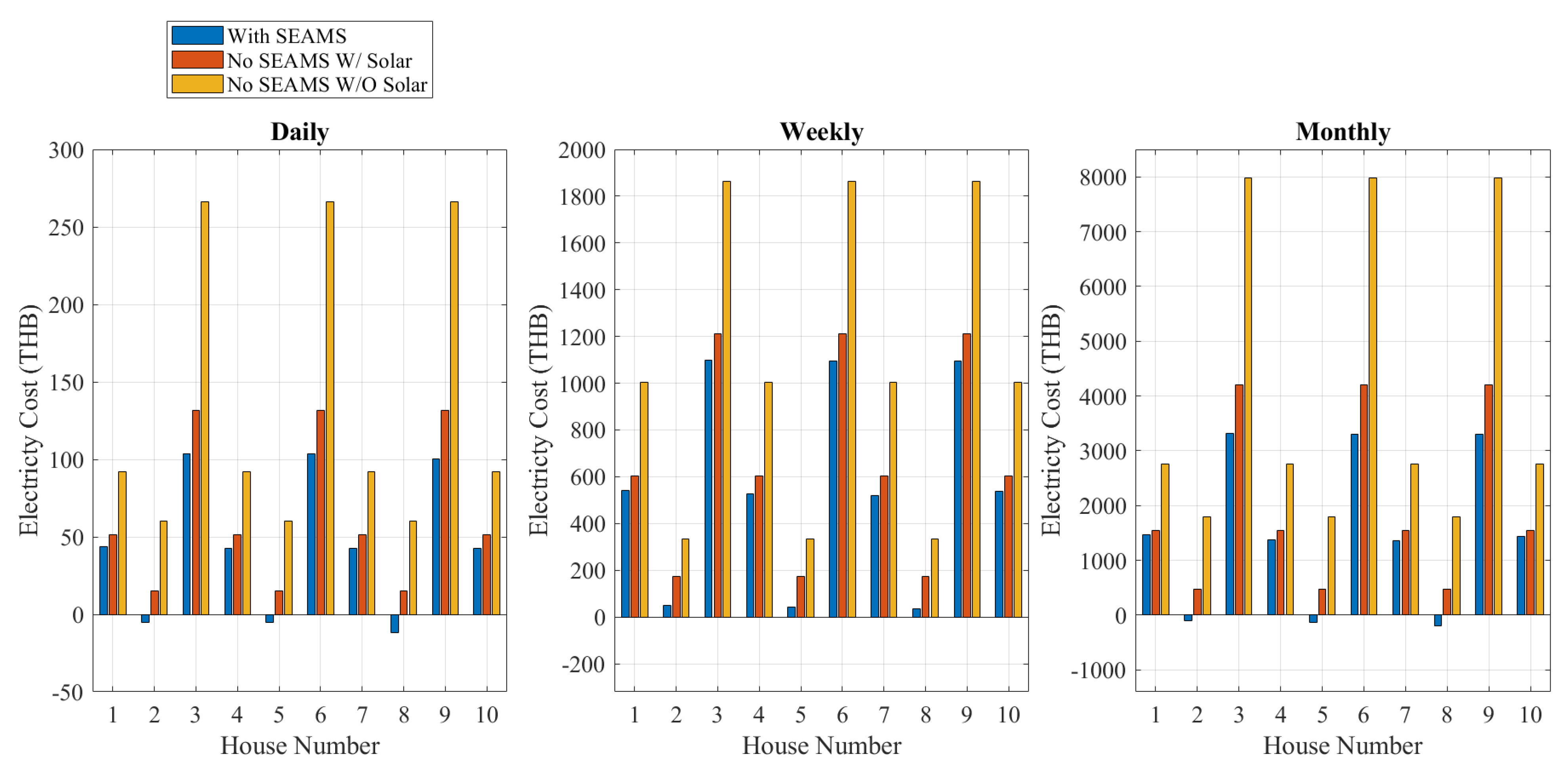
As shown in Figure 24, the SEAMS model consistently provides the lowest, and in some cases even negative, electricity costs per household across all time horizons. In the daily simulation, most households under the SEAMS model pay less than 100 THB per day. In contrast, electricity costs rise to approximately 130 THB per day in the scenario without SEAMS but with solar, and up to 270 THB per day in the scenario without both SEAMS and solar. Notably, low-load households experience negative electricity costs, indicating that they generated and sold more energy to the aggregator than they consumed, effectively earning a net profit. This outcome is the result of the net billing mechanism applied to every household, allowing residents to recover costs by selling surplus energy ($E_{sell,i}^t$) during the daytime. Consequently, household electricity bills are substantially reduced by the end of the month, as reflected in Figure 23 and Figure 24. The advantages of SEAMS become even more pronounced in the weekly and monthly simulations. In the monthly case, households without SEAMS and solar pay over 8000 THB, while those participating in the SEAMS model pay approximately 3400 THB. Some households even generate net income through excess energy sales. The reduction in electricity costs is consistent across all household types, demonstrating equitable savings and effective load balancing made possible by centralized energy management. This model shows strong potential for deployment in smart communities in Thailand, where reducing household energy expenditure and maximizing the use of local solar resources are important policy objectives.

Therefore, the MILP-based SEAMS framework offers significant improvements over conventional approaches by providing globally optimal energy management and high solar utilization. Compared to current practices (such as grid-only usage or uncoordinated solar consumption), SEAMS reduces total electricity costs by approximately 49% and 17%, respectively, across all simulated time horizons. The model adapts effectively to varying household loads, PV capacities, and operational durations, consistently outperforming static tariff and rule-based systems. Beyond cost efficiency, SEAMS introduces several structural advantages: fixed internal pricing, which promotes ease of adoption and user trust; shared battery storage (BESS) integrated via a centralized aggregator for flexible energy management; a budget-balanced operation model that ensures financial neutrality for the aggregator; a scalable MILP-based formulation that converges rapidly across daily, weekly, and monthly planning horizons; and compliance with real-world policy constraints, including the prohibition of residential grid exports and alignment with Thai TOU tariffs. These combined features ensure that all user types benefit equitably, reinforce SEAMS’s economic and operational feasibility, and support its potential deployment in Thai smart communities.

5.9. Impact of Prosumer Participation Level

As Thailand has not yet fully transitioned to renewable energy, achieving complete participation in such systems during the initial phase is challenging. To reflect this reality, the project simulates the total system cost and optimal BESS size under varying participation ratios, ranging from 10 percent to 100 percent. Figure 25 illustrates the results and highlights the trends as the level of participation changes. This represents a non-ideal case analysis aimed at understanding transitional dynamics, with the long-term goal of encouraging widespread adoption of the SEAMS framework in Thailand.

Across all time horizons, the total cost declines significantly as participation increases from 10 percent to 60 percent, with the most substantial cost reduction occurring at the lower participation levels. The cost trends follow a convex shape in all cases. For example, in the monthly simulation, the total cost drops from approximately 36,325 THB at 10 percent participation to around 19,040 THB at 60 percent participation, representing a 47.6 percent reduction. Beyond this point, the cost begins to plateau, indicating diminishing marginal savings as participation approaches 100 percent.

These findings suggest that full participation by prosumers may not be the most cost-effective configuration. A 60 to 40 ratio between prosumers and consumers appears to offer the optimal balance for the SEAMS model. At this ratio, the system achieves a sufficient level of self-generation capacity while maintaining enough consumer demand to absorb the surplus energy produced by prosumers. This leads to high self-consumption rates, reduced curtailment, and improved returns on investment in PV and storage systems. Beyond the 60 percent participation level, the marginal benefits begin to diminish due to saturation in generation and storage capacity. Retaining a portion of the community as consumers without PV contributes to balancing the load profile, supporting internal energy trading, and avoiding unnecessary infrastructure investment that yields limited additional benefits. This trend is consistently observed in both weekly and daily simulations, reinforcing the conclusion that broad but not complete participation enhances overall system efficiency and solar resource utilization within the SEAMS framework.

To contextualize the simulation range, the prosumer participation levels of 10% to 100% were selected to capture the full spectrum from limited early-stage adoption to a theoretical upper bound representing full community engagement. While 100% participation is not currently realistic, it serves as a benchmark to understand the system’s maximum potential under ideal conditions. In practice, Thailand’s rooftop PV adoption remains relatively low. As of 2020, approximately 3940 MWp of PV systems had been installed, of which 857 MWp were decentralized, grid-connected systems such as rooftop PV [65]. The estimated residential rooftop capacity by 2022 to 2023 reached about 1800 MWp, equivalent to just 1.6% of Thailand’s 21.7 million households [66], with total utilization still under 2% of the country’s 300 GW technical potential [66]. However, national policy and market trends indicate growing momentum. The AEDP 2015 to 2036 targets significant distributed energy expansion, and initiatives like the People’s Solar Project and EGAT’s “Energy is Yours” program [67] are enabling peer-to-peer energy trading in residential communities. Projections suggest that 25 to 40% of new residential developments will integrate rooftop PV by the early 2030s [68], with Thailand expected to become the second-largest solar market in ASEAN by 2036 [69]. In addition, several housing developments in Thailand have already begun adopting the SEAMS model of decentralized, community-based energy systems. At The Clouds III Hua Hin, for example, more than 70% of homes will be equipped with solar panels to promote energy-conscious living [70]. Other developments, such as Thai Country Homes’ Hua Hin Pool Villas, plan to install rooftop solar PV systems on every unit, with energy netted at the community level [71]. Furthermore, Sansiri, Thailand’s largest real estate developer, has committed to integrating solar rooftops on every unit across 31 new residential projects [72]. Simulating across a broad range of participation levels enables the model to evaluate both present-day dynamics and future policy-aligned scenarios.

5.10. Policy Suggestion

The findings of this study offer clear implications for energy policy in Thailand and similar developing countries. First, the results demonstrate that enabling internal community energy trading without grid export as modeled in SEAMS is both technically feasible and economically advantageous. This suggests that all regulatory bodies including the government such as the ERC, MEA, and PEA should support aggregator-led community models through dedicated legal frameworks, especially in contexts where feed-in tariffs or grid export permissions are restricted as this will increases the efficiency of P2P energy trading and also enhanced community total cost minimization as all energy will be utilized instead of wasted.

Second, the simulation results show that a fixed internal energy price can still achieve significant cost savings and fairness among households, which supports the implementation of simple, transparent pricing mechanisms for communities without requiring dynamic market-based tariffs. This aligns well with current policy goals focused on public trust and ease of participation.

Third, the identification of optimal PV (6 kW) and battery sizes (70–75 kWh) under realistic cost and load conditions highlights the need for updated technical guidelines and incentive programs tailored to shared infrastructure. Policymakers or the Thai government sector should consider revising existing rooftop solar subsidies or introducing targeted support for community-scale BESS deployment.

Lastly, the sensitivity analysis on prosumer participation suggests that partial participation models (60:40 prosumer-to-consumer ratio) can still yield substantial system-wide benefits. This supports a phased roll-out strategy that accommodates gradual adoption rather than requiring full participation from the outset. Therefore, pilot programs and regulatory sandboxes should be expanded to test and scale hybrid configurations across diverse communities, as all communities are not the same, and the model should adapt to the applied community.

By recognizing the demonstrated cost-effectiveness, fairness, and scalability of the SEAMS framework, policymakers can accelerate Thailand’s transition to a decentralized, renewable-powered future in a manner that is both inclusive and regulation-compliant.

5.11. Limitations

5.11.1. Hardware Limitations and Practical Considerations

Although the SEAMS framework includes a battery degradation cost based on the total energy charged and discharged, it uses a constant degradation coefficient and fixed charging/discharging efficiencies throughout the simulation period. These assumptions are appropriate for community-scale optimization studies and provide a reliable basis for evaluating cost-optimal system design under policy and pricing constraints. That said, real-world deployments in tropical environments like Thailand may introduce additional hardware considerations. High ambient temperatures and persistent humidity can accelerate battery aging, increase internal resistance, reduce storage efficiency, and shorten overall cycle life. During the monsoon season, elevated moisture levels may also contribute to corrosion in battery enclosures or power electronics, potentially affecting long-term performance and maintenance needs. Seasonal changes may impact short-term battery behavior as well. For instance, under hot and humid conditions, thermal losses may increase, and protective system features may limit charging or discharging power to maintain safe operation. While commercial battery systems in Thailand are typically designed to handle such conditions, these environmental effects are not explicitly modeled in this study.

To further improve realism and long-term planning accuracy, future work could incorporate temperature- and humidity-dependent degradation rates, along with efficiency variations tied to environmental conditions. Additionally, real-world installations may require protective infrastructure such as ventilation or climate-controlled enclosures, which could modestly increase investment or operational costs.

5.11.2. Economic Modeling Limitations

This study focuses on key investment and operational costs but acknowledges several simplifications in the economic modeling. Routine operation and maintenance costs for PV systems and batteries, such as inverter replacement or periodic cleaning, are not included since their impact on short-term dispatch is relatively minor. Battery replacement is not modeled as a discrete event. However, the battery investment cost is spread evenly over its expected lifetime (for example, 10 years), so that long-term ownership cost is proportionally reflected in the simulation. Policy incentives are also excluded to preserve a conservative, policy-neutral baseline. In Thailand, residential solar adoption still faces limitations. The People’s Solar Program, which is currently the main available incentive, involves a fixed 10-year contract at 2.2 THB per kilowatt-hour, limits installation size to 10 kW for 3-phase or 5 kW for 1-phase connections, and is subject to a national quota of 90 MW. The rate of 2.2 THB is considered relatively low compared to market electricity prices, making the program financially unattractive for many households. In this context, a locally managed solar village that aggregates and controls its own energy use, as modeled in this study, offers a more flexible and scalable alternative.

6. Conclusions

This paper investigates energy trading within a smart home community facilitated by a central aggregator (AGG), under regulatory constraints specific to the Thai context. In particular, the study considers practical policy limitations, including Thailand’s prohibition on exporting electricity back to the grid and the need to determine an appropriate fixed electricity price to promote user simplicity and trust. To address these challenges, the paper introduces SEAMS, a Solar Energy Aggregator Management System designed to optimize community energy trading. SEAMS integrates household photovoltaic (PV) generation, a shared Battery Energy Storage System (BESS), and an internal pricing mechanism managed by the central aggregator. The system achieves significant reductions in electricity costs through coordinated energy management. A mixed-integer linear programming (MILP) framework is employed to jointly optimize PV sizing, BESS capacity, and the internal buying price ($p_{buy}$) across various scenarios, including different time horizons and community participation levels.

Simulation results indicate that a PV capacity of 6 kilowatts and a BESS size of 70 to 75 kilowatt-hours offer the lowest total system cost under the solar irradiance and load conditions used in this study. However, these optimal sizes are dependent on specific load and PV generation profiles and may vary across regions. Moreover, a 60 to 40 ratio of prosumers to consumers is shown to provide the most effective balance between cost savings and efficient energy distribution. SEAMS enables cost reductions of up to 49 percent compared to traditional grid-only systems, with some households even achieving negative electricity costs through net billing. These outcomes position SEAMS as a practical, scalable, and policy-compliant model for advancing solar energy adoption and improving energy equity in Thailand. It lays a strong foundation for smart village development and supports national objectives for energy decentralization and long-term sustainability.

For future research, the SEAMS framework can be extended to simulate larger communities by adapting household demand and PV generation profiles to reflect different regions in Thailand and other countries. While this paper presents a generalized case study to validate the model and analyze system trends, future studies may apply SEAMS to diverse climate conditions and varying regulatory environments. This will support broader implementation of decentralized energy trading and enhance the system’s applicability across different socio-technical contexts. In addition, future work will involve validating the SEAMS framework using real-world data collected from actual smart community pilot sites in Thailand. This includes incorporating measured household demand, PV output, and battery behavior under local climate conditions. Such empirical validation will help refine key parameters, improve model accuracy, and ensure the simulation outcomes closely reflect real-world performance.