Abstract
Due to their simple design and reliable operation, earth-to-air heat exchangers (EAHE) are used in modern buildings to reduce ventilation heat losses. EAHE operation in atmospheric conditions results in variation in ambient air temperature and pressure affecting air density. The paper presents the study on the impact of ambient air density variation on the calculated hourly air temperature at the EAHE outlet and the resulting energy use for space heating and cooling of an exemplary residential building. The ground temperature was computed from the model given in EN 16798-5-1. Then, air density was obtained using five various methods. Energy use for space heating and cooling of the building was computed using the 5R1C thermal network model of EN ISO 13790. Depending on the chosen method and concerning the base case without EAHE, a reduction in annual heating and cooling needs was obtained from 7.5% to 8.8% in heating and from 15.3% to 19% in cooling. Annual heating and cooling gain from EAHE were 600.9 kWh and 628.3 kWh for heating and 616.9 kWh and 603.5 kWh for cooling for the Typical Meteorological Years (TMY) and International Weather for Energy Calculation (IWEC) files, respectively. Unit heating and cooling gains per heat exchanger area were from 34.9 kWh/m2 to 36.8 kWh/m2 and from −35.1 kWh/m2 to −36.3 kWh/m2. Density variation with temperature from the relevant typical Polish meteorological year at constant pressure, in comparison to the method of EN 16798-5-1, resulted in an hourly difference of that unit gain up to 4.3 W/m2 and 2.0 W/m2 for heating and cooling, respectively. The same was true inthe case of IWEC files that resulted in differences of 5.5 W/m2 and 1.1 W/m2.
1. Introduction
Energy consumption in buildings is of special interest at the national level in many countries due to the economic and environmental reasons [1]. In total, energy demand space heating and cooling have the most significant share [2,3,4]. Its value depends on several components. One of them, regardless of the building’s energy standard, is energy for heating and cooling ventilation air [5,6,7]. Since ventilation works all year round for hygienic reasons, supplying fresh outdoor air while removing polluted indoor air, its operation significantly affects the thermal demand of a building. Consequently, additional energy is needed for heating or cooling of air supplied to the interior of a building zone, in the cold and warm seasons, respectively.
To reduce the amount of that energy, various techniques of heat recovery from ventilation air are used, usually involving crossflow, counter-current or rotary heat exchangers [8,9]. However, together with the growing popularity of alternative and low-energy solutions, earth-to-air ground heat exchangers (EAHE, EAHX) have been gaining interest recently.
The design of EAHE should be performed carefully to avoid changes after it has been built, since correcting the position of a functioning device requires labour-intensive and costly earthworks. Therefore, numerous studies on the impact of various parameters on the EAHE performance were conducted, including climatic conditions and geographical location, soil type, pipe properties, burial depth and airflow rate [10]. In addition to experiments, theoretical analyses were carried out with the use of numerical simulations. As a result, methods of designing this type of heat exchanger have been developed for use in the heating and cooling of buildings in various climatic zones [11,12,13,14].
Since EAHEs are used commonly to reduce losses for heating or cooling the ventilation air, it becomes increasingly important to determine the energy effects of their application. Hence, calculation methods to assess the energy performance of EAHE are of growing significance. For this purpose, various tools have been used in recent studies.
D’Agostino et al. [15] analysed energy savings in an office building equipped with the HVAC system based on fan-coils and primary air, with and without EAHE and an air-to-air heat exchanger (AAHE). The authors used DesignBuilder and EnergyPlus to model the building and an HVAC system. They used the same set of tools in similar studies [16,17] on EAHE connected upstream with an air handling unit (AHU) and fan-coils in an office building. The EAHE model was validated with the two-dimensional finite element method and experimental data provided by other researchers.
Baglivo et al. [18] presented an hourly simulation of an air-cooled heat pump coupled with horizontal EAHE in a residential building. The hourly behaviour of EAHE was simulated in TRNSYS 17. Output results and relevant climatic data were used to compute calculate COP, EER, SCOP and SEER coefficients of the considered heat pump. The same tool was used in [19] to model various options of a ventilation system with EAHE in a residential building. The authors simulated the impact of the pipe numbers, air flow rate and soil thermal conductivity on the building thermal behaviour.
Other tools, as Ansys Fluent [20,21,22], Ansys CFX [23], Comsol Multiphysics [24], Matlab [25,26,27] or Scilab [28] were also used. However, although they offer great possibilities, their use requires specialised knowledge and experience. Hence, there is also a need for methods simpler but accurate enough to perform annual simulations with hourly time steps required by current standards and provide reasonable time resolution for thermal phenomena, occupation schedules, weather data and calculation accuracy [29,30,31], especially in terms of energy certification of buildings.
The EN 16798-5-1 standard [32], among others, gives the calculation method for preheating and precooling with necessary equations for ground temperature, temperature change in EAHE during airflow in the pipe and several auxiliary variables. The method is intended for use with hourly time steps. That standard has been used in several studies recently.
Skotnicka-Siepsiak [33] presented measurements of ground temperature and outlet air temperature of EAHE in a residential building in Olsztyn (northern Poland) in the warm months (May, June, July and August) of 2016, 2017 and 2018. Then, they were compared in the relevant charts with results based on EN 16798-5-1. The model provided comparable results for stable outdoor conditions in July and August. Larger differences were noticed in May and June.
Brata et al. [34] compared outlet temperature and monthly heat and cooling gains measured and calculated from EN 16798-5-1 for EAHE in an existing passive house near Timisoara in Romania. To assess the accuracy of the model authors used a histogram of residuals calculated as the difference between measured and calculated hourly values. They were between −0.9 °C and 2.8 °C. In general, monthly heat gains were slightly underestimated but monthly cooling energy was overestimated.
Michalak [35] coupled the model of EN 16798-5-1 with the thermal network model of a building zone from EN ISO 13790 [36] in an MS Excel spreadsheet to simulate in hourly time step an annual performance of EAHE connected with a ventilation system of a low-energy residential building in south Poland. In this way, hourly, as well as monthly and annual energy use for space heating and cooling and peak power with and without EAHE was estimated simply and efficiently.
It seems that due to its simplicity, this method does not offer as extensive possibilities as professional simulation programs. As mentioned above, they consider many physical properties. The most important of these include soil and pipe material parameters, flow rate and outside air temperature. They determine heat transfer conditions between soil and air flowing through a heat exchanger pipe from its inlet to its outlet. However, the above publications based on the standard model do not consider the influence of air temperature changes on air density [37], which in turn affects outlet air temperature from a heat exchanger. In [34] the air density was assumed constant. In [35,38] no information on the air density was given. Variation of thermal properties of air was considered in Comsol Multiphysics [24] and TRNSYS [38]. However, the review carried out shows that in most cases the authors used a fixed value for the air density and the specific heat of air. It was so in all types of tools, such as TRNSYS [19,39], Matlab [26,27] and Ansys [40,41]. There were also no studies comparing the assessment of these simplifications on outlet air temperature and resulting energy gain.
Therefore, this paper aims to present a detailed simulation study on the influence of changes in the air density and the specific heat depending on atmospheric conditions on a value of the temperature of outlet air from a heat exchanger. The method given in EN 16798-5-1 was used. To better illustrate the scale of the problem, based on the results obtained, the effect in the form of monthly and annual energy demand for heating and cooling of an example residential building was also determined. For this purpose, a well-known thermal resistance-capacitance model of a building zone given in EN ISO 13790 was used. As it is restricted only to sensible heating and cooling, the humidification and dehumidification processes of air were not considered here. Hence, the condensation in the buried pipe was also not analysed.
The following section presents the case building and climatic conditions in the considered location. Then the problem of thermal properties of air, in particular its density and specific heat capacity as a function of air temperature and atmospheric pressure are briefly presented. Moreover, the simulation models to obtain hourly outlet air temperature from EAHE and heating and cooling energy were presented. After them, the results are presented and compared with other studies, and concluding remarks are given.
2. Materials and Methods
2.1. Case Building
For further consideration, a single-story residential building was selected, located in Kraków (south Poland) in the third Polish climatic zone, following the subdivision from zone I to V given in the PN-EN 12831 standard [42] presented in Figure 1.
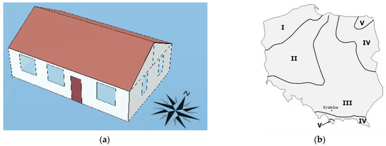
Figure 1.
(a) Model of the test building; (b) location of the building.
The building was built with traditional technology. It has external walls made of 25 cm ceramic blocks, insulated with 10 cm of Styrofoam. A 30° gable roof is isolated with a 15 cm layer of mineral wool. The ground floor was insulated with a 10 cm layer of Styrofoam. Following Polish requirements [43,44] ventilation airflow was set at 90 m3/h. The building has a total heated floor area of 65 m2, a total volume of 163 m3 and is inhabited by four people.
The mean annual temperature for the period 1971–2000 measured in the meteorological station Kraków-Balice and used to build a typical meteorological year (TMY) amounted to 8.20 °C and varied from 2.6 °C in February to 17.5 °C in July and August [45]. The hourly air temperature was from −20 °C on 16 February at 4:00 to 32.9 °C on 7 June at 12:00. Global horizontal solar irradiance was up to 998 W/m2 on 17 May at 11:00 (Figure 2).
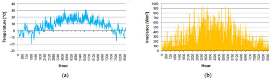
Figure 2.
TMY for Kraków: (a) outdoor air temperature; (b) global horizontal irradiance.
2.2. Earth-to-Air Heat Exchanger
As the design issues of EAHEs have been discussed by many researchers recently [23,24,46,47,48,49], these results were used to omit time-consuming preliminary considerations.
In the study [24] for Stockholm (Sweden) a 10 m long polyethylene pipe of 20 cm diameter, buried at 2 m was used for a volumetric airflow rate of 60 dm3/s (216 m3/h). For a residential building located in south Italy [50] authors considered 70 m long polypropylene pipes with a200 mm diameter buried at 1.50 m deep. In another case in a similar location [16] for an office building with a total floor area of 260 m2 and ventilation airflow rate of 1300 m3/h authors recommended EAHE from a pipe with 0.2 m diameter, between 80 m and 100 m long and buried between 2 m and 2.5 m. EAHE connected to a ventilation system of a single-family building in Poland presented in [51] consisted of two 25 m long parallel PVC 160/3.6 mm diameter pipes buried with increasing depth from 1.1 m up to 1.6 m at inlet and outlet, respectively. The ventilation airflow rate was 300 m3/h. The next one [33,52] was located in northern Poland. For a residential building with a usable floor area of 115 m2 and ventilation airflow rate of 150 m3/h EAHE was built from a 41 m long pipe with 0.2 m diameter buried at an average depth of 2.12 m.
Based on these experiences and the assumed ventilation rate of 90 m3/h, a 30 m-long pipe was chosen, with a diameter of 0.2 m and the burial depth set at 2 m. The main parameters of EAHE are given in Table 1. Assuming pipe wall thickness of 8.8 mm the inner surface area of the duct is As = 17.20 m2. Ground properties were taken from EN 16798-5-1.

Table 1.
Parameters of the earth-to-air heat exchanger.
The base for the EAHE performance simulation is the calculation of the hourly ground temperature at the burial depth. For this purpose, the method given in EN 16798-5-1 was used. Simplification assumptions of that model were given and discussed in [35,53,54,55]. The most important are as follows:
- –
- The ground is considered as a semi-infinite, homogenous and anisotropic medium,
- –
- The sinusoidal variation of ground surface temperature is assumed,
- –
- The model does not also take into account various environmental factors, as solar irradiance incident on a ground surface and periodic presence of snow cover on the ground.
- –
- The impact of EAHE operation on the ground temperature was omitted.
The hourly ground temperature is given by the expression:
The ξ factor is given by:
The time shift factor ft is expressed by the formula:
Finally, the difference between EAHE inlet and outlet air temperature (change in air temperature) can be computed:
Then, ventilation air at temperature:
is supplied to an interior of a considered building.
The overall heat transfer coefficient of the EAHE is given in the EN 16798-5-1 standard by the relationship:
However, it should be pointed out here that this equation is incorrect. According to the heat transfer theory [56] the overall heat transfer coefficient for a cylindrical heat exchanger, assuming convection only on an internal surface is given per unit inner surface area of a pipe by the expression:
Finally:
Then, if all quantities in Equation (4) are expressed as given in “Symbols” section, i.e., Udu [W/m2K], As [m2], qv;sup [m3/s], ρa [kg/m3] and ca [J/(kg∙K)] the fraction in the power of e in Equation (4) is dimensionless. Physically both denominator and numerator are then heat fluxes.
The inside surface heat transfer coefficient is given by:
That standard indicates the possibility to set Tmd = Te to avoid iterative computations when applying Equation (9).
2.3. The 5R1C Model
The EN ISO 13790 standard introduced the thermal network model of a building zone built from five resistors and one capacitor (Figure 3). It is intended for calculations of sensible energy use for space heating and cooling. Therefore, humidification and dehumidification of air are not considered here. Consequently, condensation processes in the buried pipe of EAHE were not analysed.
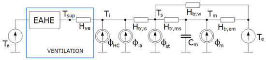
Figure 3.
The circuit diagram of the 5R1C thermal network model of a building zone with an earth-to-air heat exchanger to supply ventilation air.
That model was chosen for several important reasons as ease modification for various applications [57,58,59,60], low computational requirements [61,62,63] and its simplicity and possibility to apply in a spreadsheet [64,65,66] not requiring specialised commercial simulation tools while producing reliable results [67].
External partitions of a building are divided into two categories. The thermally light elements (doors, windows, curtain walls, glazed walls, etc.) are described by the Htr,w thermal transmission coefficient. The thermally heavy elements (walls, ceilings) are included in Htr,em and Htr,ms thermal transmission coefficients, both connected to the thermal capacity, Cm, representing the thermal mass of the building [68]. It is the weak point of this model since this way all the thermal inertia of various elements of a considered zone is considered as a single capacitance.
The ambient environment is represented by the external air temperature (Te). Htr,is is the coupling conductance between the central node (Ts) and an indoor environment (Ti).
Ventilation air, at temperature Tsup, is supplied to a building zone through the heat transfer by ventilation, Hve. To include the operation of EAHE its inlet and outlet were connected to Te and to Tsup, respectively. Tsup is calculated from Equation (5).
Heat fluxes from internal sources and solar radiation are split into three parts: φia, φst, and φm, connected to the indoor air, the central, and the thermal mass nodes, respectively. Heating or cooling power (φHC) is supplied to or extracted from the indoor air node. The calculation procedure to obtain heating and cooling power to maintain the required set point temperatures is given in EN ISO 13790 and has been presented in detail recently [69,70].
That procedure requires Tsup to be calculated at each time step. In the case when EAHE is not used and external air is directly supplied to a building then:
and ventilation heat flux is given by:
with the heat transfer by ventilation:
If EAHE is connected to the ventilation system, as shown in Figure 3, then an additional heat gain (or loss) is added to the heat exchanger during the flow of ambient air in the duct:
The supplying air temperature is calculated from Equation (5) and ventilation flux:
As presented in Equations (12)–(14), apart from the temperature difference, the product of ρa∙ca, called volumetric heat capacity of air, affects the calculated energy effect of ventilation and EAHE operation. Therefore, the dependence of these parameters on external conditions has to be carefully analysed and is presented in the next section.
Depending on the increase or decrease of the temperature of air passing the heat exchanger (ΔTsup > 0 or ΔTsup < 0), it is possible to talk about the heat or cold gain and to determine their monthly values. From this, including Equation (13), the monthly heat gain in EAHE in the m-th month is given by the expression:
Consequently, the monthly cooling energy gain in EAHE in the m-th month is given by the expression:
Thermal conductance and single capacitance of the RC network model (Figure 3) are given in Table 2. The thermal and physical properties of materials used were taken from manufacturers. Thermal resistances were calculated following ISO 6946 [71] Thermal bridges were neglected. Thermal capacities were calculated according to the detailed method of ISO 13786 [72] for the calculation period of 24 h. Solar absorptance of the roof and wall surfaces was: α = 0.8 and α = 0.6, respectively. Constant internal gains of 150 W throughout the year and continuous operation of the ventilation system were also assumed.
Table 2.
Thermal network model elements of the building.
EN ISO 13790 assumes constant volumetric heat capacity of air: ρaca = 1200 J/(m3K) as in other building simulations [52,68,73]. Hence, applying Equation (12) we get Hve = 30.0 W/K. This parameter was the same in all simulations to highlight the influence of the variation of air parameters on the operation of the analysed exchanger and not the whole exchanger-building system.
2.4. Thermal Properties of Dry Air in Building Simulations
Since, as stated in the introductory section, humidification and dehumidification of air is omitted in the present study, air shall be considered a dry gas. Within the air temperature and atmospheric pressure variation met in climatic conditions of inhabited areas around the globe it is sufficient to describe the atmosphere by the perfect gas law [74] linking together the absolute temperature (T), absolute pressure (p) and volume (V) for the given mass (M) of gas with a given individual gas constant (Ri):
Rearranging the above the unknown density can be calculated:
According to the International Union of Pure and Applied Chemistry (IUPAC) [75], we assumed the universal gas constant R = 8.3144598 J/(mol∙K) and molar mass of dry air μ = 28.96546 g/mol. Then, individual gas constant of dry air:
From this, at standard conditions defined by air temperature o T0 = 273.15 K (0 °C) and barometric pressure of p0 = 100 kPa at the sea level (altitude h = 0), we get:
In the same way, dry air density can be computed at a given hourly external (ambient) air temperature and pressure.
If the influence of variable atmospheric conditions on selected physical properties of air is to be considered, the most relevant independent variables and the ranges of their variability encountered in practice must be identified first. Taking into account WMO data [76] it seems reasonable to assume atmospheric pressure variation from 950 hPa to 1050 hPa and air temperature from −50 °C to +50 °C. The resulting air density variation for presented assumptions, calculated from Equation (18), is presented in Figure 4.
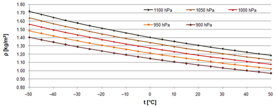
Figure 4.
Dry air density variation as a function of its temperature and atmospheric pressure.
Taking a pressure and temperature variation ranges from 950 hPa to 1050 hPa and from −20 °C to +20 °C, respectively, the air density varies from 1.12896 kg/m3 (950 hPa and +20 °C) to 1.44497 kg/m3 at 1050 hPa and −20 °C. In relation to 1.27540 kg/m3 at 0 °C and 1000 hPa it means the corresponding change of −13.0% and 13.3%.
If atmospheric pressure in a considered location is unknown then it can be calculated to the value at the known altitude from the barometric formula [77,78]. For ideal gas two forms of this equation exist [79]. The first one assumes the isothermal atmosphere, i.e., with a constant temperature independent on a height [80]:
and:
Hence, the air density, ρa,h, at a given altitude, h, is given by:
Standard conditions are used usually as reference. From this, assuming gravity acceleration g = 9.80665 m/s2, we get from Equation (23):
According to this equation the air density decreases from 1.27540 kg/m3 to 1.19808 kg/m3 (−6.1%), 1.12545 kg/m3 (−11.8%), and 0.99133 kg/m3 (−22.1%) at 500 m, 1000 m and 2000 m above sea level, respectively. However, since inhabited areas cover lands from 79 m below to 5516 m above sea level [81], these differences can be more significant when performing calculations for higher altitudes.
The second form of the barometric formula includes the lapse rate [82], i.e., the rate of decrease of temperature with a height. In the troposphere it amounts L = −6.51 K/km [83]. Then, in relation to sea level with h0 = 0 we get [84]:
and:
Density at altitude h is given by:
Inserting the aforementioned constants we get:
The EN 16798-5-1 standard recommends use of Equation (27) for Ta,ref = 20 °C and air density at sea level ρa,ref = 1.204 kg/m3 at p = 101,325 Pa. Hence, the above relationship is given in that standard in the following form:
Different values of the molar mass of air and universal gas constant were used in that standard which resulted in differences in the power (4.248 and 4.255) of expressions given by Equations (28) and (29).
According to Equation (29), for the given assumptions, air density decreases from 1.204 kg/m3 to 1.14811 kg/m3 (−4.6%), 1.09422 kg/m3 (−9.1%), and 0.99227 kg/m3 (−17.6%) at 500 m, 1000 m and 2000 m above sea level, respectively. Differences are lower than in the case of Equation (24) but still significant.
Application of Equation (23) at the temperature of 20 °C results in changes of density from 1.20413 kg/m3 to 1.13113 kg/m3, 1.06256 kg/m3 and 0.96734 kg/m3 in the same order. As the air temperature lapse rate is not included in this relationship, it produces results with the same percentage differences in relation to the sea level as for 0 °C for the same altitudes. A comparison of results from Equation (23) at 0 °C, Equation (23) at 20 °C and Equation (29) is given in Figure 5.
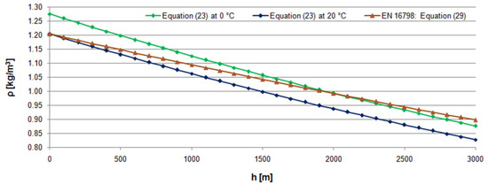
Figure 5.
Dry air density variation as a function of altitude.
The impact of air temperature and pressure on the specific heat capacity of air in atmospheric conditions is less significant [85] (Figure 6). Following correlations reported by Lemmon et al. [86] for dry air as an ideal gas, its specific heat at p = 101,325 Pa varies from 1006.03 J/(kg K) at 220 K (−53.15 °C) to 1007.41 J/(kg K) at 320 K (46.85 °C) with the minimum of 1005.68 J/(kg K) from 230 K to 280 K (from −43.15 °C to 6.85 °C). According to the next reference [87] at p = 100 kPa it varies from 1006.1 J/(kg K) at −50 °C to 1007.7 J/(kg K) at 50 °C with the minimum of 1005.7 J/(kg K) at −20 °C. Hence, in the considered range, the maximum value of ca is only 0.3% higher than the minimum in both cases, and for building energy simulation purposes its variation can be omitted using the constant ca = 1006.0 K/(kg K) [37].
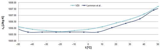
Figure 6.
Specific heat of dry air as a function of temperature.
For comparison, it should be noted that the EN 16798-5-1 standard imposes for the specific heat of air use of the constant value ca = 0.000279 kWh/(kg K) = 1004.4 J/(kg K), i.e., approximately 0.12% lower than the minimum values given.
3. Results and Discussion
3.1. Introduction
To present the problem of the air density variation with atmospheric conditions in the chosen location, several simulations were performed. They were based on the hourly data from the hourly typical meteorological year (TMY) for Kraków [45].
As described in [88] Polish TMYs do not include atmospheric pressure. Hence, it is necessary to determine the conditions for the meteorological station altitude using appropriate relationships. For comparison, the second source of meteorological data was also used. It was the International Weather for Energy Calculations (IWEC) weather data file for Kraków provided on the EnergyPlus website [89]. The IWEC weather files for over 200 locations around the world are freely provided by the U.S. Department of Energy [90,91].
It should be noted that air temperature in these two sources varies within a very similar range: from −20 °C to 32.9 °C and from −20.1 °C to 32.0 °C for TMY and IWEC files, respectively. Moreover, monthly values are very close (Figure 7a). However, hourly data differ more significantly (Figure 7b) as they are prepared from different source data.
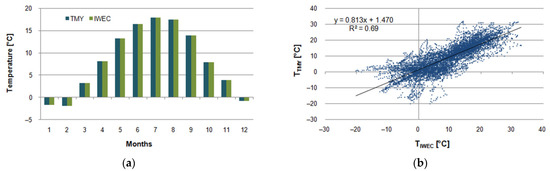
Figure 7.
Air temperature in Kraków according to weather data from TMY and IWEC: (a) monthly; (b) hourly.
Then, the hourly operation of EAHE at the same location was simulated assuming five methods:
- (1)
- Air density and specific heat of air from EN 16798-5-1, TMY;
- (2)
- Constant volumetric heat capacity of air from EN ISO 13790, TMY;
- (3)
- Air density from Equations (18) and (29) using the TMY data;
- (4)
- Air density from Equation (18) using the IWEC data;
- (5)
- Air density and specific heat of air from EN 16798-5-1, IWEC.
As the reference, the first case, i.e., the EN 16798-5-1 standard, was chosen as the recommended one for energy calculations of buildings in Poland. In the second case ρaca = 1200 J/(m3K) was used. In the third method, constant barometric pressure was obtained from Equation (29) and then varying air density was computed from Equation (18) using ambient air temperature from TMY. In the next method, as pressure and temperature are given in the IWEC file, air density was obtained from Equation (18). In the last method, air density was calculated following EN 16798-5-1 and the ambient air temperature was taken from the IWEC weather file. Hence, in relation to the previous case, there could be fully assessed the impact of the simplification introduced by that standard.
As the presented resistance-capacitance model of a building zone and the EAHE model are designed for calculations in hourly time steps they both were easily linked and simulated in a spreadsheet using hourly weather data for Kraków. This way no commercial program was necessary and an easily available tool was used.
3.2. Thermal Properties of Dry Air
At first, calculations following EN 16798-5-1 are presented. Meteorological station Kraków-Balice is located at the altitude of h = 237 m above sea level. Then from Equation (28) we get:
and resulting volumetric specific heat of air ρaca = 1182.43 J/(m3K). It is lower by about 1.5% from ρaca = 1200 J/(m3K) recommended by EN ISO 13790.
In the next step, assuming standard conditions given in Equation (18), from Equation (29) air pressure was calculated: p(h) = 97,071.05 Pa. Then, from Equation (18), hourly air density at the considered location, following air temperature variations, was obtained (Figure 8).
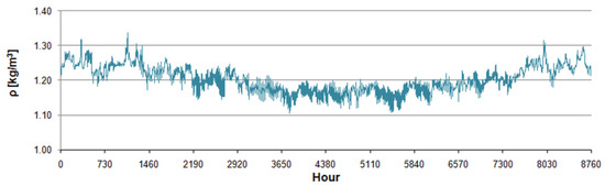
Figure 8.
Calculated air density.
It varied from 1.10495 kg/m3 on 7 June at 10:00 to 1.33691 kg/m3 on 16 February at 4:00, i.e., from −8.1% to 11.1% in relation to the annual average of 1.20286 kg/m3, which was only 2.1% higher than 1.177254 kg/m3 calculated following EN 16798-5-1. The monthly average density was from 1.1610 kg/m3 in June to 1.2504 kg/m3 in February.
The air density calculated from the IWEC weather file varied from 1.12822 kg/m3 on 8 July from 12:00 to 13.00 to 1.38083 kg/m3on 2 February at 6:00, i.e., from −7.9% to 12.7% in relation to the annual average of 1.22518 kg/m3 (Figure 9a). The monthly average density was from 1.1847 kg/m3 in August to 1.2704 kg/m3 in February. Hourly values differed from those of EN 16798-5-1 (Figure 9b).
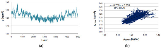
Figure 9.
Hourly air density for Kraków calculated from the IWEC data: (a) during the year; (b) correlation of hourly values in relation to the results from EN 16798-5-1.
Volumetric heat capacity for EN 16798 (method 1) amounted to 1182.43 J/(m3K). In the third method, the hourly value (dark green colour in Figure 10) was from 1111.58 J/(m3K) to 1344.93 J/(m3K) in comparison to the annual average of 1210.08 J/(m3K). Monthly averaged values were from 1167.95 J/(m3K) in June to 1257.87 J/(m3K) in February.
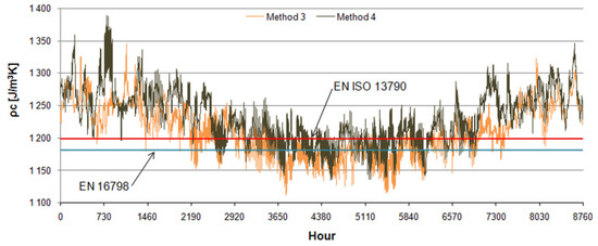
Figure 10.
Volumetric specific heat.
The last considered method produced values from 1134.99 J/(m3K) to 1389.12 J/(m3K) with 1232.53 J/(m3K) on average. Monthly averaged values were from 1191.85 J/(m3K) in July to 1277.98 J/(m3K) in February.
3.3. Performance of EAHE
To assess the effect of the considered methods on EAHE performance, we performed hourly simulations of the presented heat exchanger supplying ventilation air to the residential building.
As it could have been predicted from Equations (4) and (5), the influence of the density and specific heat variability on the temperature change in EAHE (ΔTsup) and outlet air temperature from EAHE (Tsup) are negligible. These predictions were confirmed by the results of the calculations. In the following paragraphs, they are given in relation to the first method, following Section 3.1, as used in energy calculations in Poland.
Outlet air temperature (Figure 11), calculated according to method (1), in the order presented in Section 3.1, varied from 0.93 °C on 16 February at 6:00 to 15.35 °C on 16 August at 15:00 (Figure 9). For method (2), it was from 0.90 °C on 16 February at 6:00 to 15.37 °C on 16 August at 15:00. In the next case, it was from 0.59 °C on 16 February at 6:00 to 15.25 °C on 16 August at 15:00. According to the fourth method, it varied from 0.65 °C on 3 February at 6:00 to 15.05 °C on 15 August at 15:00. In the last case, similar values were obtained, i.e., from 1.09 °C (3 February at 6:00) to 15.12 °C (15 August at 15:00). This shows that the baseline temperature varied within the same limits taking extreme values on the same days.
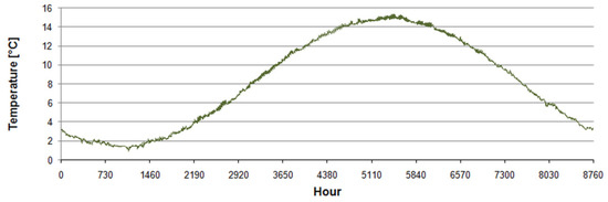
Figure 11.
Outlet air temperature (Tsup) from EAHE.
Hourly differences between calculated outlet values were also negligible. In relation to method (1), they were from −0.03 °C to 0.03 °C, from −0.02 °C to 0.34 °C, from −0.72 °C to 1.04 °C, and from −0.72 °C to 0.73 °C, respectively. Therefore, strong correlations between them were obtained (Figure 12 and Figure 13).
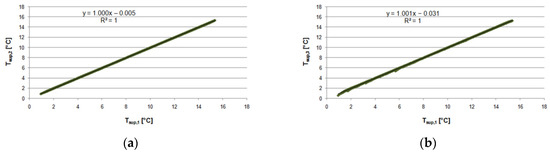
Figure 12.
Hourly outlet air temperature from EAHE from method (1) and: (a) method (2); (b) method (3).
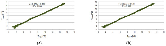
Figure 13.
Hourly outlet air temperature from EAHE from method (1) and: (a) method (4); (b) method (5).
For the subsequent methods hourly heat flux gain in EAHE varied following the temperature rise in EAHE (Equation (14)) and was from −631.4 W on 7 June at 12:00 to 638.4 W on 29 November at 6:00, from −639.8 W on 7 June at 12:00 to 646.9 W on 29 November at 6:00, from −597.2 W on 7 June at 12:00 to 704.2 W on 29 November at 6:00, from −546.4 W on 22 April at 15:00 to 721.2 W on 2 February at 6:00 and from −554.4 W on 22 April at 15:00 to 627.0 W on 2 February at 6:00.
Hourly differences in heating gain in relation to the first method were up to −8.4 W (20 December at 24:00), −74.4 W (16 February at 6:00), from −721.2 W (2 February at 6:00) to 595.6 W (16 February at 4:00) and from −627.0 W (2 February at 6:00) to 596.6 W (16 February at 5:00). In case of cooling these differences were up to 8.3 W, from −34.2 W (7 June at 12:00) to 3.8 W (1 February at 22:00), from −459.7 W (7 June at 12:00) to 483.1 W (4 August at 15:00), and from −461.0 W (7 June at 12:00) to 500.8 W (4 August at 15:00).
As it can be noticed the largest discrepancies were in the last case because of different meteorological datasets. However, from the point of air density variation the most interesting are two comparisons. The first is between methods 1 and 3, i.e., with constant air density and constant specific heat of air from EN 16798-5-1 and air density varying with ambient air temperature from TMY at constant pressure computed from the same standard (Figure 14). The second is a comparison between methods 5 and 4, both based on the IWEC datasets. These two comparisons should be considered the most important for the aim of this study. Thus, the hourly difference ina heating and cooling flux between the two last methods was up to −94.2 W (2 February at 6:00), and from 11.4 W (11 March at 12:00) to −18.2 W (8 July at 15:00), respectively (Figure 15).
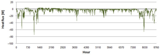
Figure 14.
Hourly differences of calculated heat flux from EAHE between methods 1 and 3.
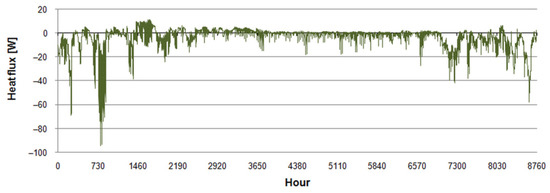
Figure 15.
Hourly differences of calculated heat flux from EAHE between methods 5 and 4.
The most significant differences are observed during periods with low outdoor air temperature, between −10 °C and −20 °C, i.e., when ventilation heat loss is significant and heating needs are high. Hence, the design of EAHE in such conditions should include the change in air density with ambient temperature.
Negative differences between simplified and more detailed methods mean that the use of constant air parameters from EN 16798-5-1 results in an underestimation of the resulting heat flux. In the considered cases this effect is especially visible at low outdoor temperatures during the heating period.
In the study [33] for Polish conditions, it was also concluded that the model of EN 16798-5-1 underestimated heat gain and overestimated cooling load. In [34] authors compared the same model and measurements and they stated that annual heating and cooling energy from the model was lower by 20–30% and greater by 8–20% than that from measurements, respectively.
As far as monthly (see Equations (15) and (16)) and annual aggregated values are considered, for the first three methods close monthly gains both for heating and cooling were obtained (Figure 16). However, the application of the last method resulted in more significant discrepancies. Monthly heat gain varied from 1 kWh in June to 128.7 kWh in November, from 1 kWh in June to 130.4 kW in November, from 1 kWh in June to 136.0 kWh in November, from 3.9 kWh in May to 128.5 kWh in December and from 3.7 kWh in May to 119.1 kWh in December.
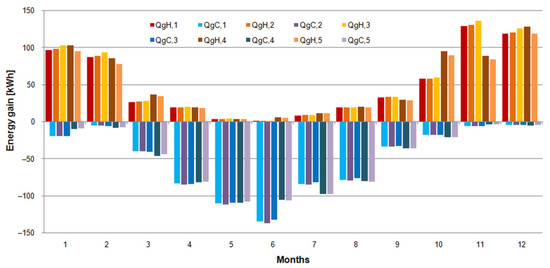
Figure 16.
Monthly heating and cooling energy gain in EAHE from methods 1–5.
Nevertheless, annual heat gains were quite similar and amounted to 600.9 kWh, 608.8 kWh, 632.4 kWh, 628.3 kWh and 586.1 kWh. In relation to the internal surface area of EAHE, the annual unit heat was 34.9 kWh/m2, 35.4 kWh/m2, 36.8 kWh/m2, 36.5 kWh/m2 and 34.1 kWh/m2.
In the case of cooling the situation was quite similar. Monthly cooling energy gain varied from −4.4 kWh in December to −135.0 kWh in June, from −4.5 kWh in December to −136.7 kW in June, from −4.5 kWh in December to 132.3 kWh in June, from −3.6 kWh in November to −109.5 kWh in May and from −3.5 kWh in November to −108.2 kWh in May. Annual gains amounted to −616.9 kWh, −625.0 kWh, −610.6 kWh, −603.5 kWh and −600.1 kWh. In relation to the internal surface area of EAHE, the annual unit heat was −35.9 kWh/m2, −36.3 kWh/m2, −35.5 kWh/m2, −35.1 kWh/m2 and −34.9 kWh/m2.
Simulation study for Swedish conditions [24] with a 10 m long polyethylene pipe of 20 cm diameter, buried at 2 m resulted in the estimated annual energy saving at 525 kWh and 300 kWh for heating and cooling season, respectively. It means the average gain per unit surface area of EAHE at 83.6 kWh/m2 and 47.8 kWh/m2.
Łuczak et al. [92] analysed various configurations of EAHE of EAHE connected with an air conditioning system in Polish conditions using the Rehau company program for the selection of ground heat exchangers. Unit heat gain per internal surface area of EAHE during the heating period (from 1 September to 31 March) was 40.7 kWh/m2, 35.2, kWh/m2, 34.2 kWh/m2, 34.1 kWh/m2 for the Tichelmanns’ system (200 mm diameter, 1330 m and 182 m long), for the meandering system (315 mm diameter and 120 m long) and for the ring system ((315 mm diameter and 120 m long), respectively.
Simulations of EAHE (5 m long pipe with a diameter of 200 mm and airflow rate of 150 m3/h) located in southern Italy with ANSYS Fluent, presented by Congedo et al. [93], resulted in a total monthly heat gain was from 8.95 kWh in February to 174.70 kWh in November and from −26.26 kWh in August to −167.67 kWh in July.
The experimental study of Skotnicka et al. [94] contains valuable comparative results from a laboratory experiment with EAHE conducted from 1 July to 30 September 2016 in Olsztyn (north Poland). To build EAHE a 41 m long polypropylene pipe with 0.2 m diameter was used. The maximum measured and calculated hourly heating and cooling gain was 0.29 kWh, 0.73 kWh, −0.16 kWh and −0.65 kWh, respectively.
Monthly measured heat gain was 37.24 kWh, 62.42 kWh and 82.41 kWh in July, August and September, respectively. Consequently, it means monthly unit heat gain per internal surface area of EAHE at 1.4 kWh/m2, 2.4 kWh/m2 and 3.7 kWh/m2. Total and unit gain for this period was 182.07 kWh and 7.07 kWh/m2, respectively. Calculated monthly heat gains were similar to measured values and amounted for the same months to 44.00 kWh, 58.27 kWh and 95.22 kWh. Hence, unit gains were 1.7 kWh/m2, 2.3 kWh/m2 and 3.7 kWh/m2.
Measured monthly cooling energy in the same months were−6.42 kWh, −4.45 kWh and −1.35 kWh with unit values of 0.25 kWh/m2, 0.17 kWh/m2 and 0.05 kWh/m2. Simulated values were several times greater: −57.58 kWh, −79.92 kWh and −88.32 kWh with unit energy of 2.2 kWh/m2, 3.1 kWh/m2 and 3.42 kWh/m2.
In the next study [34] authors experimentally analysed the hourly performance of EAHE built from the 35 m long pipe with the external and internal diameters of 200 and 185 mm, respectively. Measured annual heating and cooling energy was 1761 kWh and 1152 kWh in 2013 and 1410 kWh and 1063 kWh in 2014, respectively. It leads to energy gains per unit area of 86.6 kWh/m2, 56.6 kWh/m2, 69.3 kWh/m2 and 52.3 kWh/m2, respectively. Differences between measured and values calculated according to EN 16798-5-1 of heating, cooling and seasonal energy gain from EAHE were up to 49%, 59% and 79%, respectively.
When analysing the presented outcomes, there should be remembered that humidification and dehumidification processes inside the EAHE were ignored. This simplification is commonly included by other researchers for convenience [23,26,47,48,49].
However, Niu et al. [95] developed in Matlab the polynomial regression model for predicting the cooling capacity of EAHE including total, sensible and latent cooling capacity as a function of the air temperature, the air relative humidity, the air velocity at the inlet of EAHE, the tube surface temperature and the tube length and diameter.
The presented results showed that the air temperature along EAHE was independent of inlet air humidity. They also showed that in the case of low inlet air relative humidity, below 40%, no condensation along with the length of the tube occurred. Their study was devoted, however, only to cooling demand. In Polish conditions, where heating prevails, the situation can be different.
3.4. Energy Performance of the Building
To estimate the impact of EAHE operation on energy use for space heating and cooling of the considered exemplary residential building the necessary simulations were performed. To estimate the obtained energy effect, the base case was simulated without EAHE at first. Then, the following four cases with EAHE were considered.
In comparison to the base case (QH,0 and QC,0 in Figure 17), the introduction of EAHE resulted in visible energy savings in the considered case regardless of the chosen calculation method. It is especially clear in the months with dominant heating or cooling conditions. However, in varying ambient conditions (March, April, September, and October) and the thermal demand of the building changing during the day from heating to cooling and vice versa, the effect is not so obvious. Then it seems to be more beneficial to introduce a bypass to switch the intake of ventilation air between EAHE and outdoor air [35,50,51,96].
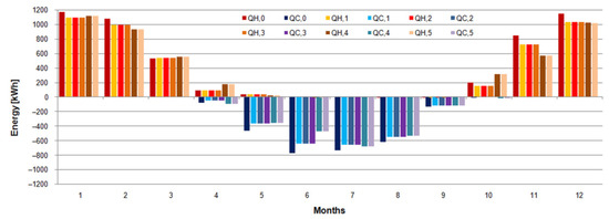
Figure 17.
Monthly energy use for space heating and cooling of the building.
Annual heating and cooling energy decreased from 5109 kWh and 2792 kWh in the base case to 4667 kWh and 2364 kWh, 4667 kWh and 2365 kWh, 4670 kWh and 2363, 4724 kWh and 2261 kWh, and 4719 kWh and 2261 kWh according to the successive methods, respectively. Hence, EAHE was responsible for the average annual reduction of 8.8% in heating and 15.3% in cooling energy in the first three methods. For the last one, reductions of 7.5% and 19.0% were obtained.
Figure 17 shows differences in calculated annual energy for space heating and cooling when using different weather datasets. For this reason, the weather files for energy simulations of buildings, especially in the case of energy certification, should be properly prepared. Moreover, atmospheric pressure should be included in Polish typical meteorological years.
Simulations in the Swedish climate [24] resulted in a 5% reduction for heating and a 50% reduction for cooling. In the case of a low-energy building located in Polish climatic conditions [35] EAHE reduced annual simulated heating and cooling needs by 13% and 43%, respectively. Results of long-term measurements of EAHE supplying ventilation air in a residential building located in north Poland presented in [33] showed annual savings of around 20% and 3% for heating and cooling energy, respectively.
The use of EAHE also improved the performance of the thermal energy source. Maximum heating and cooling power decreased significantly (Table 3). Only in the last case, it increase compared to the base case. It was caused by lower outdoor temperatures, especially on 2 February, when it varied from −20.1 °C at 7:00 to −4 °C at 14:00. The peak values of heating power in the remaining cases were noticed on 26 December when the outdoor air temperature was from −9.5 °C at 12:00 to −12.5 °C at 9:00. Moreover, unnecessary ventilation loss was reduced resulting in lower thermal demand for the building.
Table 3.
Maximum hourly heating and cooling power.
The next important aspect of this solution is the annual operation time of heating (τH) and cooling (τC). It was reduced in the cooling mode in all cases. In heating, it slightly increased, but the share of hourly power above 2000 W dropped rapidly (Figure 18 and Figure 19).

Figure 18.
Histograms of heating power: (a) the base case; (b) method 1.
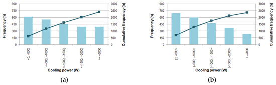
Figure 19.
Histograms of cooling power: (a) the base case; (b) method 1.
Presented histograms confirm a more stable operation of the heating and cooling source. In relation to the base case operation with heating and cooling power above 2000 W changed from 567 h to 210 h and from 396 h to 232 h. At the same time, power usage below 500 W increased: from 554 h to 611 h and from 618 h to 695 h.
4. Conclusions
In this study, the impact of air density variation with atmospheric conditions on the operation of the earth-to-air heat exchanger coupled with the ventilation system of the residential building in hourly time steps was studied.
As the Polish hourly typical meteorological years, available for 61 locations and intended for energy simulations of buildings, do not contain atmospheric pressure, the analysis took into account air density variation with ambient air temperature. The barometric pressure was computed as constant in relation to the reference conditions at sea level using the barometric formula at the altitude of the meteorological station. Therefore, air density variation analysis is limited only to one factor influencing its value—air temperature. In such a case, the density variation with temperature from the relevant weather files at constant pressure in comparison to the method of EN 16798-5-1 resulted in hourly differences in outlet air temperature up to 0.34 °C which can be treated as insignificant. Despite this, hourly differences in energy gain per unit area of the heat exchanger were up to 4.3 W/m2 and 2.0 W/m2 for heating and cooling, respectively.
For comparative purposes also the IWEC file was also used. However, as IWEC files are available only for four locations in Poland they are not used in practice. Instead, Polish TMYs are in common use as prepared for energy calculations of buildings both in monthly and hourly resolution. In this case, where both hourly ambient air temperature and atmospheric pressure were given, hourly differences in relation to the method using the same weather data but constant air properties from EN 16798-5-1 were up to 5.5 W/m2 and 1.1 W/m2 for heating and cooling, respectively.
These values seem not to be large, but analysed EAHE was rather small. So, in the case of larger objects hourly heating and cooling loads can differ more significantly. It was confirmed by comparisons of simplified methods with more detailed. In general, the model from EN 16798-5-1 underestimated heat gain and overestimated cooling load.
The presented considerations also confirmed the impact of the weather dataset used in calculations on monthly and annual energy gain from EAHE. The second one amounted to 600.9 kWh and 628.3 kWh for heating and 616.9 kWh and 603.5 kWh in cooling for the first and fourth methods (TMY and IWEC files), respectively. However, within the same weather data files it occurred that aggregated annual values of energy gain from EAHE were not significantly affected by simplifications regarding thermal properties of air, introduced both by EN 16798-5-1 or EN ISO 13790. As the influence of varying air density on ventilation loss and energy demand for heating and cooling of the building was not considered here, it may be analysed in a separate study.
The application of EAHE significantly decreased the energy demand for the heating and cooling of the building, by 8.2% and 16.8% on average, respectively.
As IWEC files are not used in energy audits or certification of buildings, it seems reasonable to introduce atmospheric pressure in typical Polish meteorological years. It would allow assessing the impact of air density variation on the EAHE performance.
This study shows the need to include atmospheric pressure in typical Polish meteorological years. Similarly, as in the case of heat load calculation following PN EN 12831, the design conditions for EAHE dimensioning in Polish climatic conditions could also be developed. It also indicates the need for future consideration about an assessment of air humidity impact on the simulated EAHE performance.
Funding
This research received no external funding.
Institutional Review Board Statement
Not applicable.
Informed Consent Statement
Not applicable.
Data Availability Statement
Not applicable.
Conflicts of Interest
The author declares no conflict of interest.
Symbols and Abbreviations
| As | inner surface of the ground heat exchanger, m2 |
| Cm | thermal capacity of the building, J/K |
| EA | unit heating and cooling energy use per unit area of a building, kWh/m2 |
| Htr,em | external part of the Htr,op thermal transmission coefficient, W/K |
| Htr,is | coupling conductance, W/K |
| Htr,ms | internal part of the Htr,op thermal transmission coefficient, W/K |
| Htr,op | thermal transmission coefficient for thermally heavy envelope elements, W/K |
| Htr,w | thermal transmission coefficient for thermally light envelope elements, W/K |
| Hve | thermal transmission coefficient by ventilation air, W/K |
| L | length of the duct, m |
| QC | annual energy use for space cooling, kWh |
| QgC,m | cooling energy gain in EAHE in m-th month, Wh |
| QgH,m | heating energy gain in EAHE in m-th month, Wh |
| QH | annual energy use for space heating, kWh |
| QHC | annual energy use for space heating and cooling, kWh |
| ΔQHC | percentage savings in annual energy use for space heating and cooling, % |
| Te | external (outdoor) air temperature, °C |
| Te;mn;an | mean annual temperature of outdoor air, °C |
| Te;max;m | maximum mean monthly temperature of outdoor air, °C |
| Tgnd | hourly ground temperature, °C |
| Ti | internal (indoor) air temperature, °C |
| Ti,C,set | set-point indoor air temperature for cooling, °C |
| Ti,H,set | set-point indoor air temperature for heating, °C |
| Tm | thermal mass node temperature, °C |
| Tmd | average air temperature in the duct, °C |
| Ts | central node temperature, °C |
| Tsup | supply air temperature, °C |
| ca | specific heat of air at constant pressure, J/(kg∙K) |
| cgnd | specific heat of the ground, J/(kg∙K) |
| di | inner diameter of the duct, m |
| do | outer diameter of the duct, m |
| ft | time shift factor, |
| hi | inside surface heat transfer coefficient, W/m2K |
| hm | number of hours in m-th month, |
| qv;sup | volumetric airflow rate, m3/s |
| tan | annual hour, with tan = 0 h at the beginning of the year; h |
| tan;min | the time of the year when the monthly mean outdoor temperature is minimal, h |
| v | air velocity in the duct, m/s |
| z | burial depth of the duct, m |
| Δτm | length of the month m, h |
| λgnd | thermal conductivity of the ground, W/(m∙K) |
| λdu | thermal conductivity of the duct, W/(m∙K) |
| ξ | damping factor, |
| ρa | air density, kg/m3 |
| ρgnd | ground density, kg/m3 |
| φint | heat flow rate due to internal heat sources, W |
| φsol | heat flow rate due to solar heat sources, W |
| φia | heat flow rate to internal air node, W |
| φst | heat flow rate to central node, W |
| φm | heat flow rate to mass node, W |
| φve | heat flow rate by ventilation, W |
| φEAHE | heat flow rate from EAHE, W |
| φC | cooling power supplied to or extracted from the indoor air node, W |
| φH | heating power supplied to or extracted from the indoor air node, W |
| φHC | heating or cooling power supplied to or extracted from the indoor air node, W |
References
- Buildings Performance Institute Europe. Europe’s Buildings under the Microscope. 2011. Available online: https://www.bpie.eu/wp-content/uploads/2015/10/HR_EU_B_under_microscope_study.pdf (accessed on 9 March 2022).
- Kesten, D.; Tereci, A.; Strzalka, A.M.; Eicker, U. A method to quantify the energy performance in urban quarters. HVACR Res. 2012, 18, 100–111. [Google Scholar] [CrossRef]
- Aksamija, A. Design methods for sustainable, high performance building facades. Adv. Build. Energy Res. 2016, 10, 240–262. [Google Scholar] [CrossRef]
- Kneifel, J.; O’Rear, E. Reducing the impacts of weather variability on long-term building energy performance by adopting energy-efficient measures and systems: A case study. J. Build. Perform. Simul. 2017, 10, 58–71. [Google Scholar] [CrossRef]
- Witkowska, A.; Krawczyk, D.A.; Rodero, A. Investment Costs of Heating in Poland and Spain—A Case Study. Proceedings 2019, 16, 40. [Google Scholar] [CrossRef]
- Chwieduk, D.; Chwieduk, M. Determination of the Energy Performance of a Solar Low Energy House with Regard to Aspects of Energy Efficiency and Smartness of the House. Energies 2020, 13, 3232. [Google Scholar] [CrossRef]
- Ballarini, I.; Costantino, A.; Fabrizio, E.; Corrado, V. A Methodology to Investigate the Deviations between Simple and Detailed Dynamic Methods for the Building Energy Performance Assessment. Energies 2020, 13, 6217. [Google Scholar] [CrossRef]
- Mardiana-Idayu, A.; Riffat, S.B. Review on heat recovery technologies for building applications. Renew. Sustain. Energy Rev. 2012, 16, 1241–1255. [Google Scholar] [CrossRef]
- Xu, Q.; Riffat, S.; Zhang, S. Review of Heat Recovery Technologies for Building Applications. Energies 2019, 12, 1285. [Google Scholar] [CrossRef]
- Abbaspour-Fard, M.H.; Gholami, A.; Khojastehpour, M. Evaluation of an earth-to-air heat exchanger for the north-east of Iran with semi-arid climate. Int. J. Green Energy 2011, 8, 499–510. [Google Scholar] [CrossRef]
- Tan, L.; Love, J.A. A Literature Review on Heating of Ventilation Air with Large Diameter Earth Tubes in Cold Climates. Energies 2013, 6, 3734–3743. [Google Scholar] [CrossRef]
- Greco, A.; Masselli, C. The Optimization of the Thermal Performances of an Earth to Air Heat Exchanger for an Air Conditioning System: A Numerical Study. Energies 2020, 13, 6414. [Google Scholar] [CrossRef]
- Pakari, A.; Ghani, S. Energy Savings Resulting from Using a Near-Surface Earth-to-Air Heat Exchanger for Precooling in Hot Desert Climates. Energies 2021, 14, 8044. [Google Scholar] [CrossRef]
- Peña, S.A.P.; Ibarra, J.E.J. Potential Applicability of Earth to Air Heat Exchanger for Cooling in a Colombian Tropical Weather. Buildings 2021, 11, 219. [Google Scholar] [CrossRef]
- D’Agostino, D.; Marino, C.; Minichiello, F. Earth-to-Air Versus Air-to-Air Heat Exchangers: A Numerical Study on the Ener-getic, Economic, and Environmental Performances for Italian Office Buildings. Heat Transf. Eng. 2020, 41, 1040–1051. [Google Scholar] [CrossRef]
- D’Agostino, D.; Esposito, F.; Greco, A.; Masselli, C.; Minichiello, F. Parametric Analysis on an Earth-to-Air Heat Exchanger Employed in an Air Conditioning System. Energies 2020, 13, 2925. [Google Scholar] [CrossRef]
- D’Agostino, D.; Esposito, F.; Greco, A.; Masselli, C.; Minichiello, F. The Energy Performances of a Ground-to-Air Heat Exchanger: A Comparison among Köppen Climatic Areas. Energies 2020, 13, 2895. [Google Scholar] [CrossRef]
- Baglivo, C.; Bonuso, S.; Congedo, P.M. Performance Analysis of Air Cooled Heat Pump Coupled with Horizontal Air Ground Heat Exchanger in the Mediterranean Climate. Energies 2018, 11, 2704. [Google Scholar] [CrossRef]
- Baglivo, C.; D’Agostino, D.; Congedo, P.M. Design of a Ventilation System Coupled with a Horizontal Air-Ground Heat Exchanger (HAGHE) for a Residential Building in a Warm Climate. Energies 2018, 11, 2122. [Google Scholar] [CrossRef]
- Ahmed, S.F.; Khan, M.M.K.; Amanullah, M.T.O.; Rasul, M.G.; Hassan, N.M.S. Performance assessment of earth pipe cooling system for low energy buildings in a subtropical climate. Energy Convers. Manag. 2015, 106, 815–825. [Google Scholar] [CrossRef]
- Ahmed, S.F.; Amanullah, M.T.O.; Khan, M.M.K.; Rasul, M.G.; Hassan, N.M.S. Parametric study on thermal performance of horizontal earth pipe cooling system in summer. Energy Convers. Manag. 2016, 114, 324–337. [Google Scholar] [CrossRef]
- Cao, S.; Li, F.; Li, X.; Yang, B. Feasibility analysys of earth-air heat exchanger (EAHE) in a sports and culture centre in Tianjin, China. Case Stud. Therm. Eng. 2021, 26, 101654. [Google Scholar] [CrossRef]
- Bisoniya, T.S.; Kumar, A.; Baredar, P. Energy metrics of earth–air heat exchanger system for hot and dry climatic conditions of India. Energy Build. 2015, 86, 214–221. [Google Scholar] [CrossRef]
- Havtun, H.; Törnqvist, C. Reducing Ventilation Energy Demand by Using Air-to-Earth Heat Exchangers. Part 1–Parametric Study. In Sustainability in Energy and Buildings; Hakansson, A., Höjer, M., Howlett, R., Jain, L., Eds.; Smart Innovation, Systems and Technologies; Springer: Berlin/Heidelberg, Germany, 2013; Volume 22. [Google Scholar] [CrossRef]
- Ahmadi, S.; Shahrestani, M.I.; Sayadian, S.; Poshitri, A.H. Performance analysis of an integrated cooling system consisted of earth-to-air heat exchanger (EAHE) and water spray channel. J. Therm. Anal. Calorim. 2021, 143, 473–483. [Google Scholar] [CrossRef]
- Akbarpoor, A.M.; Poshtiri, A.H.; Biglari, F. Performance analysis of domed roof integrated with earth-to-air heat exchanger system to meet thermal comfort conditions in buildings. Renew. Energy 2021, 168, 1265–1293. [Google Scholar] [CrossRef]
- Zhang, C.; Xiao, F.; Wang, J. Design optimization of multi-functional building envelope for thermal insulation and exhaust air heat recovery in different climates. J. Build. Eng. 2021, 43, 103151. [Google Scholar] [CrossRef]
- Molcrette, V.F.A.; Autier, V.R.B. New expression to calculate quantity of recovered heat in the earth-pipe-air heat-exchanger operating in winter heating mode. Arch. Thermodyn. 2020, 41, 103–117. [Google Scholar] [CrossRef]
- Hong, T.; Buhl, F.; Haves, P.; Selkowitz, S.; Wetter, M. Comparing computer run time of building simulation programs. Build. Simul. 2008, 1, 210–213. [Google Scholar] [CrossRef][Green Version]
- Piana, E.A.; Grassi, B.; Socal, L. A Standard-Based Method to Simulate the Behavior of Thermal Solar Systems with a Stratified Storage Tank. Energies 2020, 13, 266. [Google Scholar] [CrossRef]
- Patrčević, F.; Dović, D.; Horvat, I.; Filipović, P. A Novel Dynamic Approach to Cost-Optimal Energy Performance Calculations of a Solar Hot Water System in an nZEB Multi-Apartment Building. Energies 2022, 15, 509. [Google Scholar] [CrossRef]
- EN ISO 16798-5-1; Energy Performance of Buildings. Ventilation for Buildings Calculation Methods for Energy Requirements of Ventilation and Air Conditioning Systems (Modules M5-6, M5-8, M6-5, M6-8, M7-5, M7-8). Method 1: Distribution and Generation. International Organization for Standardization: Geneva, Switzerland, 2017.
- Skotnicka-Siepsiak, A. Operation of a Tube GAHE in Northeastern Poland in Spring and Summer—A Comparison of Real-World Data with Mathematically Modeled Data. Energies 2020, 13, 1778. [Google Scholar] [CrossRef]
- Brata, S.; Tănasă, C.; Dan, D.; Stoian, V.; Doboși, I.S.; Brata, S. Energy potential of a ground-air heat exchanger–measurements and computational models. Sci. Technol. Built Environ. 2021, 28, 84–93. [Google Scholar] [CrossRef]
- Michalak, P. Hourly Simulation of an Earth-to-Air Heat Exchanger in a Low-Energy Residential Building. Energies 2022, 15, 1898. [Google Scholar] [CrossRef]
- EN ISO 13790; Energy Performance of Buildings—Calculation of Energy Use for Space Heating and Cooling. International Organization for Standardization: Geneva, Switzerland, 2009.
- Michalak, P. Ventilation heat loss in a multifamily building under varying air density. J. Mech. Energy Eng. 2020, 4, 97–102. [Google Scholar] [CrossRef]
- Bouhess, H.; Hamdi, H.; Benhamou, B.; Bennouna, A.; Hollmuller, P.; Limam, K. Dynamic simulation of an earth-to-air heat exchanger connected to a villa type house in Marrakech. In Proceedings of the 13th Conference of International Building Performance Simulation Association, Chambéry, France, 25–28 August 2013. [Google Scholar]
- Ghaith, F.A.; Razzaq, H.U. Thermal performance of earth-air heat exchanger systems for cooling applications in residential buildings. In Proceedings of the ASME International Mechanical Engineering Congress and Exposition, Pittsburgh, PA, USA, 9–15 November 2018; pp. 1–12. [Google Scholar] [CrossRef]
- Badescu, V.; Isvoranu, D. Pneumatic and thermal design procedure and analysis of earth-to-air heat exchangers of registry type. Appl. Energy 2011, 88, 1266–1280. [Google Scholar] [CrossRef]
- Serageldin, A.A.; Abdelrahman, A.K.; Ookawara, S. Parametric study and optimization of a solar chimney passive ventilation system coupled with an earth-to-air heat exchanger. Sustain. Energy Technol. Assess. 2018, 30, 263–278. [Google Scholar] [CrossRef]
- PN-EN 12831-1:2017; Energy Performance of Buildings–Method for Calculation of the Design Heat Load-Part1: Space Heating Load. Polish Committee for Standardization: Warsaw, Poland, 2017.
- Ferdyn-Grygierek, J.; Baranowski, A.; Blaszczok, M.; Kaczmarczyk, J. Thermal Diagnostics of Natural Ventilation in Buildings: An Integrated Approach. Energies 2019, 12, 4556. [Google Scholar] [CrossRef]
- Sowa, J.; Mijakowski, M. Humidity-Sensitive, Demand-Controlled Ventilation Applied to Multiunit Residential Building—Performance and Energy Consumption in Dfb Continental Climate. Energies 2020, 13, 6669. [Google Scholar] [CrossRef]
- Ministry of Investment and Development. Data for Energy Calculations of Buildings. Typical Meteorological Years and Statistical Climatic Data for Energy Calculations of Buildings. Available online: https://www.gov.pl/web/archiwum-inwestycje-rozwoj/dane-do-obliczen-energetycznych-budynkow (accessed on 9 March 2022).
- Pfafferott, J. Evaluation of earth-to-air heat exchangers with a standardised method to calculate energy efficiency. Energy Build. 2003, 35, 971–983. [Google Scholar] [CrossRef]
- Chlela, F.; Husaunndee, A.; Riederer, P.; Inard, C. Numerical Evaluation of Earth to Air Heat Exchangers and Heat Recovery Ventilation Systems. Int. J. Vent. 2007, 6, 31–42. [Google Scholar] [CrossRef]
- Warwick, D.J.; Cripps, A.J.; Kolokotroni, M. Integrating Active Thermal Mass Strategies with HVAC Systems: Dynamic Thermal Modelling. Int. J. Vent. 2009, 7, 345–367. [Google Scholar] [CrossRef]
- Ralegaonkar, R.; Kamath, M.V.; Dakwale, V.A. Design and Development of Geothermal Cooling System for Composite Climatic Zone in India. J. Inst. Eng. Ser. A 2014, 95, 179–183. [Google Scholar] [CrossRef]
- Stasi, R.; Liuzzi, S.; Paterno, S.; Ruggiero, F.; Stefanizzi, P.; Stragapede, A. Combining bioclimatic strategies with efficient HVAC plants to reach nearly-zero energy building goals in Mediterranean climate. Sustain. Cities Soc. 2020, 63, 102479. [Google Scholar] [CrossRef]
- Trząski, A.; Zawada, B. The influence of environmental and geometrical factors on air-ground tube heat exchanger energy efficiency. Build. Environ. 2011, 46, 1436–1444. [Google Scholar] [CrossRef]
- Skotnicka-Siepsiak, A. An Evaluation of the Performance of a Ground-to-Air Heat Exchanger in Different Ventilation Scenarios in a Single-Family Home in a Climate Characterized by Cold Winters and Hot Summers. Energies 2022, 15, 105. [Google Scholar] [CrossRef]
- Gwadera, M.; Larwa, B.; Kupiec, K. Undisturbed Ground Temperature—Different Methods of Determination. Sustainability 2017, 9, 2055. [Google Scholar] [CrossRef]
- Larwa, B.; Gwadera, M.; Kicińska, I.; Kupiec, K. Parameters of the Carslaw-Jaeger equation describing the temperature distribution in the ground. Tech. Trans. 2018, 115, 67–78. [Google Scholar] [CrossRef]
- Larwa, B. Heat Transfer Model to Predict Temperature Distribution in the Ground. Energies 2019, 12, 25. [Google Scholar] [CrossRef]
- Bergman, T.L.; Lavine, A.A.; Incropera, F.P.; DeWitt, D.P. Fundamentals of Heat and Mass Transfer, 8th ed.; Wiley: Hoboken, NI, USA, 2018. [Google Scholar]
- Panão, M.J.N.O.; Santos, C.A.P.; Mateus, N.M.; da Graça, G.C. Validation of a lumped RC model for thermal simulation of a double skin natural and mechanical ventilated test cell. Energy Build. 2016, 121, 92–103. [Google Scholar] [CrossRef]
- Jayathissa, P.; Luzzatto, M.; Schmidli, J.; Hofer, J.; Nagy, Z.; Schlueter, A. Optimising building net energy demand with dynamic BIPV shading. Appl. Energy 2017, 202, 726–735. [Google Scholar] [CrossRef]
- Shen, P.; Braham, W.; Yi, Y. Development of a lightweight building simulation tool using simplified zone thermal coupling for fast parametric study. Appl. Energy 2018, 223, 188–214. [Google Scholar] [CrossRef]
- Costantino, A.; Fabrizio, E.; Ghiggini, A.; Bariani, M. Climate control in broiler houses: A thermal model for the calculation of the energy use and indoor environmental conditions. Energy Build. 2018, 169, 110–126. [Google Scholar] [CrossRef]
- Lauster, M.; Teichmann, J.; Fuchs, M.; Streblow, R.; Mueller, D. Low order thermal network models for dynamic simulations of buildings on city district scale. Build. Environ. 2014, 73, 223–231. [Google Scholar] [CrossRef]
- Horvat, I.; Dović, D. Dynamic modeling approach for determining buildings technical system energy performance. Energy Convers. Manag. 2016, 125, 154–165. [Google Scholar] [CrossRef]
- Elci, M.; Delgado, B.M.; Henning, H.M.; Henze, G.P.; Herkel, S. Aggregation of residential buildings for thermal building simulations on an urban district scale. Sustain. Cities Soc. 2018, 39, 537–547. [Google Scholar] [CrossRef]
- Tagliabue, L.C.; Buzzetti, M.; Marenzi, G. Energy performance of greenhouse for energy saving in buildings. Energy Procedia 2012, 30, 1233–1242. [Google Scholar] [CrossRef][Green Version]
- Fabrizio, E.; Ghiggini, A.; Bariani, M. Energy performance and indoor environmental control of animal houses: A modelling tool. Energy Procedia 2015, 82, 439–444. [Google Scholar] [CrossRef]
- Jędrzejuk, H.; Rucińska, J. Verifying a need of artificial cooling-a simplified method dedicated to single-family houses in Poland. Energy Procedia 2015, 78, 1093–1098. [Google Scholar] [CrossRef][Green Version]
- Fischer, D.; Wolf, T.; Scherer, J.; Wille-Haussmann, B. A stochastic bottom-up model for space heating and domestic hot water load profiles for German households. Energy Build. 2016, 124, 120–128. [Google Scholar] [CrossRef]
- Mora, T.D.; Teso, L.; Carnieletto, L.; Zarrella, A.; Romagnoni, P. Comparative Analysis between Dynamic and Quasi-Steady-State Methods at an Urban Scale on a Social-Housing District in Venice. Energies 2021, 14, 5164. [Google Scholar] [CrossRef]
- Bruno, R.; Pizzuti, G.; Arcuri, N. The Prediction of Thermal Loads in Building by Means of the EN ISO 13790 Dynamic Model: A Comparison with TRNSYS. Energy Procedia 2016, 101, 192–199. [Google Scholar] [CrossRef]
- Costantino, A.; Comba, L.; Sicardi, G.; Bariani, M.; Fabrizio, E. Energy performance and climate control in mechanically ventilated greenhouses: A dynamic modelling-based assessment and investigation. Appl. Energy 2021, 288, 116583. [Google Scholar] [CrossRef]
- ISO 6946:2017; Building Components and Building Elements—Thermal Resistance and Thermal Transmittance—Calculation Methods. International Organization for Standardization: Geneva, Switzerland, 2017.
- ISO 13786:2017; Thermal Performance of Building Components—Dynamic Thermal Characteristics—Calculation Methods. International Organization for Standardization: Geneva, Switzerland, 2017.
- Lomas, K.J. Architectural design of an advanced naturally ventilated building form. Energy Build. 2007, 39, 166–181. [Google Scholar] [CrossRef]
- Vestfálová, M.; Šafařík, P. Determination of the applicability limits of the ideal gas model for the calculation of moist air properties. EPJ Web Conf. 2018, 180, 02115. [Google Scholar] [CrossRef]
- Mohr, P.J.; Newell, D.B.; Taylor, B.N. CODATA Recommended Values of the Fundamental Physical Constants: 2014. J. Phys. Chem. Ref. Data 2016, 45, 043102. [Google Scholar] [CrossRef]
- Arizona State University. World Meteorological Organization’s World Weather & Climate Extremes Archive. Available online: https://wmo.asu.edu/content/world-meteorological-organization-global-weather-climate-extremes-archive (accessed on 4 March 2022).
- Berberan-Santos, M.N.; Bodunov, E.N.; Pogliani, L. On the barometric formula. Am. J. Phys. 1997, 65, 404–412. [Google Scholar] [CrossRef]
- Andrews, D.G. An Introduction to Atmospheric Physics; Cambridge University Press: Cambridge, UK, 2000. [Google Scholar]
- National Ocean and Atmosphere Administration. U.S. Standard Atmosphere 1976; Nation Ocean and Atmosphere Administration: Washington, DC, USA, 1976. Available online: https://www.ngdc.noaa.gov/stp/space-weather/online-publications/miscellaneous/us-standard-atmosphere-1976/ (accessed on 14 March 2022).
- Dubinova, A.A. Exact explicit barometric formula for a warm isothermal Fermi gas. Tech. Phys. 2009, 54, 210–213. [Google Scholar] [CrossRef]
- Cohen, J.E.; Small, C. Hypsographic demography: The distribution of human population by altitude. Proc. Natl. Acad. Sci. USA 1998, 95, 14009–14014. [Google Scholar] [CrossRef]
- Benenson, W.; Harris, J.W.; Stöcker, H.; Lutz, H. Handbook of Physics; Springer: New York, NY, USA, 2002. [Google Scholar] [CrossRef]
- Jacobson, M.Z. Fundamentals of Atmospheric Modeling, 2nd ed.; Cambridge University Press: Cambridge, UK, 2012. [Google Scholar] [CrossRef]
- Corstanje, A.; Bonardi, A.; Buitink, S.; Falcke, H.; Hörandel, J.R.; Mitra, P.; Mulrey, K.; Nelles, A.; Rachen, J.P.; Rossetto, L.; et al. The effect of the atmospheric refractive index on the radio signal of extensive air showers. Astropart. Phys. 2017, 89, 23–29. [Google Scholar] [CrossRef]
- Wagner, W.; Kretzschmar, H.J.; Span, R.; Krauss, R. D2 Properties of Selected Important Pure Substances. In VDI Heat Atlas; Springer: New York, NY, USA, 2010. [Google Scholar] [CrossRef]
- Lemmon, E.W.; Jacobsen, R.T.; Penoncello, S.G.; Friend, D.G. Thermodynamic properties of air and mixtures of nitrogen, argon, and oxygen from 60 to 2000 K at pressures to 2000 MPa. J. Phys. Chem. Ref. Data 2000, 29, 331–385. [Google Scholar] [CrossRef]
- Struchtrup, H. Properties and Property Relations. In Thermodynamics and Energy Conversion; Springer: Berlin/Heidelberg, Germany, 2014. [Google Scholar] [CrossRef]
- Michalak, P. Modelling of Solar Irradiance Incident on Building Envelopes in Polish Climatic Conditions: The Impact on Energy Performance Indicators of Residential Buildings. Energies 2021, 14, 4371. [Google Scholar] [CrossRef]
- World Meteorological Organization. Weather Data. Available online: https://energyplus.net/weather (accessed on 17 March 2022).
- Bellia, L.; Pedace, A.; Fragliasso, F. The role of weather data files in Climate-based Daylight Modeling. Sol. Energy 2015, 112, 169–182. [Google Scholar] [CrossRef]
- Costanzo, V.; Evola, G.; Infantone, M.; Marletta, L. Updated Typical Weather Years for the Energy Simulation of Buildings in Mediterranean Climate. A Case Study for Sicily. Energies 2020, 13, 4115. [Google Scholar] [CrossRef]
- Łuczak, R.; Ptaszyński, B.; Kuczera, Z.; Życzkowski, P. Energy efficiency of ground-air heat exchanger in the ventilation and air conditioning systems. E3S Web Conf. 2018, 46, 00015. [Google Scholar] [CrossRef]
- Congedo, P.M.; Lorusso, C.; De Giorgi, M.G.; Marti, R.; D’Agostino, D. Horizontal Air-Ground Heat Exchanger Performance and Humidity Simulation by Computational Fluid Dynamic Analysis. Energies 2016, 9, 930. [Google Scholar] [CrossRef]
- Skotnicka-Siepsiak, A.; Wesołowski, M.; Piechocki, J. Experimental and Numerical Study of an Earth-to-Air Heat Exchanger in Northeastern Poland. Pol. J. Environ. Stud. 2018, 27, 1255–1260. [Google Scholar] [CrossRef]
- Niu, F.; Yu, Y.; Yu, D.; Li, H. Heat and mass transfer performance analysis and cooling capacity prediction of earth to air heat exchanger. Appl. Energy 2015, 137, 211–221. [Google Scholar] [CrossRef]
- Romanska-Zapala, A.; Bomberg, M.; Dechnik, M.; Fedorczak-Cisak, M.; Furtak, M. On Preheating of the Outdoor Ventilation Air. Energies 2020, 13, 15. [Google Scholar] [CrossRef]
Publisher’s Note: MDPI stays neutral with regard to jurisdictional claims in published maps and institutional affiliations. |
© 2022 by the author. Licensee MDPI, Basel, Switzerland. This article is an open access article distributed under the terms and conditions of the Creative Commons Attribution (CC BY) license (https://creativecommons.org/licenses/by/4.0/).