Abstract
The power grid has the characteristics of a weak grid with an increase in new energy penetration in the power system. Power electronic-based renewable generation brings issues that weaken the entire system, including the loss of inertia. Low inertia and weak damping cause system oscillation. Virtual synchronous generator (VSG) technology gives power electronic equipment inertia-support capability but increases the complexity of control system parameter design. Many researchers have studied the design method of VSG considering the frequency disturbance of the power grid. The traditional VSG parameter design method ignores the influence of source-side and grid-side fluctuations on the transient stability of the system, resulting in the difference between the actual dynamic and static indicators and the design indicators of VSG in a weak grid. This paper analyzes a small-signal model based on power fluctuations and frequency fluctuations and proposes a control parameter design method that combines the influence of grid impedance to ensure the dynamic stability of the system under a weak power grid. The simulation and experimental results verify the correctness and feasibility of the control method.
1. Introduction
The parameters of the VSG (Virtual Synchronous Generator) are crucial to the stability and dynamic performance of the system. In recent years, the design of control parameters has been discussed in many pieces of literature. The active power loop of VSG is a second-order control system, and its damping ratio affects the stability and dynamic performance of the system [1,2,3]. If the damping ratio is too small, it will cause serious active power oscillation, and if the damping ratio is too large, it will reduce the inertia of the system, which is not conducive to maintaining frequency stability. References [4,5] deduce the constraint relationship between the moment of inertia and the damping coefficient and repeat the trial and error process according to the constraint relationship, and the design process is complicated. Reference [6] analyzes in detail the influence of the active power control loop parameters on the system when the VSG stand-alone is connected to the grid, and adopts the “second-order optimal” system to tune the relevant parameters, but does not consider the frequency-modulation performance of the VSG. Reference [7] studies the parallel stability of VSG multi-machines and their off-grid switching and proposes a parameter design method that can improve system stability. Reference [8] proposed a complete set of parameter design methods for virtual synchronous generators using the control variable method to obtain parameter optimization by judging and analyzing the overshoot and response speed of the system response. References [9,10] studied the influence of the double power frequency ripple of the instantaneous output power on the output voltage during asymmetric operation and ensured the steady-state and dynamic performance of the system by limiting the cut-off frequency and phase angle margin of the power loop, but only the stability of the VSG under the rated operating point of the grid was analyzed, and the influence of fluctuations on the power supply side and the grid side was not considered. Reference [11] established the small signal model of VSG, obtained the phase angle margin constraints that the power loop decoupling needs to meet, and traversed the control parameters according to the constraints, which can meet the stability of the grid voltage change system.
In addition, many scholars have studied the VSG design method considering the power grid frequency disturbance. References [12,13] optimized the parameter design and improved the frequency stability of the system by studying the impact of virtual inertia and virtual damping of VSG on frequency stability. Reference [14] proposed a variable damping strategy by analyzing the influence of virtual synchronous generator damping on frequency stability but did not pay attention to the influence of other parameters on frequency stability. Reference [15] studied the influence of damping coefficient and moment of inertia on frequency stability and adopted an adaptive control strategy to suppress overshoot in the frequency transient process and improve frequency stability performance. Reference [16], in view of the inability of traditional virtual synchronous generators to suppress frequency oscillation, designed a frequency dividing sliding filter method according to different frequency bands, improved the virtual moment of inertia in sections, and adopted adaptive virtual damping to improve the adjustment ability of the system when frequency oscillation occurs. Reference [17] starts from the control model and transfer function, quantitatively analyzes the dynamic performance index in the time domain, and proposes a parameter design method that can adapt to the grid load disturbance and satisfy the frequency control index. Reference [18], based on the flexible virtual synchronous generator control technology of exponential inertia, through the construction of a small signal model, sensitivity calculation, and root-trajectory analysis, revealed the influence law of the main control parameters on the frequency stability of the system and provided a basis for the selection of control parameters.
The above traditional VSG parameter design method ignores the influence of power- supply-side and grid-side fluctuations, but with the gradual transition of the power grid from a strong power grid to a weak power grid, the influence of grid impedance is increasingly serious. The change of grid impedance not only threatens the stability of the grid-connected inverter but also affects the response speed of the virtual synchronous generator and the overshoot in the dynamic process. Therefore, how to adjust the control parameters of a virtual synchronous generator based on the impedance of the grid is a problem worth discussing [19,20].
In this paper, firstly, the active power-frequency and reactive power–voltage characteristics of the generator are analyzed; then, through small-signal modeling, the influence of grid frequency fluctuation and active power command fluctuation on the dynamic performance of the inverter is analyzed. Then, combined with the characteristics of a weak grid, the influence of virtual synchronous generator control parameters and grid impedance on the dynamic response performance of the system is analyzed through root locus and simulation, and the dynamic stability and dynamic response speed of the system are improved through optimization design. Finally, experimental verification is completed.
2. Basic Control Principle of Virtual Synchronous Generator
2.1. Active Power–Frequency Control Design
The system control circuit diagram of the virtual synchronizer is shown in Figure 1. The control section mainly includes the virtual synchronizer power loop, the outer voltage loop, and the inner current loop.
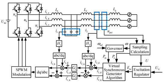
Figure 1.
Control circuit diagram of current-controlled virtual synchronizer system.
The condition for the system to maintain dynamic stability is that the electromagnetic power and mechanical power are kept in dynamic balance. When the dynamic balance is broken, the system will lose stability. For example, if the active load of the system increases suddenly at a certain moment, the electromagnetic power of the system increases accordingly. Due to the mechanical inertia of the rotor of the generator, the speed cannot change abruptly. Therefore, the mechanical power output of the synchronous generator is less than the electromagnetic power required by the load, resulting in a reduction in the frequency of the system [21]. When the governor of the synchronous generator is used for regulation, the frequency of the system can be stabilized near the rated frequency. The active power–frequency characteristic curve of the synchronous generator is shown in Figure 2a.
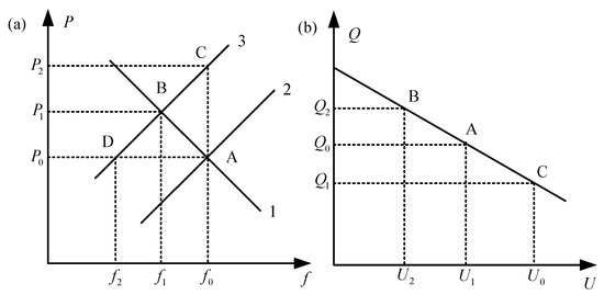
Figure 2.
Characteristic curve of synchronous generator. (a) Active power–frequency characteristic curve; (b) Reactive power–voltage static characteristic curve.
As shown in Figure 2a, curve 1 represents the power–frequency characteristic curve of the synchronous generator, and curves 2 and 3 represent the power–frequency characteristic curves for different active loads.
It can be seen from Figure 2a that the power–frequency static characteristic curve of the synchronous generator exhibits droop modulation characteristics [22] and can be expressed as:
where is the command value of mechanical power, is the actual output active power, is the reference value of generator angular frequency, is the rated angular frequency, and is the frequency regulation coefficient of generators.
The larger the value of , the smaller the deviation of the frequency will be.
From (1), the control block diagram of the governor can be obtained, as shown in Figure 3.
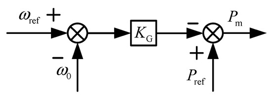
Figure 3.
Control block diagram of synchronous generator governor.
The active power–frequency control block diagram of the virtual synchronous generator is in Figure 4. The virtual synchronous generator does not have a real rotor, and the rotor parameters are not fixed. Through the proper design of the rotational inertia J and damping coefficient D, the system can obtain a faster dynamic response and a wider adjustment range.
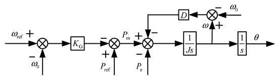
Figure 4.
Active power–frequency modulation loop structure block diagram.
2.2. Reactive Power–Voltage Control Design
Synchronous generators not only provide active power to the system through the governor but also provide reactive power to the system through the excitation regulator to maintain reactive power and voltage stability [20]. The reactive power–voltage static characteristic curve is shown in Figure 2b.
It can be seen that the reactive power–voltage regulation equation of the synchronous generator [23,24] is expressed as
where is the command value of reactive power, is the actual output reactive power, is the reference value of the generator terminal voltage, is the rated terminal voltage, and is the voltage-regulation coefficient of the generator. The control block diagram of the excitation regulator is shown in Figure 5.
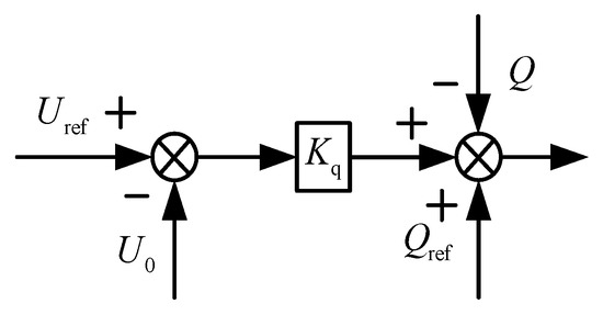
Figure 5.
Control block diagram of synchronous generator excitation regulator.
The reactive power–voltage control block diagram of the virtual synchronous generator is shown in Figure 6. The terminal voltage command value generated by the excitation regulator is input into the stator electrical equation, and the current command value is generated combined with the active power–frequency adjustment loop. The generated current command value is used as the set value of the outer current loop. The control principle block diagram of the virtual synchronous generator is shown in Figure 7.
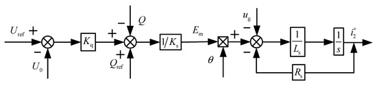
Figure 6.
Block diagram of reactive power–voltage loop structure.

Figure 7.
Control principle block diagram of virtual synchronous generator.
3. Small-Signal Modeling Analysis and Parameter Optimization Design of Virtual Synchronizer
3.1. Modeling Analysis of Virtual Synchronizer Response to Grid Frequency Fluctuations
The rotor mechanical equation of motion [25] can be expressed as:
Then,
where is the damping coefficient, is the rotational inertia, is the mechanical angular velocity, is the electrical angular velocity, is the excitation electric potential phase angle, is the mechanical power, and is the electromagnetic power.
We can combine (3) with (4) as follows:
When the system is in the initial steady state, the rated active power and rated reactive power are set to and , respectively.
When the system is in the steady state , the small disturbances , , , , , , and are added at this time, and the new state variables are:
where is the inverter’s angular frequency, is the grid’s angular frequency, is the power angle, is the terminal voltage, is the grid voltage, is the active output, and is the reactive power output.
We can combine (5) with (6):
According to (7), the small-signal model in the s-domain can be drawn, as shown in Figure 8.

Figure 8.
Small-signal modeling in response to changes in grid frequency.
The simplified active disturbance and reactive disturbance equations are expressed as
In (8):
where represents the transfer function of grid frequency fluctuation and inverter’s active output; represents the transfer function of the grid voltage fluctuation to the active output of the inverter; represents the transfer function of the grid frequency fluctuation to the inverter’s reactive output; and represents the transfer function of the grid voltage fluctuation to the reactive output of the inverter.
When the system is running stably, the value of is very small, which can be approximated as , . Through simplification, can be expressed as:
The characteristic roots of (9) are expressed as
According to (9), the natural angular frequency, damping ratio, and the amount of overshoot are expressed as:
In (11), the system frequency is mainly affected by the rotational inertia and the grid impedance . In (12), the damping effect of the system is mainly influenced by the rotational inertia , the damping coefficient , and the grid impedance . Since and are located within the root sign, the degree of influence on the damping is less than . In (13), the system overshoot is also influenced by the rotational inertia , the damping coefficient , and the grid impedance . Since is a quadratic term, its influence on the overshoot is greater than and .
3.2. Modeling Analysis of Response to Active Power Command Fluctuation
When the system is in the steady state, the rated active power and rated reactive power are set to and , respectively. When the system is in the steady state , the small disturbances , , , , , , and are added at this time, and the new state variables are
Combining (5) and (14), leaving only the first-order terms and eliminating , , , and , the expression in the s domain is:
The small-signal model can be drawn from (15), as shown in Figure 9.
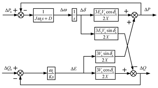
Figure 9.
Small-signal modeling in response to changes in active command values.
Additionally, after eliminating the three intermediate variables, , , and , the simplified active disturbance and reactive disturbance equations can be expressed as
Reactive disturbance equations can be expressed as
In (17):
where represents the transfer function of active command fluctuation and inverter’s active output; represents the transfer function of the reactive power command fluctuation to the active output of the inverter; represents the transfer function of the active power command fluctuation to the reactive power output of the inverter; and represents the transfer function of the reactive power command fluctuation to inverter’s reactive power output.
The control variable method is used to study the effects of rotational inertia J and damping coefficient D on the dynamic stability of the system. When the rotational inertia J = 0.002, rotational inertia J = 0.1, the root trajectory of damping coefficient D is shown in Figure 10. When the damping coefficient D is small, the system is in an unstable region. As the damping coefficient D increases, the system gradually transitions from the unstable state to the stable state. When the system starts to enter the stable state, the system is in an underdamped state with good dynamic response speed. With the continuous increase in the damping coefficient, the system is in the overdamped state, the power-dynamic waveform does not have overshoot, and the dynamic adjustment time of the system increases.
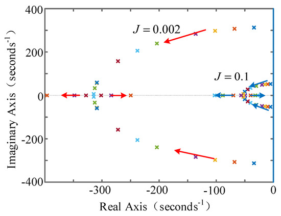
Figure 10.
Root-trajectory diagram of damping coefficient and rotational inertia.
As the rotational inertia J increases, the overshoot of the power dynamic waveform increases, weakening the effect of the damping coefficient and seriously threatening the dynamic stability and dynamic response speed of the system. The rotational inertia J and the damping coefficient D also affect the speed and amount of change of the rising and falling edges of the power waveform during the dynamic process.
With the increase in rotational inertia J, the regulation time of the system dynamic process increases, the overshoot increases, and the damping effect is weakened, while the rate of change of active power decreases, and the simulation diagram is shown in Figure 11. As the damping coefficient D increases, the overshoot of active power decreases, the dynamic adjustment time increases, and the rate of change of active power decreases. The corresponding simulation waveform is shown in Figure 12.
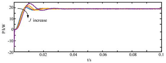
Figure 11.
Simulation of rotational inertia affecting system’s active output performance.
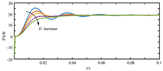
Figure 12.
Simulation of damping coefficient affecting system’s active output performance.
It can be seen from Figure 13 that the grid impedance increases. The overall performance of the system means that the dynamic response speed of the system and the overshoot of the system are reduced, and its effect is consistent when increasing the damping coefficient.

Figure 13.
Simulation of grid impedance affecting system’s active output performance in weak grid.
Equation (12) can also be expressed as:
In this paper, the engineering damping ratio , which is commonly used in actual engineering, is selected. As shown in Figure 14, when the source-side power changes suddenly from 19 kW to 29 kW, maintaining the same damping coefficient of 6.55, the overshoot of the active power under the strong grid is about 9.4%, and the overshoot of the system will disappear under the weak grid. Under the same grid impedance of 3 mH and reducing the damping coefficient to 3.55, the time for the system to reach stability changes from 0.35 s to 0.25 s. This shows that when the damping coefficient remains unchanged, increasing the grid impedance will cause the system overshoot to disappear, making the dynamic response speed slower. When the damping coefficient is reduced, the dynamic response speed of the system can be effectively improved, and the slow dynamic adjustment speed of the system can be improved. In the case of a weak grid, the uncertainty of new energy generation and nonlinear electrical equipment makes the grid-equivalent impedance of the system change in a relatively wide range. The passive detection method of grid impedance can be used to measure the grid-impedance value in real time using the small disturbance of the system itself and can then be combined with (18) to achieve the effect of online dynamic adjustment of the damping coefficient, ensuring the safety and stability of the system and attaining a faster response speed.
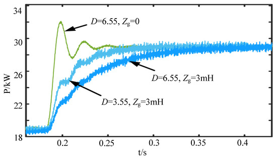
Figure 14.
Diagram of dynamic adjustment of damping coefficient.
It can be seen from Figure 14 that reducing the damping coefficient can improve the influence of grid impedance on the dynamic performance of the system under a weak grid, which verifies the theoretical analysis.
4. Simulation and Experimental Verification
4.1. Simulation Verification
The simulation platform was built in Matlab/Simulink, and the test platform was built in the laboratory. The main simulation parameters are shown in Table 1.

Table 1.
Simulation platform parameters.
As shown in Figure 15, the system operates in the initial steady state at 0~0.2 s, and the active power command increases from 19 kW to 29 kW at 0.2 s. As the inverter output active power increases, the inverter output frequency also produces a positive fluctuation, and the steady-state value is maintained at 50 Hz, always keeping the same frequency as the grid, while the inverter output current also increases. The is reduced from 29 kW to 19 kW at 0.4 s, effectively simulating the rotor characteristics of a synchronous generator. The dynamic response relationship between the active output of the inverter and the active command value is verified.
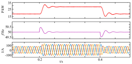
Figure 15.
Simulation diagram of active command value adjustment.
Keeping the active command value and the grid voltage value unchanged, the grid frequency of the initial state is the rated frequency of 50 Hz, and the simulation diagram is shown in Figure 16. The grid frequency decreases from 50 Hz to 49.5 Hz at 0.2 s. The grid frequency increases from 49.5 Hz to 50 Hz at 0.4 s. The dynamic process of the simulated waveform is in accordance with the active power–frequency control principle of the synchronous generator, and the output frequency of the inverter is always synchronous with the grid frequency.
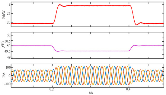
Figure 16.
Simulation diagram when the grid frequency fluctuates.
In summary, when the grid frequency and grid voltage of the virtual synchronizer system are kept constant, the system output active power can follow the commanded value of active power; when the commanded value of active power and grid voltage are kept constant, the system output frequency can follow the change of grid frequency.
4.2. Experimental Verification
As shown in Figure 17a, the main circuit part of the experimental platform includes devices such as DC-side voltage regulator capacitors, switching tubes, filter inductors, and filter capacitors.
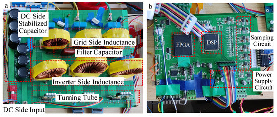
Figure 17.
Experimental platform circuit. (a) The main circuit; (b) The control circuit.
Figure 17b shows the control circuit part of the test platform, which is mainly composed of the DSP of the TMS320F28335 model and the FPGA of the EP3C25Q240C8N model.
The waveform diagrams of the output current, output active power, and grid frequency of the grid-connected inverter before and after changes are shown in Figure 18 and Figure 19. It can be seen in Figure 18 that when the grid frequency is increased from 50 Hz to 50.05 Hz, the output current of the grid-connected inverter decreases, while the active output decreases; in Figure 19, it can be seen that when the grid frequency is reduced from 50 Hz to 49.95 Hz, the output current of the grid-connected inverter increases, and the active output increases, which verifies the theoretical analysis of this article.
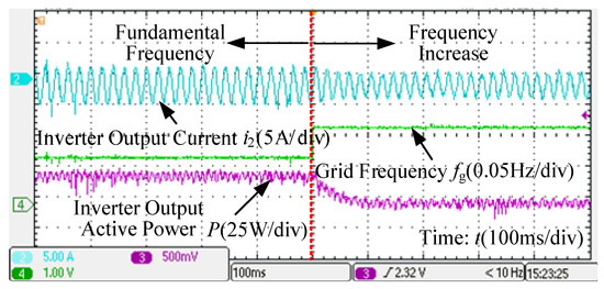
Figure 18.
Inverter output current and output active power waveform when the grid frequency is reduced.
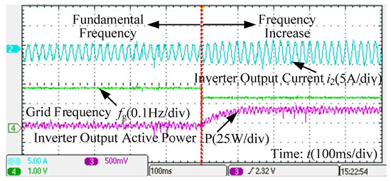
Figure 19.
Inverter output current and output active power waveform when the grid frequency rises.
According to the theoretical analysis in Section 3, the grid impedance will also affect the dynamic response speed of the system. The addition of the grid impedance can also increase the damping coefficient. Therefore, in a weak grid system, dynamically adjusting the damping coefficient can be used to adapt to the fluctuation of the grid impedance and ensure the dynamic response speed.
Figure 20 shows the output active power and output frequency of the inverter when the damping coefficient D = 8.35 under a strong grid, and Figure 21 shows the output active power and output of the inverter when the grid impedance Zg = 6 mH and the damping coefficient D = 8.35 under a weak grid. It can be seen from Figure 20 and Figure 21 that the dynamic response speed of the system slows down as the grid impedance increases. It can be seen from Figure 21 and Figure 22 that the dynamic response speed of the system can be improved by reducing the damping. The feasibility of the control method is verified.
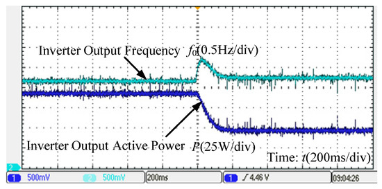
Figure 20.
The output active power and frequency of the inverter when the damping coefficient D = 8.35 in a strong grid.
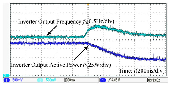
Figure 21.
The output active power and frequency of the inverter when the damping coefficient D = 8.35 in a weak grid.
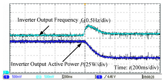
Figure 22.
The output active power and frequency of the inverter when the damping coefficient D = 5.67 in a weak grid.
5. Conclusions
With the large-scale integration of renewables in modern power systems, power-electronic equipment represented by virtual synchronous generators is becoming increasingly used in power systems. In this paper, a current-source VSG is used to achieve grid-connected operation of new energy sources. Combined with weak grid conditions, the parameters of the VSG were analyzed and designed in a detailed, systematic, and theoretical way to solve the dynamic stability problem of the grid-connected inverter under small disturbances.
Considering the impedance characteristics of the weak grid, the parameters of the VSG were analyzed and designed in detail to solve the new dynamic stability problem of the grid-connected inverter under small disturbances at the source side and grid side.
First, the mathematical model of VSG was established. The active power–frequency and reactive power–voltage characteristics of the generator were analyzed.
Then, a small signal model was established under a strong grid, and the influence of grid-side frequency fluctuation and source-side power fluctuation on the dynamic performance of the inverter was discussed. Based on the model analysis and parameter optimization, the design method in this paper realized the effective control of the grid-connected system under the input-fluctuation condition.
Finally, combined with the new characteristics of weak grid-impedance change, the influence of VSG control parameters and grid impedance on the dynamic response performance of the system was explored through root locus and simulation. Through theoretical analysis and simulation comparison, the VSG control parameters designed under the strong grid affected the transient process and stability of the power system under a weak grid. This paper shows how to optimize the control parameter design according to the change of grid impedance, which can improve the dynamic stability and dynamic response speed of the system.
At the same time, system experiments were completed in this paper, including experiments under the conditions of source-side power fluctuation, grid-side frequency fluctuation, and impedance fluctuation. The experimental results verify the correctness and feasibility of the improved method.
Based on the research of this paper, the high adaptability of VSG to new energy/power-generation systems is improved.
Author Contributions
Design of model, Y.L. and J.C.; analysis of parameters, X.Z. (Xudong Zhang) and X.Z. (Xiaojun Zhao); establishment of small-signal model, Y.L., J.C. and X.W.; analysis of simulation results, X.W., X.Z. (Xudong Zhang) and X.Z. (Xiaojun Zhao); optimization of parameters design methods, Y.L. and J.C.; verification of experiment, Y.L., J.C. and X.Z. (Xiaojun Zhao); analysis of experimental results, X.W., X.Z. (Xudong Zhang) and X.Z. (Xiaojun Zhao); editing of the article, Y.L., J.C. and X.Z. (Xudong Zhang). All authors have read and agreed to the published version of the manuscript.
Funding
This research was funded by the National Natural Science Foundation of China, grant numbers 52077191 and 62003297.
Data Availability Statement
Not applicable.
Acknowledgments
Special thanks to all members of the Department of Electric and Electronic Engineering of Shi Jia Zhuang University of Applied Technology and the Key Lab of Power Electronics for Energy Conservation and Motor Drive of Hebei Province.
Conflicts of Interest
The authors declare no conflict of interest.
References
- Lv, Z.P.; Sheng, W.X.; Zhong, Q.C.; Liu, H.; Zeng, Z.; Yang, L.; Liu, L. Virtual synchronous generator and its applications in micro-grid. Proc. CSEE 2014, 34, 2591–2603. [Google Scholar]
- Liu, F.; Wang, M.; Xie, Z.; Wang, F.; Deng, J.; Zhang, X. VSG control and parameters design based on virtual synchronous generator. In Proceedings of the 2018 International Power Electronics Conference, Niigata, Japan, 20–24 May 2018; pp. 2992–2996. [Google Scholar]
- Yan, X.W.; Liu, Z.N.; Zhang, B.; Lü, Z.; Su, X.; Xu, H.; Ren, Y. Small-signal stability analysis of parallel inverters with synchronous generator characteristics. Power Syst. Technol. 2016, 40, 910–917. [Google Scholar]
- Du, W.; Jiang, Q.R.; Chen, J.R. Frequency control strategy of distributed generations based on virtual inertia in a microgrid. Autom. Electr. Power Syst. 2011, 35, 26–36. [Google Scholar]
- Meng, J.H.; Wang, Y.; Shi, X.C.; Fu, C.; Li, P. Control strategy and parameter analysis of distributed inverters based on VSG. Trans. China Electrotech. Soc. 2014, 29, 1–10. [Google Scholar]
- Toshinobu, S.; Yushi, M.; Toshifumi, I. Oscillation damping of a distributed generator using a virtual synchronous generator. IEEE Trans. Power Deliv. 2014, 29, 668–676. [Google Scholar]
- Wei, Y.L.; Zhang, H.; Song, Q. Contrlo strategy for parallel-operated virtual synchronous generators. In Proceedings of the 2016 IEEE 8th International Power Electronics and Motion Control Conference, Hefei, China, 22–26 May 2016; pp. 16–22. [Google Scholar]
- Tao, L.; Cheng, J.Z.; Wang, W.X.; Gong, J.; Sun, J. Methods of parameter design and optimization in virtual synchronous generator technology. Power Syst. Prot. Control 2018, 46, 128–135. [Google Scholar]
- Wu, H.; Ruan, X.B.; Yang, D.S.; Chen, X.; Zhong, Q.; Lu, Z.P. Modeling of the power loop and parameter design of virtual synchronous generators. Proc. CSEE 2015, 35, 6508–6518. [Google Scholar]
- Wu, H.; Ruan, X.B.; Yang, D.S.; Chen, X.; Zhao, W.; Lv, Z.; Zhong, Q.-C. Small-signal modeling and parameters design for virtual synchronous generators. IEEE Trans. Ind. Electron. 2016, 63, 4292–4303. [Google Scholar] [CrossRef]
- Wu, M.; Lv, Z.P.; Qin, L.; Song, Z.H.; Sun, L.J.; Zhao, T.; Xu, J.; Gao, J. Robust control parameter design for virtual synchronous generator under variable operation conditions of grid. Power Syst. Technol. 2019, 43, 3743–3751. [Google Scholar]
- Wang, L.; Ju, Y.T.; Wu, W.C.; Chen, X. Optimal design of inertia and damping parameters of virtual synchronous microgrid for improving frequency stability. Proc. CSEE 2021, 41, 4479–4489. [Google Scholar]
- Huang, H.; Wang, L.; Wei, Y.L.; Zhao, J.R.; Xiao, F.; Ma, B.L.; Yang, X.R. Research on the virtual synchronous generator in microgrid. Electr. Drive 2019, 49, 45–50. [Google Scholar]
- Huo, X.X.; Huang, X.; Wang, K.Y.; Yan, J.J.; Xu, K.; Yao, C.; Chen, P.Y. Research on frequency stability control for micro-grid based on virtual synchronous generator. Mod. Electr. Power 2019, 36, 45–52. [Google Scholar]
- Yang, Y.; Mei, F.; Zhang, C.Y.; Miao, H.; Chen, H.; Zheng, J. Coordinated adaptive control strategy of rotational inertia and damping coefficient for virtual synchronous generator. Electr. Power Autom. Equip. 2019, 39, 125–131. [Google Scholar]
- Deng, P.; Yang, P.H. Research on frequency optimal regulation of hybrid energy storage virtual synchronous machine. J. Power Supply 2022, 8, 1–13. [Google Scholar]
- Yan, X.W.; Zhang, W.C.; Cui, S.; Huang, H.Y.; Li, T.C. Frequency response characteristics and adaptive parameter tuning of voltage-sourced converters under VSG control. Trans. China Electrotech. Soc. 2021, 36, 241–254. [Google Scholar]
- Zou, P.G.; Meng, J.H.; Wang, Y.; Lei, X. Influence analysis of the main control parameters in FVSG on the frequency stability of the system. High Volt. Eng. 2018, 44, 1135–1342. [Google Scholar]
- Sheng, W.X.; Lu, Z.P.; Cui, J.; Liu, H.T. Calculation and parameter analysis of virtual synchronous machine operation area. Power Grid Technol. 2019, 43, 1557–1565. [Google Scholar]
- Li, J.C. Design and Application of Modern Synchronous Generator Excitation System; China Electric Power Press: Beijing, China, 2009. [Google Scholar]
- He, Y.Z.; Wen, Z.Y. Power System Analysis; Huazhong University of Science and Technology Press: Wuhan, China, 2009. [Google Scholar]
- Meng, J.H.; Shi, X.C.; Wang, Y.; Fu, C.; Li, P. Study on control strategy of Der inverter for improving frequency stability of microgrid. J. Electr. Technol. 2015, 30, 70–79. [Google Scholar]
- Erickson, R.W.; Maksimovie, D. Fundamentals of Power Electronics; Kluwer Academic Publishers: Alphen aan den Rijn, The Netherlands, 2010. [Google Scholar]
- Gao, J.; Qin, L. Input impedance modeling and stability analysis of virtual synchronous generator. Power Grid Technol. 2021, 45, 578–588. [Google Scholar]
- Kunder, P. Power system stability and control. IEEE Trans. Power Electron. 2007, 7, 103. [Google Scholar]
Publisher’s Note: MDPI stays neutral with regard to jurisdictional claims in published maps and institutional affiliations. |
© 2022 by the authors. Licensee MDPI, Basel, Switzerland. This article is an open access article distributed under the terms and conditions of the Creative Commons Attribution (CC BY) license (https://creativecommons.org/licenses/by/4.0/).