The Characterization of the Electric Double-Layer Capacitor (EDLC) Using Python/MATLAB/Simulink (PMS)-Hybrid Model

Abstract

This paper investigates the characterization of an electric double-layer capacitor (EDLC). In this study, the 300 F and 400 F EDLC supercapacitors are connected in a circuit in a laboratory experiment to produce their charge/discharge profiles at a constant current. The acquired charge/discharge profiles were used to determine the mathematical parameters of the EDLCs using the “Faranda model”, or “two-branch model”, of the EDLC. The parameters extracted from the equivalent circuit model were then used as inputs to a designed Python/MATLAB/Simulink (PMS)-hybrid model of an EDLC. This was simulated to obtain charge/discharge profiles. The resulting experimental- and simulated-charge/discharge profiles of the EDLCs were compared with each other, by superimposing their profiles to determine the accuracy of the PMS model. The PMS model was found to be very accurate. The innovation of this work lies in modeling a supercapacitor, mostly in the Python programming language in combination with a MATLAB/Simulink model. The experimental-charge/discharge profiles obtained were used to calculate the equivalent circuit resistance (ESR) and the capacitance of the EDLCs, which were compared with the existing datasheet values of the EDLCs. The characterization of the EDLC supercapacitor was done to derive a flexible PMS model of the EDLC, which can be used in a microgrid hybrid energy-storage system (HESS) to show the potential of the EDLC in improving battery lifespan.

1. Introduction

The electric double-layer capacitor is a type of energy-storage device (ESD) [1]. Energy-storage devices are used to store energy in electrical and electronic applications. The most common ESDs are conventional capacitors and batteries. Drawbacks of batteries include short life span, low discharge/charge cycles, and very low power density. Conventional capacitors have a low energy density. This has necessitated the development of a third ESD, the electric double-layer capacitor (EDLC) supercapacitor, which occupies a middle ground between the ESDs. The EDLC takes some of the characteristics of the conventional capacitor, such as high-power density and a high charge/discharge cycle, while adding a better energy density. These characteristics have it made it very useful in industries that require repeated rapid release of stored energy, such as hybrid cars [2,3,4] and microgrid hybrid energy-storage systems (HESS) [2].

EDLCs have found very useful application, especially in microgrid hybrid energy-storage systems, where they help in prolonging battery lifespan by reducing stress on the battery due to excessive power fluctuations. Table 1 below shows comparisons between different types of ESDs.

Table 1. EDLC comparison with other ESDs [3,5].

Parameters	Lead–Acid Battery	Lithium-Ion Battery	EDLC
Specific energy density (Wh/kg)	10–100	150–200	1–10
Specific power density (W/kg)	<1000	<2000	<10,000
Cycle life	1000	5000	>500,000
Charge/discharge efficiency	70–85%	99%	85–98%
Fast-charge time	1–5 h	0.5–3 h	0.3–30 s
Discharge time	0.3–3 h	0.3–3 h	0.3–30 s
Calendar life (year)	5–15	10–20	20

This research will look at the Python/MATLAB/Simulink (PMS)-hybrid mathematical model of the EDLC, derived from the equivalent experimental circuit, with the goal of characterizing our own EDLCs.

2. Literature Review

In paper [4], the authors proposed a new EDLC-equivalent model, called the “two-branch model” or sometimes called the “Faranda model”. This model, although slightly different from other models, makes the identification of equivalent circuit parameters (coefficients) much easier. Experimental tests were conducted on two samples of EDLCs, and parameters were successfully extracted from it.

Another way of EDLC characterization was proposed in article [6]. Here, the authors noted the deficiencies of the simple resistor capacitor (RC)-equivalent circuit and went on to suggest a new “three-branch parallel model”, with one of the branches incorporating a voltage-dependent capacitor. Simulated and experimental results were then compared with the datasheet values, and the model was proven correct.

The effect of heat on the characterization was studied [7]. Here, the authors investigated the thermal modeling of the EDLC. A model was proposed and tested, with the experimental and simulated results in agreement. Another piece of research [2] described how to simulate a mathematical model for both the battery and EDLC in MATLAB/Simulink, to be incorporated into a PV-microgrid system. The same principal was applied in [8], to investigate the effect of an EDLC in energy-storage systems. The simulated results and practical results were found to correlate. In [9], a voltage-current equation was used to propose an equivalent circuit for the EDLC. The authors further provided an experimental method to derive the parameters of the EDLC. These were then used to simulate the model in MATLAB/Simulink. Simulated values of the ESR and capacitance were compared with those in the datasheet.

Different methods on how to extract the parameters of the EDLC were investigated in [10]. The authors set up different laboratory experiments to obtain the charge/discharge profiles of the EDLC at a constant current. Parameters of two 15 V, 52 F EDLCs were then extracted experimentally and discussed. The authors in [11] investigated the different types of supercapacitor models that have been proposed. They concluded that, while many models exist, each one has its own advantages and disadvantages depending on the application. Similar research was conducted in the following referenced articles [5,11,12].

3. Theory of the EDLC

3.1. Structure

The EDLC is a type of supercapacitor (SC). There are three types, namely EDLC, pseudo, and hybrid SCs. The EDLC consists of two electrodes separated by a membrane, called “a separator”. Both the electrodes and the separator are immersed in a liquid-like solution called an electrolyte. The electrodes of the EDLC are normally made of a porous carbon material, which increases their surface area and, thus, gives them the ability to obtain very high capacitance. The electrodes can also be made from other materials such as graphene and metal oxides.

The maximum voltage across one cell of the EDLC is imitated to the specific maximum voltage of the specific supercapacitor, due to the breaking potential of the electrolyte. To achieve higher voltages and capacitance, multiple EDLC cells are connected in series or parallel depending on the need.

3.2. Equivalent Circuit Model

The EDLC can be represented by a very basic equivalent resistance–capacitance (RC) circuit, as shown in Figure 1 below. It consists of a series resistor that represents the equivalent series resistance (ESR), the capacitor (C), and the leakage-current’s equivalent parallel resistor (EPR) [11]. This representation, while widely used and sufficient for most basic simulation, does not take into account the nonlinear behavior of the EDLC during charge/discharge cycles.

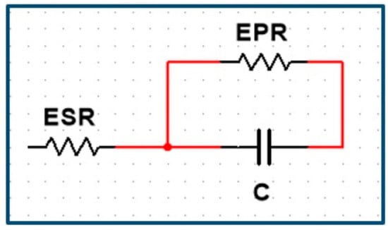
Figure 1. Basic RC model [11].

The deficiency of the basic RC model necessitated the development of other models to obtain more accurate simulations. One of those is the three-branch model, often called the Zubieta model [6,12], which consists of three parallel resistance–capacitance branches with three time constants, to cater to the different time behavior of the EDLC during charging and discharging. It also contains a voltage-dependent capacitor in the immediate branch, with a value that is dependent on the voltage.

A model very similar to the Zubieta model is the two-branch model or the Faranda model [4], as shown in Figure 2. The Faranda model consists of two instead of three resistance–capacitance branches. For this study, we will use the Faranda model as our electrical-equivalent circuit for the EDLC.

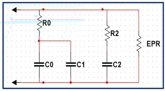
Figure 2. Two-branch model or Faranda model [4].

3.3. Mathematical Equations of the “Two-Branch Model”

The mathematical equations emanating from the two-branch electrical-equivalent circuit of the EDLC described in [2] consist of Equations (1)–(4) and represent all the branches of the “two-port”, as an equivalent circuit model.

At any one point in time, the voltage $V_{sc}$ across the EDLC cell is represented by [2]:

$$V_{SC}=N_S\left(V_1+R_1 \left(\frac{I_{SC}}{N_P}\right)\right)$$

(1)

where $N_s$ is the number of SC cells in series, $N_p$ is the number of cells in parallel, $I_{sc}$ [2] is the current of the supercapacitor (SC) module, and $V_1$ is the voltage across the capacitors in the first branch of the equivalent circuit model.

The voltage and charge across the capacitor $C_1$ in the first branch are calculated using Equations (2) and (3), respectively, as shown below [2].

$$V_1=\frac{-C_0+\sqrt{C_0{}^2+2C_v{Q}_1}}{C_v}$$

(2)

$$Q_1=C_0{V}_1+\frac{1}{2}{C}_v{V}_1{}^2$$

(3)

with $Q_1$ being the total charge accumulated across $C_1$, $C_v$ is the voltage dependent capacitance and $C_0$ is the value of the capacitor in the first resistance–capacitance line [2].

The voltage and charge of capacitor $C_2$ in the second branch are calculated equally, using Equations (4) and (5), from [2,9] respectively.

$$V_2=\frac{1}{C_2}{\displaystyle \int }{i}_2 dt=\frac{1}{C_2}{\displaystyle \int }(V_1-V_2)/R_2 dt$$

(4)

where $C_2$ and $R_2$ are the values of the capacitance and resistance of the second-branch-equivalent circuit, $V_2$ and $I_2$ are the voltage and current in the second branch [9].

$$Q_2=V_2{C}_2$$

(5)

with $Q_2$ being the total charge, $V_2$ is the voltage in the branch and $C_2$ is the capacitance in the branch.

4. Materials and Methods

The research was conducted on two Eaton Bussmann EDLCs, with a datasheet summary that is shown in Table 2 below.

Table 2. EDLCs datasheet values.

Capacitance	Max Voltage	ESR
400 F	2.7 V	3.2 mΩ
300 F	2.7 V	6 mΩ

The characterization process used is described as follows.

4.1. Two-Branch-Model Parameter Extraction Using Circuit Experiments

An experiment was set up in the laboratory to acquire the charge/discharge profiles of the EDLCs, with charging done at a constant current of 2 A until the EDLCs reached their maximum voltages of 2.7 V. Discharging was done by removing the current and adding a load. Henceforth, using the charging profile derived, the parameters were extracted and used as an input to the “two-branch model” designed in the Python/MATLAB/Simulink (PMS) model. The mathematical equations used in the Python/MATLAB/Simulink (PMS)-hybrid model are described as follows.

The first branch consists of $R_0$ and $C_1$ [4], which cater to the immediate behavior of the EDLC during charging/discharging. To find the value of the resistance $R_0$, the change in voltage right at the beginning of the charging profile is divided by the total constant current, as shown in (6) [4]

$$R_0=\frac{∆V}{I_C}$$

(6)

with ∆V being the change in voltage, $I_c$ is the charging current.

The capacitance $C_1$ consists of a capacitor $C_o$ and a voltage-dependent capacitor $k_v$. These are calculated by taking two points on the charge profile, $P_1$ ($t_1$, $v_1$) and $P_2$ ($t_2$, $v_2$) [4] and substituting the values in (7) and (8). Previous experiments [4] have shown that it is good practice to chose $P_1$ and $P_2$ at 1.2 V and 2.3 V, respectively, for a 2.7 V supercapacitor [4].

$$C_0=\left(\frac{t_1}{V_1}-\frac{V_1·t_2-t_1·V_2}{V_2{}^2-V_1·V_2}\right)·I_C$$

(7)

The value of $k_v$ which is the voltage dependent capacitance is derived using Equation (8) [4]:

$$k_v=2.\left(\frac{V_1.t_2-t_1.V_2}{V_1{V}_2{}^2-V_1{}^2.V_2}\right)·I_C$$

(8)

The second branch of the “two-branch model” [3,4] is calculated using (9), consisting of $R_2$ and $C_2$, which cater for the long-term behavior of the EDLC during the charging/discharging process [4].

$${\tau }_2=R_2{C}_2$$

(9)

An estimated value for time constant ${\tau }_2$ is taken around 240 s [4], based on the charge profile of the supercapacitors used. $C_2$ is calculated using Equation (10) [4].

$$Q_{tot}=I_C.T_C=C_2.V_{2f}+\left(C_0+\frac{k_v}{2}.V_{2f}\right).V_{2f}$$

(10)

where $Q_{tot}$ is the total EDLC accumulated charge, $I_C$ is the charging current, $V_{2f}$ is measured at three times ${\tau }_2$ [4], and $T_C$ is the time constant. After calculating the value of $C_2$, Equation (9) is used to acquire the value of $R_2$.

4.2. Python/MATLAB/Simulink (PMS)-Hybrid Model

After acquiring the parameters’ values for the supercapacitors of the two-branch equivalent model from the experimental laboratory circuit, an algorithm to model the EDLC was developed, which was the Python/MATLAB/Simulink (PMS)-hybrid model, using the same standard mathematical equations as a supercapacitor. The parameters from the experimental wired setup were fed into the PMS model. The algorithm designed in the Python/MATLAB/Simulink (PMS) model was used to derive a simulation model for the EDLCs. The PMS model was then executed to acquire a charge profile for the supercapacitor. The key to the PMS model was in solving the differential mathematical equations that represent the supercapacitor using Python programming. A comparison was made between the experimental data’s charge/discharge curves and the PMS data’s charge/discharge curves from the supercapacitors, to determine the accuracy of the model and its underlining algorithm.

4.3. Equivalent-Series Resistance (ESR) and Capacitance Calculation

The equivalent-series resistance (ESR) and capacitance for the 300 F and 400 F EDLCs were calculated using the discharge profiles acquired both experimentally and by simulation, which were then compared with datasheet values.

The ESR is measured at the beginning of the discharge profile using (11), with $∆V$ being the immediate drop in voltage observed on the discharge profile, when a load is connected drawing current $∆I$ [10].

$$ESR=\frac{∆V}{∆I}$$

(11)

whereas the capacitance is determined by (12) and (13), using the linear part of the discharge profile [10].

$$C=\frac{∆Q}{∆V}$$

(12)

where, ∆Q the change in total charge, and ∆V is the change in voltage. The change $∆Q$ and $∆V$ are calculated by taking two time instants, $t_1$ and $t_2$, in the linear part of the charge/discharge curve [10].

$$C=\frac{{{\displaystyle \int }}_{t_1}^{t_2}i \left(t\right) dt}{v_1-v_2}$$

(13)

with $V_1$ the voltage at $t_1$, $V_2$ is the voltage at $t_2$ and $i$ is the charge/discharge current.

5. Experimental

5.1. Parameter-Acquisition Procedure and Experimental Setup

The experimental set up in the laboratory that is used to obtain the EDLC’s charge/discharge profile is shown in Figure 3. This charge/discharge profile is used to characterize the supercapacitors. It consists of a Tektronix four-channel digital-storage oscilloscope, with a bandwidth of 40 MHz and a sampling rate of 1 GS/s; a Delta Electronics 15 V, 10 A adjustable DC-current source, to provide the constant current to charge the EDLC during the charging process; a variable resistor to act as a load during the discharging process; and a digital multimeter used to measure the voltage across the EDLC and the current during the charge/discharge process. The voltage data are also measured on the oscilloscope. The voltage data obtained are plotted using the “origin” software.

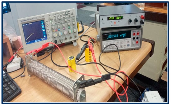
Figure 3. Experimental setup.

During the charging process, the current source was connected to the EDLC, and the load was disconnected. The EDLC was then charged at a constant current of 2 A until it reached its maximum voltage of 2.7 V. For the discharge process, the charged EDLC was disconnected from the current source and connected to the load, which is a variable potentiometer with a resistance that was adjusted to 1.35 Ω to allow the EDLC to discharge at a current of 2 A.

5.2. Python/MATLAB/Simulink (PMS) Modeling

A flowchart of the of the EDLC’s mathematical model is shown in Figure 4. It consists of the derived parameters, denoted using the color “green”, extracted from the experimental circuit. The input constant current and the output voltage are in “violet”. The circle in “yellow” represents the “feedback loop” and contains the variables $Q_1$, $Q_2$, $V_1$, and $V_2$, which are dependent on each other. With $Q_1$ being the charge on capacitor $C_1$, $Q_2$ is the charge on $C_2$. $V_1$ and $V_2$ are the voltages on the capacitances of the supercapacitor, respectively.

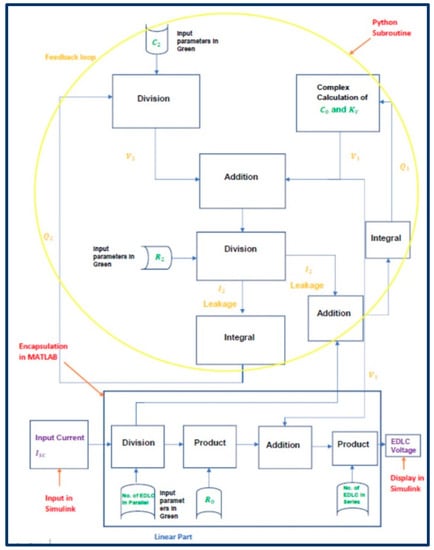
Figure 4. Python/MATLAB/Simulink (PMS) flow chart.

In the flowchart, the input current is divided by the number of EDLC cells in parallel, which in this case are set to one in the code. The result of this is fed into the feedback loop. In the feedback loop, the values for the dependent variables $Q_1$, $Q_2$, $V_1$, and $V_2$ are calculated. This feedback loop is responsible for the exponential increase in the EDLC’s voltage, when a constant current is applied.

The output of the feedback loop $V_1$ is then added and multiplied by the number of EDLC cells in the series, which in this case are also set to one, to provide an output that is the voltage across the EDLC.

This feedback loop, as well as the division and multiplication of the EDLC cells, is done using Python code; subsequently, the Python code is encapsulated into the MATLAB code in order to use the input and output functionality of Simulink to collate the data generating the PMS model. This procedure is summarized in the flow diagram shown in Figure 4 below.

To acquire the values of the variables in the feedback loop, the differential Equations (14) and (15) were solved using the code in Python [2].

$$\frac{d{Q}_1}{dt}=\frac{I_{sc}}{N_p}-\frac{V_1-V_2}{R_1}$$

(14)

$$\frac{d{Q}_2}{dt}=\frac{V_1-V_2}{R_2}$$

(15)

These differential equations show the relationship between the variables $Q_1$, $Q_2$, $V_1$ and $V_2$ and are what gives the EDLC its distinct characteristics. The code in Python takes in the parameters, which in this case are the two-branch-model-derived parameters. The differential equations are then solved using Python programming. The values of $Q_1$ and $Q_2$ at any given point in time are returned in a Python list and used to calculate the values of $V_1$ and $V_2$.

A MATLAB code is used to import the Python code into a MATLAB block function encapsulating the code and using the Simulink to display the input and output functionality.

Figure 5 below shows the Python/MATLAB/Simulink (PMS) model, consisting of the Python/MATLAB function together with the Simulink constant block for the values of the parameters, and a Simulink scope and display to show the output voltage values.

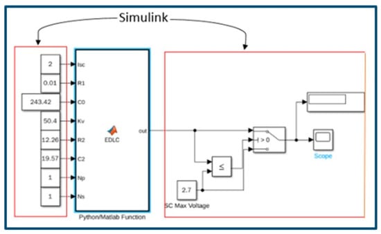
Figure 5. Python/MATLAB/Simulink (PMS) model.

6. Results

6.1. Experimental Charge/Discharge Results

The experimental-charge profile of both the 300 F and 400 F were obtained at a 2 A constant current, as shown in Figure 6. The 300 F ELDC clearly has a higher gradient curve and charges faster than the 400 F supercapacitor.

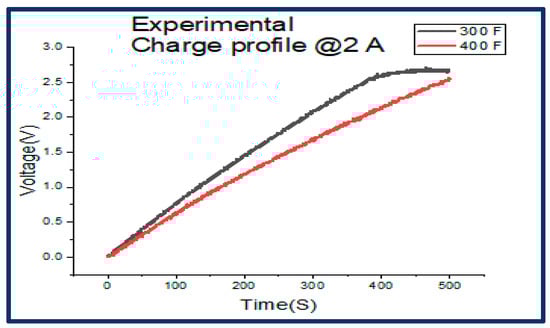
Figure 6. Experimental 300 F and 400 F charge profiles.

The charge profile and data obtained during the experiment were used to calculate the parameters/coefficients of the EDLCs two-branch-equivalent circuit. The results for the parameters are shown in Table 3 below.

Table 3. EDLC parameters.

Parameter	Eaton 300 F	Eaton 400 F
$R_1$ [Ω]	0.01	0.01
$C_0$ [F]	243.42	297.05
$k_V$ [F/V]	50.4	70.46
$R_2$ [Ω]	12.26	8.77
$C_2$ [F]	19.57	27.36

Similarly, the discharging of the EDLC was conducted at a constant current of 2 A, using a 1.35 Ω load. The discharge profiles for the two supercapacitors are captured in Figure 7.

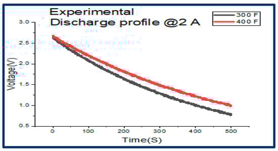
Figure 7. Experimental 300 F and 400 F discharge profile.

As expected, the 300 F EDLC discharges at a faster rate than the 400 F, which is shown by the gradient being higher. The data from the discharge profile were used to calculate the ESR and the capacitance for the respective EDLCs, the results of which are shown in Table 4.

Table 4. Results for 300 F and 400 F from the discharge profiles.

ESR and Capacitance	300 F	400 F
Load [Ω]	0.280	0.280
Current [A]	2	2
$V_1$ [Volt]	2.752	2.744
$V_2$ [Volt]	2.688	2.704
ΔV [Volt]	0.064	0.040
ESR [Ω]	0.0065	0.00408
Capacitance [F]	319 F	421 F

6.2. Simulated Results from the PMS Model

The simulated-PMS-charge/discharge profiles for both the 300 F and 400 F supercapacitors are superimposed, as can be seen in Figure 8. The simulation was done at a constant current of 2 A. The 300 F supercapacitor charges faster, as can be seen by the higher gradient in the charging profile, and it also discharges faster, as can be seen by the higher gradient in Figure 8.

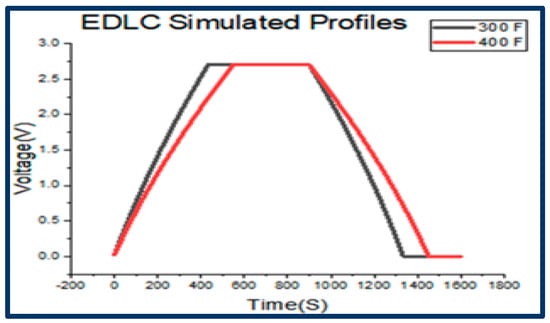
Figure 8. Simulated-PMS-charge/discharge profiles for the EDLCs.

7. Discussion

Superimpostion of Experimental-Charge/Discharge Profiles on Simulated-PMS-Charge/Discharge Profiles

The results showed similarity between the experimental and simulated-PMS-charge profiles. Figure 9 shows the charge curve for the 300 F EDLC for the experimental circuit and for the simulated-PMS model, which is superimposed. This figure shows that the two curves show a nearly perfect fit, verifying the correct extraction of the parameters from the live, experimental, wired setup, used to develop the PMS model.

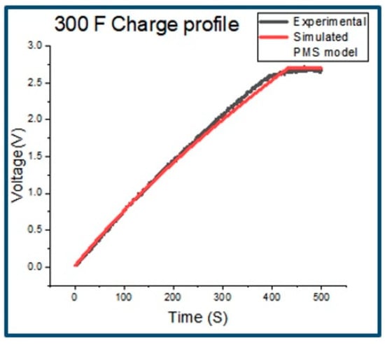
Figure 9. The 300 F EDLC superimposed experimental/PMS-charge profile.

Figure 10 shows the charge curve for the 400 F EDLC for the experimental circuit and for the simulated-PMS model, which is superimposed. This figure shows that the two curves again show a nearly perfect fit, verifying the correct extraction of the parameters from the live, experimental, wired set up, used to develop the PMS model.

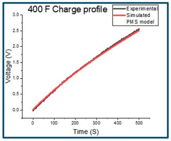
Figure 10. The 400 F EDLC superimposed experimental/PMS-charge profile.

Very noticeable is that the charge time for the two specific EDLCs, namely the 300 F and 400 F EDLCs, is quite large, making the EDLC very useful as a buffer between the source voltage and a battery. As a result of this, the battery is partially disconnected from the source voltage by the supercapacitor and can encounter less stress [13,14] in a microgrid HESS system, thus improving battery life [15].

The two discharge profiles superimposed for the 300 F supercapacitor, that is, for the experimental circuit and for the PMS model, as shown in Figure 11, are similar and depict a nearly perfect match except for a slight deviation. This deviation arises as a result of the fact that the extracted parameters from the experimental circuit, used as inputs to the simulated-PMS model of the supercapacitors, are obtained only from the charge profiles of the experimental circuit and not from the discharge profiles of the experimental circuit. Hence, the charge profile obtained experimentally perfectly matches the simulated-PMS-charge profile. However, the discharge profile obtained experimentally does not perfectly match the simulated-PMS-discharge profile. The same analysis applies to the two discharge profiles, namely the experimental and simulated-PMS model for the 400 F supercapacitor, as shown in Figure 12.

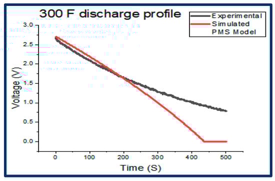
Figure 11. 300 F combined experimental/PMS-discharge profile.

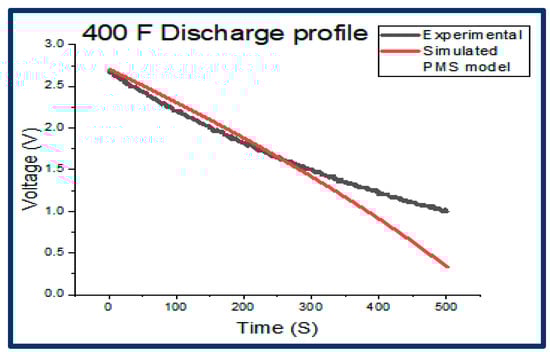
Figure 12. 400 F combined experimental/PMS-discharge profile.

The equivalent circuit parameters of the two-branch model, obtained per the procedure described in [4] for both the 300 F and 400 F Eaton Bussmann EDLCs, were found to be consistent with the similar-range datasheet EDLC values. Furthermore, the data showed that as the total capacitance of the EDLC increases, so do the values of $C_O$, $K_V$, and $C_2$, while the value of $R_2$ decreases.

The calculated ESR and capacitance of the 300 F and 400 F EDLCs showed a slight deviation from the values provided in the datasheet, as shown in Table 5 below. This might be due to factors in the laboratorial setup, such as contacts, reading meters, human error, and variations in other factors that may differ from the perfect, clean-room setups used to obtain the datasheet values.

Table 5. ESR and capacitance.

ESR and Capacitance	300 F		400 F
	ESR (mΩ)	Capacitance (Farads)	ESR	Capacitance (Farads)
Datasheet	6 mΩ	300 F	3.2 mΩ	400 F
Experimental	6.5 mΩ	319 F	4.08 mΩ	421 F

8. Conclusions

EDLC (supercapacitors) are the energy-storage devices of the future, due to their many advantages over existing energy-storage devices (ESDs) and the potential scope of their future uses. In this study, 300 F and 400 F EDLCs were characterized using the “two-branch/Faranda” method [3,4]. Experimental tests were done in the laboratory to extract equivalent circuit parameters. These parameters were then introduced into a mathematical model of the supercapacitor, which was designed in Python/MATLAB/Simulink (PMS). Subsequently, the model was simulated. The derived parameters were found to be consistent with the similar-range EDLCs in the literature. The calculated ESR and capacitance values from the experiments and simulations were found to be close to the datasheet values. Furthermore, the simulated-PMS- and experimental-charge/discharge profiles for both EDLCs were found to be almost identical in terms of the charge profiles and similar for the discharge profiles. A slight deviation occurred between the simulated-PMS model and the experimental circuit for the discharge profile. This was due to the extracted parameters from the experimental circuit coming from the charge profile only. The parameters were not obtained from the discharge profile. This study proves the accuracy of the mathematical Python/MATLAB/Simulink (PMS) model as a data representation of a supercapacitor. During the study, it was discovered that the EDLC can be modeled using a Python/MATLAB/Simulink (PMS)-hybrid model.

References

- Cultura, A.B.; Salameh, Z.M. Performance evaluation of a supercapacitor module for energy storage applications. In Proceedings of the IEEE Power & Energy Society General Meeting—Conversion & Delivery of Electrical Energy in the 21st Century, Pittsburgh, PA, USA, 20–24 July 2008; pp. 1–7. [Google Scholar] [CrossRef]
- Argyrou, M.C.; Christodoulides, P.; Marouchos, C.C.; Kalogirou, S.A. Hybrid battery-supercapacitor mathematical modeling for PV application using Matlab/Simulink. In Proceedings of the 53rd International Universities Power Engineering Conference (UPEC), Glasgow, UK, 4–7 September 2018; pp. 1–6. [Google Scholar] [CrossRef]
- Sahin, M.E. An investigation on supercapacitors applications with module designing and testing. J. Eng. Res. 2021. [Google Scholar] [CrossRef]
- Faranda, R.; Gallina, M.; Son, D.T. A new simplified model of Double-Layer Capacitors. In Proceedings of the International Conference on Clean Electrical Power, Capri, Italy, 21–23 May 2007; pp. 1–5. [Google Scholar] [CrossRef]
- Sahin, M.E.; Blaabjerg, F. A Hybrid PV-Battery/Supercapacitor System and a Basic Active Power Control Proposal in MATLAB/Simulink. Electronics 2020, 9, 129. Available online: https://www.mdpi.com/2079-9292/9/1/129 (accessed on 20 March 2022). [CrossRef] [Green Version]
- Zubieta, L.; Bonert, R. Characterization of Double-Layer Capacitors for Power Electronics Applications. IEEE Trans. Ind. Appl. 2000, 36, 199–205. [Google Scholar] [CrossRef] [Green Version]
- Gualous, H.; Louahlia, H.; Gallay, R. Supercapacitor Characterization and Thermal Modelling With Reversible and Irreversible Heat Effect. IEEE Trans. Power Electron. 2011, 26, 3402–3409. [Google Scholar] [CrossRef]
- Popoola, K. Modelling and Simulation of Supercapacitor for Energy Storage Applications. ADBU-J. Eng. Technol. (AJET) 2018, 7, 1–6. Available online: https://journals.dbuniversity.ac.in/ojs/index.php/AJET/article/view/448 (accessed on 20 March 2022).
- Sahin, M.E.; Blaabjerg, F.; Sangwongwanich, A. Modelling of Supercapacitors Based on Simplified Equivalent Circuit. CPSS Trans. Power Electron. Appl. 2021, 6, 31–39. [Google Scholar] [CrossRef]
- Gaswi, A.A.; Tennakoon, S.B. Modelling of Super Capacitor Modules and Parameter Extraction. In Proceedings of the 46th International Universities’ Power Engineering Conference, Soest, Germany, 5–8 September 2011; Available online: https://ieeexplore.ieee.org/document/6125630 (accessed on 20 March 2022).
- Kai, W.; Baosen, R.; Liwei, L.; Yuhao, L.; Hongwei, Z.; Zongqiang, S. A review of Modeling Research on Supercapacitor. In Proceedings of the Chinese Automation Congress (CAC), Jinan, China, 20–22 October 2017; pp. 5998–6001. [Google Scholar] [CrossRef]
- Negroiu, R.; Svasta, P.; Vasile, A.; Ionescu, C.; Marghescu, C. Comparison between Zubieta Model of Supercapacitors and their Real Behavior. In Proceedings of the IEEE 22nd International Symposium for Design and Technology in Electronic Packaging (SIITME), Oradea, Romania, 20–23 October 2016; pp. 196–199. [Google Scholar] [CrossRef]
- Oussama, H.; Othmane, A.; Amine, S.M.; Amine, H.M.; Abdeselem, C.; Abdelkader, A.B. Modelling and Comtrol a DC-Microgrid Based on PV and HESS Hyvrid Energy Storage System. In Proceedings of the First International Conference on Smart Grids, CIREI’2019, ENP-Oran, Algeria, 4–5 March 2019; pp. 1–5. [Google Scholar]
- Khan, S.A.; Rajkumar, R.K.; Wan, W.Y.; Syed, A. Supercapacitor-Based Hybrid Energy Harvesting for Low-Voltage System. In Supercapacitors; IntechOpen: London, UK, 2018. [Google Scholar] [CrossRef] [Green Version]
- Raman, S.R.; Cheng, K.-W.; Xue, X.-D.; Fong, Y.-C.; Cheung, S. Hybrid Energy Storage System with Vehicle Body Integrated Super-Capacitor and Li-Ion Battery: Model, Design and Implementation, for Distributed Energy Storage. Energies 2021, 14, 6553. [Google Scholar] [CrossRef]
Publisher’s Note: MDPI stays neutral with regard to jurisdictional claims in published maps and institutional affiliations. |
© 2022 by the authors. Licensee MDPI, Basel, Switzerland. This article is an open access article distributed under the terms and conditions of the Creative Commons Attribution (CC BY) license (https://creativecommons.org/licenses/by/4.0/).