Abstract
A model developed at the University of Tomsk, Russia, for high latitudes (over 55° N) is proposed and applied to the analysis and observation of the solar resource in the state of Sonora in the northwest of Mexico. This model utilizes satellite data and geographical coordinates as inputs. The objective of this research work is to provide a low-cost and reliable alternative to field meteorological stations and also to obtain a wide illustration of the distribution of solar power in the state to visualize opportunities for sustainable energy production and reduce its carbon footprint. The model is compared against real-time data from meteorological stations and satellite data, using statistical methods to scrutinize its accuracy at local latitudes (26–32° N), where a satisfactory performance was observed. An annual geographical view of available solar radiation against maximum and minimum temperatures for all the state municipalities is provided to identify the photovoltaic electricity generation potential. The outcomes are proof that the model is economically viable and could be employed by local governments to plan solar harvesting strategies. The results are generated from an open source model that allows calculating the available solar radiation over specific land areas, and the application potential for future planning of solar energy projects is evident.
1. Introduction
The potential of renewable energy in Mexico is well known due to the great variety of natural resources and climates in this country. One of these resources is solar radiation, which, according to several satellite models [1] and studies from international agencies such as National Aeronautics and Space Administration (NASA) or Global Solar Atlas (SOLARGIS), is abundant in Mexico [2,3]. A high solar potential region is presented in the northwest of the country, where Sonora state is located. An advantage of Sonora for solar power development is its proximity to the US which allows technological and economic interchange. This could prompt an international renewable network collaboration. The state is mainly a desert and presents extremely high and low temperatures during the year. In addition, the promotion of solar harvesting projects for energy production would reduce greenhouse gas emissions (GHGs) in the region, where electricity production represents the majority of the state CO2 emissions, with 12.2 million metric tons forecasted for the year 2020 [4]. This sector represented 34.5% of the total GHGs in Sonora in 2005 and maintains a tendency of growing each year, according to the Commission of Ecology and Sustainable Development of the State of Sonora (CEDES) and the Center for Climate Strategies (CCS) [4]. This fact, together with the potential of the region for solar energy, promotes the expansion of solar harvesting projects for energy production as an economic and ecological way of development and municipal energy planning. A key point to the design and installation of successful solar power projects in the region is to utilize a reliable source of data to illustrate the solar resource availability in the territory.
For many years, a national network for solar measurement has been promoted by the government and several institutions such as the World Meteorological Organization (WMO), the National Autonomous University of Mexico (UNAM), the Mexican Center of Innovation in Solar Energy (CEMIE-SOL), the National Council for Science and Technology (CONACYT), the Secretary of Energy (SENER), and the Mexican National Weather Service (SMN) [5,6]. The national network consists of meteorological stations distributed throughout the national territory, which measure solar radiation, using devices like pyranometers and pyrheliometers. These weather stations are classified into two types: automatic meteorological stations (EMAs) and synoptic meteorological stations (ESIMEs). EMAs consist of a system of electrical and mechanical sensors that automatically measure, record, and transmit weather variables (wind speed and direction, atmospheric pressure, temperature, relative humidity, solar radiation, and precipitation). These measurements are taken every ten minutes, and the records are transmitted every one to three hours to the national weather system. On the other hand, ESIMEs utilize electrical sensors that automatically measure the same weather variables as EMAs, but also visibility and temperature ten centimeters above ground level. In addition, ESIMEs create and send synoptic report records to the national meteorological system every three hours. Both types of weather stations of the SMN use Coordinated Universal Time (UTC) and cover a representative area of five kilometers [7]. The main weakness of the Mexican national weather network is the limited number of meteorological stations nationwide (less than 300) [7]. This leaves several locations in the country without coverage. Furthermore, these stations require constant monitoring and maintenance in order to obtain reliable data. This requires a constant supply of qualified experts and financial resources [8,9].
Currently, according to the SMN, there are 15 meteorological stations in the state of Sonora [7], which are not enough to cover several regions of the state for solar radiation measurement. Therefore, these stations provide a general view of the solar resource in the state, but not specific data for every point in the whole territory. The Mexican network of meteorological stations of the SMN is shown in Figure 1.
Figure 1.
Location of meteorological stations from the SMN in Mexico, highlighting the state of Sonora with a red outline [7,10].
Solar power plants require specific and reliable long-term data to know their viability of implementation and success of including them into the electric grid. Examples of parameters required to implement solar projects are temperature, measurements of solar radiation, geographical analysis, humidity, and meteorological data. This implies solar energy is a variable power source affected by climate, daily weather, and the day–night cycle. This illustrates the importance of specific data according to the geographical location of the intended solar power system [11]. An alternative to the use of meteorological stations is the use of mathematical models based on climatological and geographical data. These models offer a low-cost alternative compared to field stations. Moreover, mathematical models provide a good level of reliability and accuracy in results.
In recent decades, countries have researched and implemented mathematical models to predict solar radiation using different approaches. For example, a cloud observation-based model research in Gothenburg, Sweden [12], calculated global solar radiation based on the Oktas cloud scale. According to [12], this model can be used without any geographical restriction and no previous local radiation values are needed. However, this model presented limitations in resolution, which depends on long-term cloud observation records and a constant cloud observation system for higher resolution. Another case is the research conducted in Chad [13] calculating solar radiation of several cities located in different climatic zones in the country. In this study, models based on meteorological and astronomical parameters were used. These models are the Angstrom–Prescott model, the Allen model, and the Sabbagh model. These models were compared to data from the General Directorate of the National Meteorology of Chad to determine their performance and accuracy using a series of statistical metrics. The results obtained were discussed and evaluated to determine the model which predicts the best solar radiation for each city. Another interesting analysis is [14], which presented several solar radiation models developed for specific conditions in several countries and tested them in several cities of India. The results were then compared with local measurements of solar irradiance to determine which of the models has better performance in India.
The review presented in [9] analyzed several empirical models based on various approaches calculating global monthly solar radiation using meteorological parameters (sunlight, clouds, temperature, and other variables). These models were tested in the city of Yazd, Iran. The sunlight models, according to the statistical analysis in [9], were the most accurate to predict solar radiation in Iran. However, this approach requires sunlight records which are not always available. They concluded that other approaches like cloud-based or temperature can be used instead with acceptable accuracy. According to [9], the advantages of these approaches are inputs easily available everywhere. Other interesting research studies were presented in [15,16], where various mathematical models were compared to determine the optimal tilt angles to capture solar radiation on tilt surfaces for several locations worldwide. The performance of these models was analyzed for several latitudes and parameters to determine a tilt angle that provides the best performance for solar radiation for inclined surfaces. According to [16], the Koronakis and Liu–Jordan models were among the most accurate models to determine optimal surface inclination angles throughout the year. These studies are important for solar projects, which are searching for the best performance possible in their solar power installations.
A different approach to calculate daily solar radiation was presented by [17], where a model based on trigonometrical correlations was presented. This model was examined using statistical metrics against three existing models implemented on nine meteorological stations in China as reference data. Then, the proposed model was compared against 70 other meteorological stations in China to determine its errors and performance. According to [17], the proposed model resulted as simple, effective, and reliable to determine daily solar radiation in China. A similar research was presented by [18], where a series of new daily and monthly solar radiation models were presented. These models were examined in six cities in Iran against four existing models for several parameters to determine the accuracy of the new models using statistical metrics. Further, four extra cities in other countries were used to prove the accuracy of the new proposed models in latitudes worldwide. According to [18], the new models presented excellent results in general for all calculations. In addition, a highlight finding was that the new models presented a general better performance than the existing reference models.
A cloud cover model developed for Yakutia, Russia, was presented by [19], where solar radiation on tilt and horizontal surfaces was analyzed for production of hot water in permafrost regions in the Russian Arctic. The model utilized a five-year database of cloudiness in the city of Yakutsk. Hourly, daily, monthly, and annual radiations were calculated using the model. The results were compared against field testing measures in the region. In addition, the results obtained from the cloud cover model were analyzed for hot water production and storage using performance models for solar thermal systems. The objective was determining the cost efficiency of these systems throughout the year in Yakutia. The conclusion of [19] was that the information provided by the research in the permafrost region of Russia can be used to develop efficient thermal solar systems for reducing the carbon footprint of the region by using solar energy for water heating.
The review of cases provided in the previous paragraphs demonstrates the reliability and economic viability of mathematical models for the prediction of solar radiation worldwide. For the current inquiry, a model developed by the University of Tomsk [20] calculating solar global radiation on tilt surfaces was used as a base. This model was adapted to determine global solar radiation on a horizontal surface (ground-level solar radiation) in the state of Sonora in Mexico. This model was originally designed for high latitudes in Russia (over 55° N), hence a performance analysis at local latitudes in Sonora is required to ensure its accuracy. The main intention of the current research is to provide a wide distribution view of solar radiation in the state. This research work proposes this model as a useful tool to provide specific, low-cost, and reliable data for a wide and detailed view of solar radiation available in the state. Furthermore, it complements field measures from meteorological stations and satellite sources to guide the implementation of future solar power projects and promote the carbon footprint reduction due to electricity generation in the region.
The remainder of this paper is organized as follows. Section 2 presents the data sources utilized for calculations and for the determination of the accuracy in the model results. In addition, the criterion of the selection of field data is explained. Section 3 explains the methodology of the model and the strategies utilized to determine its performance. This section also describes a proposal of a geographic view of the results obtained from the model for later analysis and discussion. In Section 4, the results obtained are analyzed and discussed. Additionally, the utility, opportunities, and performance of the results in future solar projects are highlighted. Finally, Section 5 is the conclusion, where the main points of the research are presented. This section provides a global view of findings, key ideas, scopes, limitations, and suggestions about the current research work. In addition, a brief suggestion for future research is provided.
2. Data Sources
Two data sources were utilized in this research work to calculate the results obtained by the proposed model. Moreover, these sources were used as references to compare against the model and determine its performance and accuracy. These data resources are as follows: real-time measurements of the SMN meteorological stations taken from the Mexican National Water Commission (CONAGUA) [7], and satellite measurements from the NASA Surface Meteorology and Solar Energy (SSE) database [2].
2.1. SMN
The meteorological stations from the SMN selected were determined utilizing a selection criterion to avoid data gaps in the record and ensure proper data to analyze and compare against the model results. This criterion is based on the restrictions discussed in [8]. The selection conditions are as follows:
- Stations with less than 85% of the data available are discarded.
- Consistency in the data record; avoiding data gaps which may mean errors in measures reported by the stations. The previous fact may be due to the need for calibration of the station equipment [6] or due to shadows projected on the sensor because of obstacles that trigger a consistent daily loss of readings in data.
- A range of < 1300 W/m2 for readings in stations over 1000 m above the sea level and < 1100 W/m2 for the rest of the stations.
Meteorological stations in the Mexican network (SMN) provide data every 10 min, and a daily average of total solar radiation in W/m2 is taken. Then, monthly and yearly averages are calculated and converted to kWh/m2. A sample of 5 years (from 2015 to 2019) was analyzed to calculate mean values for monthly and yearly data for comparison.
Five meteorological stations were considered for analysis. These stations represent 33.3% of the total of fifteen stations in the state. The selected stations are described in Table 1.

Table 1.
Selected meteorological stations in Sonora (location and altitude) [7].
During the analysis and selection of the stations, some unexpected high values were found (measures of more than 1100 kWh/m2) in certain stations. This was especially so in El Pinacate, but it was selected for comparison due to its data availability.
2.2. NASA SSE Power Project
The NASA SSE Power project is an international satellite database available online which includes data from 1981 to present. This information includes meteorological and renewable resources such as measurements for solar, wind, temperature, moisture, and cloud index. This resource is reliable, and it is based on satellite observation and mathematical models for information worldwide [2,21]. The current research work utilized from this data source yearly averages (39 years) of the following parameters: all-sky solar radiation arriving at a horizontal surface, clearness index, and surface albedo.
3. Methodology
The methodology of the research is based on three phases. The first phase is the description of the mathematical model utilized. The second is the analysis of the model accuracy and performance based on statistical metrics for a case of study (Sonora), where the model is compared against real-time measurements of solar irradiance gathered from meteorological stations from the SME and the NASA SSE database. The last phase is the comparison and analysis of data obtained from the model for municipalities of Sonora, using heat maps to provide a geographical view of the solar resource distribution and viability of future solar power projects in the region.
3.1. Mathematical Model
The model is based on clustering the total radiation arriving at an inclined surface in three elements: direct, scattered, and reflected. The model inputs are surface albedo and clearness index obtained from the NASA SSE Power project database for the geographical location of interest [20]. All of these data are available using online tools such as the NASA SSE Power database [2] and Google Earth [10]. This allows the model to avoid investment in field equipment to collect solar irradiance measurements and provides great flexibility in data collection [20]. The model is explained in detail below.
Solar radiation arriving at a receiving surface depends upon factors such as geographical location (latitude and longitude), the day–night cycle, the date in the year, and the orientation of the receiving surface with respect to the Sun. These factors are called deterministic factors, and they vary yearly or daily and can be calculated by analytical formulas based on solar geometry [12,20].
According to [22], the day number () can be simplified from 365 days (full year) to 12 days to provide a representative monthly average, which presents an accurate estimation for solar radiation analysis [23]. This monthly average relationship is given in Table 2.
Table 2.
Day numbers per month according to [22,23].
The declination angle of the Sun () is the angular relationship between the solar position at solar noon and the equatorial plane, where: northwards (+) and southwards (−). This angle varies throughout the year () [24,25]. According to [15,26], it is given by the following equation:
The solar hour angle () depicts the rotation of Earth around its axis, and each hour is equal to 15°, where: solar noon = 0, morning hours (−), and afternoon hours (+) [16,27]. According to [23], it can be obtained from
where: is the time of the day in hours; is the time zone hour difference with respect to the Greenwich meridian as the origin, for Sonora = −7; is the equation of time; and is the longitude in degrees.
The equation of time () reflects the speed variation on Earth’s orbital movement throughout the year [11], and it is calculated from [23]
with determined by the equation
The incidence angle () portrays the angle between sunbeams and the normal on a receiving surface [11]. It can be obtained by
where: is the latitude given in radians; is the slope angle of the receiving surface with respect to the horizontal; and is the surface azimuth angle, illustrating the variation in the projection on a horizontal plane of the normal to the surface from the local meridian, with south-facing considered as = 0, eastwards (−), and westwards (+), () [24]. In this paper, angles and are considered 0 for this paper’s calculations, due to the studied surface being the ground itself and there being no inclination difference to consider. All the angles are considered in radians in the previous formula.
The solar zenith angle () is the angular relationship between the Sun’s rays and the vertical. For horizontal surfaces, [11]. It is given by
The solar altitude angle () is the angle between the sunbeams and the horizontal [24]. It keeps the following relation:
utilizing trigonometric relationships, the following equation can be obtained:
The solar azimuth angle () reflects the relationship between sunbeams and the horizontal plane, where east direction (−) and west (+) [11,28]. According to [23], this angle is determined by
According to [29], the hourly diffuse coefficient () is
The sunset hour angle () is taken from [11]
The hourly transparency coefficient (), according to [30], can be calculated by
where the values of and can be obtained utilizing the following formulas:
There are other factors called stochastic factors that also influence the solar radiation arriving at a receiving surface on Earth. These factors represent the state of the atmosphere and they are estimated based on an analysis of statistical models for long periods of observations and simulations. Examples of these factors are as follows: distribution of atmospheric gases, the density of particles in the air, air pressure, or cloud type at the site under study [12,20]. The clearness index () and diffusion index () are stochastic factors.
The clearness index (), according to [29], maintains the following relationship:
with taken from the NASA SSE database [2]; is the average daily extra-atmospheric insolation arriving at a horizontal surface [20,23]; and is the average daily radiation arriving at a horizontal surface [11]. They can be calculated from the following formulas:
where: is the solar constant = 1367 W/m2, representing the energy acting on a unit area per unit of time outside of the atmosphere at halfway from Earth to Sun [24]. All angles in the previous formula are in radians.
The diffusion index (), as stated by [29], keeps the relationship below:
The average daily diffuse radiation arriving at a horizontal surface is calculated from
According to [21], can be determined by a series of polynomial equations conditioned by angles ( and ), where is determined based on .
Table 3 shows the equations and conditions to determine the diffusion index . All the angles shown in Table 3 are expressed in degrees.
Table 3.
Conditional table to determine the diffusion index () [21].
The hourly total radiation arriving at a horizontal surface is divided into two components: direct and diffuse. The reflection part is not included for horizontal surfaces because there are not any angles that allow reflection between the surface and the horizontal. These components can be calculated as follows:
Total ():
Diffuse ():
Direct ():
According to [24], the hourly extra-atmospheric radiation arriving at a horizontal surface () is given by
Finally, as specified by [20,31], the total radiation arriving at an inclined surface () can be calculated by the following equation:
where: is the surface albedo obtained from the NASA SSE database, expressing the reflective capacity of the ground and varying according to different terrains (snow, sand, grass, etc.) and the seasons of the year [25]; and, as determined by [20,31], is the anisotropic index and can be obtained by the following formula:
3.2. Determination of Accuracy and Performance
The accuracy and performance of the model are determined by comparing data from several meteorological stations in Sonora. The proposed model is compared against two data sources: real-time measurements of the SMN taken from CONAGUA [7], and the NASA SSE database [2].
3.2.1. Statistical Metrics
Eight statistical metrics are proposed for the analysis and determination of the accuracy and performance of the model. These metrics are described as follows:
Mean absolute error () provides the average error magnitude, but without the error direction. The smaller, the better [32]. It can be calculated by
where: is the number of months in the year; is the number of the analyzed month; is the reference value (from field data or from the NASA SSE database); and is the calculated value (from the model). Both and are values in kWh/m2.
Mean bias error () provides the trend of the average error, which reflects the performance of the analyzed model, where underestimation (−), overestimation (+), and exactitude (0). The closer to 0, the better [32]. It is given by
Root mean square error () represents the standard deviation of the calculated errors. The smaller the value, the better the accuracy [8,13]. It can be obtained by
Mean percentage error () determines the error performance, where the range is considered acceptable [13]. It is provided by
Relative percentage error (), with a range of considered as acceptable [9]. It is calculated from
Correlation coefficient () measures the linear correlation between two variables in a range of , where: total positive (1), total negative (−1), and no linear correlation (0) [17,33]. It is given by
with and as yearly values of total radiation for calculated data using (25) and reference data, respectively.
Coefficient of determination () determines the proximity between the regression line of the calculated values and the real values. The closer to 1, the more accuracy [9,32]. It can be calculated using the following formula:
The t-Student distribution test () is a common statistical analysis of data distribution. It can be used to determine if the values obtained from the model are statistically significant or not. The smaller the t-value, the better the performance. The statistical significance of the model is considered based on a t-distribution table of critical values, where the critical value is obtained using a confidence level () and a degree of freedom (). The t-value calculated must be less than the critical value to be statistically significant [9,34]. The t-value can be calculated by
where:
3.2.2. Performance and Accuracy Visualization Tools
As a visual comparison tool, a series of graphs were utilized to exhibit the behavior of monthly solar irradiance data throughout the year between the three sources of data: the SMN, the NASA SSE database, and the model for the selected meteorological stations in Section 2. This visualization provides a clear analysis to evaluate the performance and accuracy of the model.
3.3. Geographical Analysis
A series of monthly heat maps that show the relation of solar irradiance against average maximum and minimum temperatures during the year for the 72 municipalities in Sonora are proposed. Municipalities were chosen and analyzed as points of interest because they can provide an idea of the potential for solar residential projects in urban areas and a general view of solar potential across the state. In addition, the temperature was selected as a comparison parameter because it strongly affects the efficiency of most photovoltaic panels in the market, as well as the design of PV systems. Important to note is that hot temperatures decrease the efficiency in the energy production of photovoltaic modules, as the higher the temperature, the higher the loss [35,36]. This has been demonstrated by research such as the Solar Advisor Model (SAM) [37]. On the other hand, minimum temperatures determine the design and sizing of a photovoltaic array. The voltage produced by a solar panel increases with a decreasing temperature [38]. The voltage of every panel is summed depending on the configuration (series or parallel) of the string connected to an inverter (component to convert to AC). The maximum DC voltage input of the inverter limits the number of panels connected per string () [11,37]. The temperatures utilized for this analysis were taken from the NASA SSE database for the coordinates of each municipality.
The proposed heat maps were used as a visual tool to show the potential areas to develop solar power projects in Sonora, and to discuss their viability in power production. Moreover, monthly maximum, minimum, and average temperatures together with the values of the model and the NASA SSE database for solar irradiance averages per month and annually by the municipality are shown in Appendix A.
4. Results and Discussion
The total solar irradiance in kWh/m2 is presented and analyzed for three data sources (the results calculated by the proposed model, the on-site measurements from the stations of the Mexican meteorological network “SMN”, and the satellite measurements from the solar irradiance records from the NASA SSE database) for each of the five stations selected. In addition, the statistical metrics previously described in Section 3 were calculated for each station to determine the performance among the data. Among these statistical metrics, namely mean absolute and bias errors (MAE and MBE), together with root mean square error (RMSE), the smaller their value, the better the performance. For the mean and relative percentage errors (MPE and RPE), the acceptable range is . The correlation coefficient (r) establishes the linear correlation of the data (0 = no correlation, and −1 or +1 as negative or positive linear correlations, respectively). The coefficient of determination (R2) indicates the proximity between the calculated and reference values analyzed. In this metric, the closer to 1, the better. For the last statistic metric, the t-Student distribution test (t), the smaller, the better, and it must respect the rule of being smaller than the critical value selected for the analysis to be statistically significant. In this research, a critical value of 4.025 was taken for a confidence level of 99% (0.001) and 11 degrees of freedom. Three comparisons were made between the data sources to show the statistical behavior analysis (NASA SSE-Model, SMN-Model, and SMN-NASA SSE).
4.1. NASA SSE-Model
This comparison tests the accuracy of the proposed model with respect to the solar irradiance records of NASA SSE used as reliable reference data. In this case, the results showed acceptable values for , , and . All of them were close to 0, with a slightly higher value in Yécora station. For and , all the values were acceptable (in the range of ). The metric showed a positive linear correlation in all the stations. For , the values were considerably close to 1, which means good performance in the series of the analyzed values. This metric was slightly lower in the case of Yécora. According to the selected t-Student critical value (4.025), all the stations presented a statistical significance, except for Yécora station. With these results, a notably accurate approximation was shown between the NASA SSE and the model values. A slightly higher difference was shown in the case of Yécora station which resulted in a t-test parameter out of tolerance. The results of this analysis are presented in Table 4.
Table 4.
Comparison between the NASA SSE database and the model.
4.2. SMN-Model
The analysis in this comparison examines the proposed model against the on-site measurements of the stations in the Mexican meteorological network (SMN) utilized as valid data references in this case. In this comparison, the model showed good results for , , and in the cases of Hermosillo and Yécora, and higher errors for the other stations, with El Pinacate as the worst of the analyzed stations. For and , Hermosillo and Yécora were acceptable in all their values. Yécora had a better average performance than Hermosillo. On the other hand, the rest of the stations showed several months out of tolerance (less than −10%) for . The value was out of tolerance for the El Pinacate case, but acceptable in the cases of Caborca and Nogales. All the stations showed a positive linear correlation according to the parameter. The metric exhibited good performance for Hemosillo and Yécora, slightly less for Caborca and Nogales, and the worst for El Pinacate. For the t-test, just Hermosillo and Yécora were statistically significant, and the rest of the stations were not. The statistical metrics exhibited a good approximation between the values of the SMN and the model in the cases of Hermosillo and Yécora. On the other hand, Caborca and Nogales had a less accurate performance. The highest error was found in El Pinacate. Table 5 provides the results of the statistical analysis.
Table 5.
Comparison between the SMN and the model.
4.3. SMN-NASA SSE
The last comparison evaluates the two data references used in the two previous comparisons (the on-site measures from the meteorological stations of the SMN and the satellite solar irradiance records in the NASA SSE database). The comparison between the two references seeks to clarify and find discrepancies in the results of the previous two cases, where they were compared against the proposed model. The results presented in this comparison were good for the , , and values for Hermosillo and Yécora, with slightly higher errors in Caborca and Nogales, and the highest error in El Pinacate. For , Caborca, Hermosillo, and Yécora showed a good performance, except for November in Hermosillo and August in Caborca, which were slightly out of tolerance. The rest of the stations presented several months with unacceptable values, with El Pinacate as the worst on average. The was acceptable for four of the stations and just El Pinacate was out of tolerance. The parameter revealed a linear correlation in all the cases. showed a slightly acceptable dispersion in four of the stations but showed a higher dispersion in the case of El Pinacate. The t-test exhibited statistical significance for Hermosillo and Yécora, but not for the rest of the stations. The results of this comparative analysis are shown in Table 6.
Table 6.
Comparison between the SMN and the NASA SSE database.
4.4. General Discussion and Analysis
The results obtained reveal a close approximation in all the cases for the comparison between the model and the NASA SSE values. This means a good performance and small errors involved between both. On the other hand, the analysis also reveals slight errors in the cases of Hermosillo and Yécora for the comparisons SMN-Model and SMN-NASA SSE, with slightly wider errors in the cases of Caborca and Nogales for certain months, and the worst of the cases was El Pinacate with several months with wider errors. Further, in El Pinacate, the difference was consistent and may mean a perturbation in the values obtained from the station. However, further research of the station equipment is recommended to provide a more precise explanation. The previous trends were consistent for both comparisons, which means a significant difference between the model and the NASA SEE with respect to the SMN.
4.4.1. Visualization of Performance and Accuracy
The performance of the model is presented utilizing a visual comparison of the data obtained for solar irradiance in kWh/m2 from each data source (the SMN, the NASA SSE, and the model) for each meteorological station analyzed. Figure 2, Figure 3, Figure 4, Figure 5 and Figure 6 present this analysis.
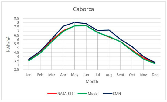
Figure 2.
Comparison between the SMN, NASA SSE, and the model for the station of Caborca.
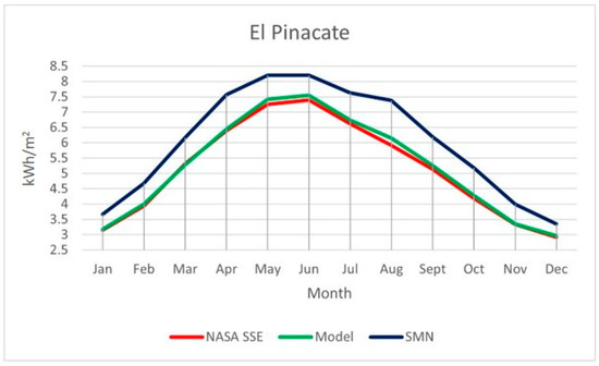
Figure 3.
Comparison between the SMN, NASA SSE, and the model for the station of El Pinacate.
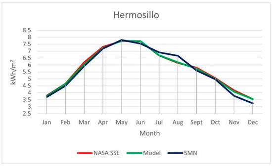
Figure 4.
Comparison between the SMN, NASA SSE, and the model for the station of Hermosillo.
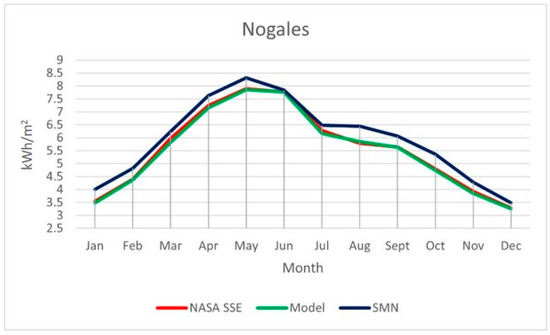
Figure 5.
Comparison between the SMN, NASA SSE, and the model for the station of Nogales.
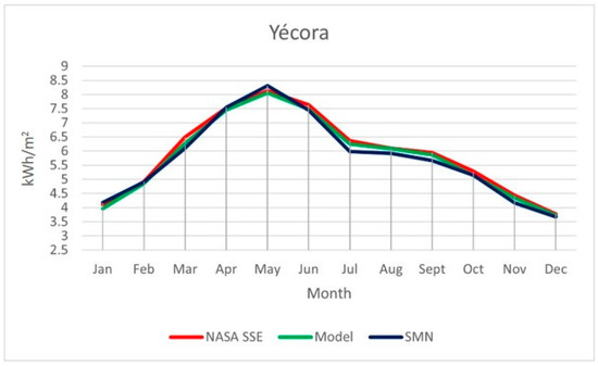
Figure 6.
Comparison between the SMN, NASA SSE, and the model for the station of Yécora.
In Figure 2, Figure 3, Figure 4, Figure 5 and Figure 6, the statement described by the statistical analysis was visually reinforced. A close trajectory for the values of NASA SSE (red) and the model (green) is visible in all the stations. However, the SMN (blue) maintains a close trajectory with small errors for the stations of Hermosillo and Yécora. These were the two stations with better performance in the model approximation for the other two references (NASA SSE and SMN). In the graphs, it can be seen in the case of Yécora that the model is closer to the SMN than NASA SEE. This explains why, in this case, the statistical metrics presented a better performance of the model with respect to the SMN compared to NASA SSE. The errors were wider in the case of Caborca and Nogales, with significant gaps between the red and green lines with respect to the blue line. The highest error was in El Pinacate with separate trajectories between the SMN and the other two sources of data. This means a significant standard deviation between NASA SSE and the model with respect to the SMN values in this station. Additionally, it merits noticing that the errors described by and in the statistical analysis described the direction of the error and magnitude for each month, where the SMN was taken as the reference for both. When the NASA SSE or the model values were smaller than the SMN, and were negatives, otherwise, they were positives. The magnitude of these parameters represents the gaps between the trajectories of the three data sources.
As a result of the obtained values in the comparative analysis, it can be stated that the model was quite accurate as an approximation of the values obtained from the NASA SSE database for latitudes of 32–26° N. The model had originally been tested at high latitudes in Russia at over 50° N. These results may imply that the model can be applied to any geographical point and obtain a close approximation of the total solar radiation available. However, more research in other world regions for latitudes further south is needed to ensure this statement.
4.4.2. Geographical Overview of Solar Resource and Opportunities of Solar Power in Sonora
A geographical information system (GIS) comparison analysis between solar total radiation calculated from the model and temperatures (maximum/minimum) for all municipalities in Sonora based on a series of heat maps is presented as a visualization tool of solar potential in Figure 7, Figure 8, Figure 9, Figure 10, Figure 11, Figure 12, Figure 13, Figure 14, Figure 15, Figure 16, Figure 17 and Figure 18. In these figures, the months of the year are represented in order from January to December, where Figure 7 represents January, Figure 8 represents February, and following this format until Figure 18 representing December. Further, each of the figures is separated into three GIS representations of the state of Sonora, where the first to the left is the average solar irradiance (kWh/m2), calculated by the model. The central heat map represents the average maximum temperatures (°C). Finally, the heat map on the right of each figure illustrates the average minimum temperatures (°C). A scale of colors was utilized to represent the values for each municipality in each GIS representation in Figure 7, Figure 8, Figure 9, Figure 10, Figure 11, Figure 12, Figure 13, Figure 14, Figure 15, Figure 16, Figure 17 and Figure 18. The coordinates together with the results of solar irradiance calculated by the model and from the NASA SSE database (for comparison), temperatures, surface albedo, and transparency index throughout the year for each municipality in the state can be found in Appendix A.
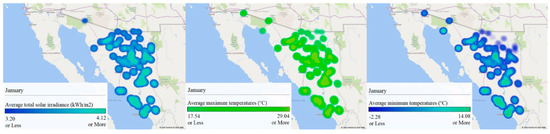
Figure 7.
GIS analysis of Sonora for January: (left) average total solar irradiance (kWh/m2), (center) maximum average temperatures (°C), and (right) minimum average temperatures (°C).
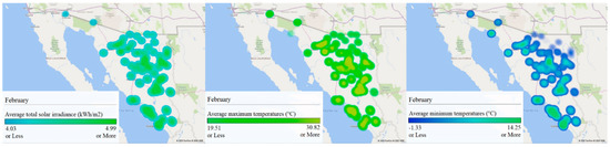
Figure 8.
GIS analysis of Sonora for February: (left) average solar total radiation (kWh/m2), (center) maximum average temperatures (°C), and (right) minimum average temperatures (°C).
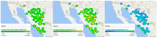
Figure 9.
GIS analysis of Sonora for March: (left) average total solar irradiance (kWh/m2), (center) maximum average temperatures (°C), and (right) minimum average temperatures (°C).
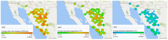
Figure 10.
GIS analysis of Sonora for April: (left) average total solar irradiance (kWh/m2), (center) maximum average temperatures (°C), and (right) minimum average temperatures (°C).
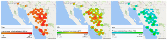
Figure 11.
GIS analysis of Sonora for May: (left) average total solar irradiance (kWh/m2), (center) maximum average temperatures (°C), and (right) minimum average temperatures (°C).
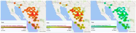
Figure 12.
GIS analysis of Sonora for June: (left) average total solar irradiance (kWh/m2), (center) maximum average temperatures (°C), and (right) minimum average temperatures (°C).
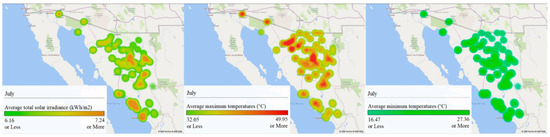
Figure 13.
GIS analysis of Sonora for July: (left) average total solar irradiance (kWh/m2), (center) maximum average temperatures (°C), and (right) minimum average temperatures (°C).
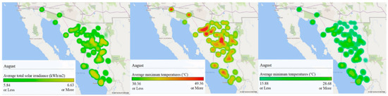
Figure 14.
GIS analysis of Sonora for August: (left) average total solar irradiance (kWh/m2), (center) maximum average temperatures (°C), and (right) minimum average temperatures (°C).
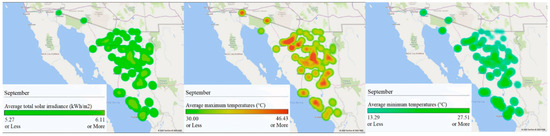
Figure 15.
GIS analysis of Sonora for September: (left) average total solar irradiance (kWh/m2), (center) maximum average temperatures (°C), and (right) minimum average temperatures (°C).
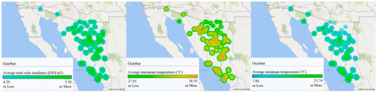
Figure 16.
GIS analysis of Sonora for October: (left) average total solar irradiance (kWh/m2), (center) maximum average temperatures (°C), and (right) minimum average temperatures (°C).
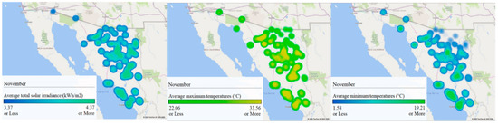
Figure 17.
GIS analysis of Sonora for November: (left) average total solar irradiance (kWh/m2), (center) maximum average temperatures (°C), and (right) minimum average temperatures (°C).
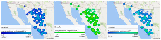
Figure 18.
GIS analysis of Sonora for December: (left) average total solar irradiance (kWh/m2), (center) maximum average temperatures (°C), and (right) minimum average temperatures (°C).
The geographical analysis showed high solar irradiance in Sonora throughout the year, with values over 2.99 kWh/m2 on average. The regions with constant higher values were the north-central, central, east, and southern regions of the state. However, some of these areas were also the hottest with average maximum temperatures over 40 °C during April–September, which may mean a significant economic cost due to the need for more modules or cooling systems to compensate for the loss of efficiency due to high temperatures. On the other hand, average minimum temperatures under 0 °C were presented in the northeast and eastern regions during December–February. This represents a good potential for solar development in the eastern region of the state because of less severe maximum temperatures and good solar irradiance on average. However, extreme average minimum temperatures must be considered during the design and sizing of solar photovoltaic projects. The main problem in the eastern region is the mountainous terrain, where any solar project must be carefully analyzed due to the space required. Finally, the western and northwest regions of the state were also worth consideration because, even though there are fewer solar resources compared to the central region, the solar irradiance in these regions is still high on average and the terrain is flatter than in other regions of the state, which facilitates the planning and installation of large-scale solar harvesting projects. Temperatures are also not so extreme, so better efficiency values in photovoltaic energy production are expected.
The results obtained in this GIS analysis provide a view and perspective of a great zone of opportunity in the northwest territory of Mexico for energy production based on the abundant solar resource available. This may represent a tremendous potential of local development of municipalities in the region and their decarbonization for electricity and heating production, which may mean a big reduction in its carbon footprint. This would imply a great economic development and possible energy exportation out of the region either to the United States or other regions of Mexico.
5. Conclusions
The accuracy of the model for the latitudes of the state of Sonora was proved and analyzed under several statistical metrics comparing it against real-time measurements from the stations of the Mexican meteorological network (SMN) and the satellite solar irradiance records from the NASA SSE database. The SMN meteorological stations available for a comparative analysis in the state were only 33.3% of the total. The rest of the stations presented important data gaps for the period 2015–2019 which discarded them as reliable reference sources. The performance obtained in the statistical analysis demonstrated satisfactory accuracy of the model for latitudes of 32–26° N. However, some differences were observed between NASA SSE and the model compared to real-time data from the SMN for certain meteorological stations. This may imply measurement errors or a need for calibration, but more research of equipment in the SMN stations must be conducted to ensure this statement.
A series of heat maps was utilized for comparing solar radiation against maximum and minimum temperatures in the municipalities in Sonora state. This geographical analysis highlighted that Sonora is a region with high radiation values in a range from 2.99 kWh/m2 to 8.07 kW/m2 during the year for all the municipalities calculated. The advantages and disadvantages were discussed and identified based on the range of annual temperatures for each region in the state. This analysis revealed regions of opportunities for decision-makers and stakeholders in different organizations, both public and private, interested in reducing the carbon footprint, providing an acceptable and wide vision for planning photovoltaic power projects in the region.
The extensive set of tests and results remark the non-complexity nature and accuracy of the applied mathematical model. It requires three inputs (surface albedo, clearness index, and geographical coordinates) for the calculation of solar radiation in a convenient and economically viable way. This research work concludes that the applied model could be used as a support or reference for the calculation of solar resources in a county, a state, or large areas of countries for decision making related to sustainable development policies aimed at solar energy harvesting systems and carbon footprint reduction.
Finally, as future work, it is proposed to continue calculating the amount of solar radiation, but in other latitudes of the planet to validate the model and the herein results. The outcomes of this work reinforce the potential of this approach as a tool to be applied during solar energy planning by local governments.
Author Contributions
Conceptualization, E.A.E.-V. and V.H.B.; data curation, E.A.E.-V.; formal analysis, E.A.E.-V.; funding acquisition, V.H.B., L.C.F.-H. and J.d.-J.L.-S.; investigation, E.A.E.-V. and V.H.B.; methodology, E.A.E.-V. and V.H.B.; project administration, E.A.E.-V. and V.H.B.; resources, E.A.E.-V. and V.H.B.; software, E.A.E.-V. and S.G.O.; supervision, V.H.B., L.C.F.-H. and J.d.-J.L.-S.; validation, E.A.E.-V., V.H.B. and S.G.O.; visualization, E.A.E.-V., V.H.B. and S.G.O.; writing—original draft, E.A.E.-V.; writing—review and editing, E.A.E.-V., V.H.B., S.G.O., L.C.F.-H. and J.d.-J.L.-S. All authors have read and agreed to the published version of the manuscript.
Funding
The APC was funded by CampusCity Initiative from the School of Engineering and Sciences at the Tecnologico de Monterrey.
Acknowledgments
A sincere thanks goes to the SMN for facilitating the data measured at its meteorological stations to carry out the statistical analysis presented in this research paper.
Conflicts of Interest
The authors declare no conflict of interest. The funders had no role in the design of the study; in the collection, analyses, or interpretation of data; in the writing of the manuscript, or in the decision to publish the results.
Nomenclature
| Symbols | |
| a | Hourly transparency coefficient first variable (dimensionless) |
| Ai | Anisotropic index (dimensionless) |
| Az | Solar azimuth (angle) |
| B | Equation of time coefficient (dimensionless) |
| b | Hourly transparency coefficient second variable (dimensionless) |
| df | T-Student degrees of freedom (dimensionless) |
| Dif GMT | Time zone hour difference with respect to Greenwich meridian (hours) |
| EoT | Equation of time (hours) |
| G | Total radiation arriving at an inclined surface (W/m2) |
| G0 | Hourly extra-atmospheric radiation arriving at a horizontal surface (W/m2) |
| GD | Hourly direct radiation arriving at a horizontal surface (W/m2) |
| GDH | Hourly diffuse radiation arriving at a horizontal surface (W/m2) |
| GH | Hourly total radiation arriving at a horizontal surface (W/m2) |
| Gm | Total solar irradiance measured on-site (W/m2) |
| GSC | Solar constant = 1367 W/m2 |
| h | Solar altitude angle |
| H | Average daily radiation arriving at a horizontal surface (Wh/m2) |
| H0 | Average daily extra-atmospheric insolation arriving at a horizontal surface (Wh/m2) |
| HD | Average daily diffuse radiation arriving at a horizontal surface (Wh/m2) |
| i | Number of the analyzed month |
| KD | Diffusion index (dimensionless) |
| KT | Clearness index (dimensionless) |
| Max. T | Maximum average temperature (°C) |
| Mean T | Mean average temperature (°C) |
| Min. T | Minimum average temperature (°C) |
| n | Number of months in the year |
| N | Day number |
| r | Correlation coefficient (dimensionless) |
| R2 | Coefficient of determination (dimensionless) |
| rd | Hourly diffuse coefficient (dimensionless) |
| rt | Hourly transparency coefficient (dimensionless) |
| t | T-Student distribution test (dimensionless) |
| Time hr | Time of the day in hours |
| VDC max inverter | Maximum DC voltage input of an inverter (Volts) |
| VDC string | DC voltage per string connected to an inverter (Volts) |
| Xi | Reference value for statistical analysis |
| Yi | Calculated value for statistical analysis |
| Greek letters | |
| Sunset hour angle | |
| Solar zenith angle | |
| δ | Declination angle |
| Ψ | Longitude |
| ω | Solar hour angle |
| Slope angle of the receiving surface with respect to the horizontal | |
| Surface azimuth angle | |
| Incidence angle | |
| Surface albedo (dimensionless) | |
| Latitude | |
| Abbreviations | |
| AC | Alternating current |
| CCS | Center for Climate Strategies |
| CEDES | Commission of Ecology and Sustainable Development of the State of Sonora |
| CEMIE-SOL | Mexican Centre of Innovation in Solar Energy |
| CONACYT | National Council for Science and Technology |
| CONAGUA | Mexican National Water Commission |
| DC | Direct current |
| EMAs | Automatic meteorological stations |
| ESIMEs | Synoptic meteorological stations |
| GHGs | Greenhouse gas emissions |
| GIS | Geographical information system |
| MAE | Mean absolute error (dimensionless) |
| MBE | Mean bias error (dimensionless) |
| MPE | Mean percentage error (%) |
| NASA | National Aeronautics and Space Administration |
| NASA SSE | NASA Surface Meteorology and Solar Energy |
| PV | Photovoltaic |
| RMSE | Root mean square error (dimensionless) |
| RPE | Relative percentage error (%) |
| SAM | Solar Advisor Model |
| SENER | Secretary of Energy |
| SMN | Mexican National Weather Service |
| SOLARGIS | Global Solar Atlas |
| UNAM | National Autonomous University of Mexico |
| UTC | Coordinated Universal Time |
| WMO | World Meteorological Organization |
Appendix A. Calculations of Solar Irradiance Parameters for All Municipalities in Sonora
Table A1 presents the solar irradiance in kWh/m2 calculated using the proposed model and from the satellite NASA SSE database for all the 72 municipalities in the state of Sonora. Further, surface albedo () and transparency index (Kt) are shown. These two parameters are dimensionless. Other important parameters illustrated are monthly maximum, mean, and minimum average temperatures in °C for each municipality.
Table A1.
Solar irradiance in kW/m2 from the model, the NASA SSE database, temperatures, surface albedo, and transparency index for each municipality in Sonora.
Table A1.
Solar irradiance in kW/m2 from the model, the NASA SSE database, temperatures, surface albedo, and transparency index for each municipality in Sonora.
| Municipality | Latitude | Longitude | Parameter | Month | Annual Average | |||||||||||
|---|---|---|---|---|---|---|---|---|---|---|---|---|---|---|---|---|
| Jan | Feb | Mar | Apr | May | Jun | Jul | Aug | Sept | Oct | Nov | Dec | |||||
| Aconchi | 29.82° N | 110.26° W | S. Albedo | 0.17 | 0.17 | 0.17 | 0.17 | 0.18 | 0.19 | 0.18 | 0.17 | 0.17 | 0.16 | 0.16 | 0.16 | |
| T. index (KT) | 0.63 | 0.64 | 0.69 | 0.71 | 0.7 | 0.68 | 0.6 | 0.59 | 0.62 | 0.65 | 0.65 | 0.63 | ||||
| NASA SSE | 3.8 | 4.66 | 6.19 | 7.31 | 7.72 | 7.71 | 6.69 | 6.14 | 5.81 | 5.06 | 4.17 | 3.54 | 5.73 | |||
| Model | 3.7 | 4.58 | 6.01 | 7.21 | 7.74 | 7.74 | 6.72 | 6.18 | 5.71 | 4.94 | 4.01 | 3.46 | 5.67 | |||
| Max. T (°C) | 25.05 | 27.12 | 32.28 | 37.57 | 42.47 | 46.55 | 40.64 | 37.85 | 38.38 | 35.77 | 29.78 | 24.57 | ||||
| Mean T (°C) | 11.6 | 13.24 | 17.01 | 21.65 | 26.57 | 31.39 | 29.75 | 28.09 | 26.71 | 22.1 | 16.07 | 11.44 | ||||
| Min. T (°C) | 3.44 | 4.06 | 5.99 | 9.05 | 13.27 | 18.65 | 21.51 | 20.85 | 18.48 | 13.01 | 7.58 | 3.69 | ||||
| Agua Prieta | 31.31° N | 109.66° W | S. Albedo | 0.15 | 0.16 | 0.16 | 0.16 | 0.17 | 0.18 | 0.17 | 0.16 | 0.16 | 0.15 | 0.15 | 0.14 | |
| T. index (KT) | 0.62 | 0.63 | 0.68 | 0.71 | 0.7 | 0.67 | 0.55 | 0.56 | 0.62 | 0.65 | 0.65 | 0.62 | ||||
| NASA SSE | 3.53 | 4.36 | 5.92 | 7.2 | 7.73 | 7.58 | 6.18 | 5.77 | 5.61 | 4.82 | 3.89 | 3.27 | 5.49 | |||
| Model | 3.49 | 4.38 | 5.81 | 7.16 | 7.75 | 7.66 | 6.17 | 5.85 | 5.63 | 4.81 | 3.85 | 3.25 | 5.48 | |||
| Max. T (°C) | 18.45 | 21.31 | 26.41 | 31.92 | 37.89 | 43.66 | 39.98 | 37.65 | 36.16 | 30.66 | 23.4 | 18.01 | ||||
| Mean T (°C) | 5.67 | 7.86 | 11.74 | 16.62 | 22.46 | 28.26 | 27.8 | 26.09 | 23.42 | 17.11 | 10.15 | 5.5 | ||||
| Min. T (°C) | −2.28 | −1.33 | 0.8 | 4.15 | 9.3 | 15.05 | 18.48 | 17.57 | 14.2 | 7.81 | 1.58 | −2.11 | ||||
| Álamos | 27.03° N | 109.03° W | S. Albedo | 0.12 | 0.12 | 0.12 | 0.12 | 0.13 | 0.13 | 0.14 | 0.13 | 0.13 | 0.11 | 0.11 | 0.12 | |
| T. index (KT) | 0.64 | 0.65 | 0.7 | 0.7 | 0.7 | 0.67 | 0.59 | 0.58 | 0.62 | 0.64 | 0.66 | 0.63 | ||||
| NASA SSE | 4.07 | 4.94 | 6.39 | 7.26 | 7.8 | 7.56 | 6.59 | 6.09 | 5.88 | 5.18 | 4.38 | 3.77 | 5.83 | |||
| Model | 4.04 | 4.9 | 6.28 | 7.19 | 7.72 | 7.55 | 6.56 | 6.1 | 5.84 | 5.08 | 4.35 | 3.75 | 5.78 | |||
| Max. T (°C) | 28.81 | 30.71 | 34.99 | 39.36 | 43.23 | 45.18 | 38.62 | 36.24 | 36.61 | 36.76 | 32.82 | 28.6 | ||||
| Mean T (°C) | 16.26 | 17.67 | 20.68 | 24.58 | 28.57 | 32.22 | 30.08 | 28.9 | 28.06 | 25.27 | 20.46 | 16.5 | ||||
| Min. T (°C) | 8.35 | 8.94 | 10.45 | 13.23 | 16.86 | 21.94 | 23.88 | 23.46 | 21.96 | 17.62 | 12.64 | 9.01 | ||||
| Altar | 30.74° N | 111.85° W | S. Albedo | 0.17 | 0.18 | 0.17 | 0.18 | 0.19 | 0.2 | 0.19 | 0.18 | 0.18 | 0.17 | 0.17 | 0.17 | |
| T. index (KT) | 0.63 | 0.64 | 0.68 | 0.7 | 0.69 | 0.66 | 0.58 | 0.58 | 0.62 | 0.64 | 0.64 | 0.63 | ||||
| NASA SSE | 3.65 | 4.54 | 6.01 | 7.2 | 7.55 | 7.48 | 6.49 | 5.93 | 5.66 | 4.88 | 3.99 | 3.4 | 5.57 | |||
| Model | 3.6 | 4.5 | 5.85 | 7.08 | 7.63 | 7.53 | 6.5 | 6.06 | 5.66 | 4.78 | 3.85 | 3.37 | 5.53 | |||
| Max. T (°C) | 24.94 | 27.01 | 31.97 | 36.97 | 42.64 | 47.49 | 44.43 | 42.45 | 41.55 | 36.55 | 29.85 | 24.4 | ||||
| Mean T (°C) | 11.82 | 13.41 | 17.07 | 21.36 | 26.65 | 31.7 | 31.92 | 30.72 | 28.53 | 22.63 | 16.34 | 11.55 | ||||
| Min. T (°C) | 3.98 | 4.58 | 6.58 | 9.41 | 13.76 | 18.73 | 22.7 | 22.39 | 19.6 | 13.55 | 8.17 | 4.04 | ||||
| Arivechi | 29° N | 109.47° W | S. Albedo | 0.14 | 0.14 | 0.14 | 0.15 | 0.15 | 0.16 | 0.15 | 0.14 | 0.14 | 0.14 | 0.13 | 0.13 | |
| T. index (KT) | 0.64 | 0.65 | 0.7 | 0.72 | 0.73 | 0.69 | 0.6 | 0.61 | 0.64 | 0.66 | 0.66 | 0.64 | ||||
| NASA SSE | 3.88 | 4.72 | 6.32 | 7.52 | 8.12 | 7.96 | 6.78 | 6.36 | 5.96 | 5.15 | 4.24 | 3.6 | 5.88 | |||
| Model | 3.84 | 4.73 | 6.15 | 7.34 | 8.07 | 7.83 | 6.7 | 6.4 | 5.93 | 5.08 | 4.15 | 3.6 | 5.82 | |||
| Max. T (°C) | 24.52 | 26.36 | 31.36 | 36.47 | 41.32 | 44.71 | 37.98 | 35.25 | 36.16 | 34.44 | 29.2 | 24.2 | ||||
| Mean T (°C) | 11.35 | 12.98 | 16.62 | 21.19 | 26.08 | 30.59 | 28.25 | 26.62 | 25.65 | 21.59 | 15.89 | 11.39 | ||||
| Min. T (°C) | 3.03 | 3.81 | 5.64 | 8.75 | 13.13 | 18.48 | 20.76 | 19.95 | 17.95 | 12.84 | 7.39 | 3.49 | ||||
| Arizpe | 30.35° N | 110.2° W | S. Albedo | 0.16 | 0.16 | 0.16 | 0.16 | 0.17 | 0.18 | 0.17 | 0.16 | 0.16 | 0.15 | 0.15 | 0.15 | |
| T. index (KT) | 0.63 | 0.64 | 0.69 | 0.72 | 0.72 | 0.68 | 0.58 | 0.58 | 0.63 | 0.65 | 0.66 | 0.63 | ||||
| NASA SSE | 3.71 | 4.58 | 6.15 | 7.39 | 7.97 | 7.85 | 6.54 | 6.06 | 5.8 | 4.99 | 4.09 | 3.46 | 5.72 | |||
| Model | 3.64 | 4.53 | 5.97 | 7.29 | 7.96 | 7.75 | 6.5 | 6.07 | 5.77 | 4.89 | 4.01 | 3.41 | 5.65 | |||
| Max. T (°C) | 22.72 | 24.97 | 30.01 | 35.37 | 40.59 | 45.29 | 40.25 | 37.71 | 37.55 | 33.77 | 27.45 | 22.28 | ||||
| Mean T (°C) | 9.48 | 11.21 | 14.94 | 19.62 | 24.86 | 30.03 | 28.82 | 27.22 | 25.43 | 20.13 | 13.88 | 9.32 | ||||
| Min. T (°C) | 1.35 | 2 | 3.94 | 7.06 | 11.56 | 17.07 | 20.19 | 19.51 | 16.81 | 10.97 | 5.36 | 1.58 | ||||
| Átil | 30.84° N | 111.6° W | S. Albedo | 0.17 | 0.18 | 0.17 | 0.18 | 0.19 | 0.2 | 0.19 | 0.18 | 0.18 | 0.17 | 0.17 | 0.17 | |
| T. index (KT) | 0.63 | 0.64 | 0.68 | 0.7 | 0.69 | 0.66 | 0.58 | 0.58 | 0.62 | 0.64 | 0.64 | 0.63 | ||||
| NASA SSE | 3.65 | 4.54 | 6.01 | 7.2 | 7.55 | 7.48 | 6.49 | 5.93 | 5.66 | 4.88 | 3.99 | 3.4 | 5.57 | |||
| Model | 3.59 | 4.49 | 5.85 | 7.08 | 7.63 | 7.53 | 6.5 | 6.06 | 5.66 | 4.78 | 3.84 | 3.36 | 5.53 | |||
| Max. T (°C) | 24.94 | 27.01 | 31.97 | 36.97 | 42.64 | 47.49 | 44.43 | 42.45 | 41.55 | 36.55 | 29.85 | 24.4 | ||||
| Mean T (°C) | 11.82 | 13.41 | 17.07 | 21.36 | 26.65 | 31.7 | 31.92 | 30.72 | 28.53 | 22.63 | 16.34 | 11.55 | ||||
| Min. T (°C) | 3.98 | 4.58 | 6.58 | 9.41 | 13.76 | 18.73 | 22.7 | 22.39 | 19.6 | 13.55 | 8.17 | 4.04 | ||||
| Bacadéhuachi | 29.8° N | 109.16° W | S. Albedo | 0.14 | 0.14 | 0.14 | 0.15 | 0.15 | 0.16 | 0.15 | 0.14 | 0.14 | 0.14 | 0.13 | 0.13 | |
| T. index (KT) | 0.64 | 0.65 | 0.7 | 0.72 | 0.73 | 0.69 | 0.6 | 0.61 | 0.64 | 0.66 | 0.66 | 0.64 | ||||
| NASA SSE | 3.88 | 4.72 | 6.32 | 7.52 | 8.12 | 7.96 | 6.78 | 6.36 | 5.96 | 5.15 | 4.24 | 3.6 | 5.88 | |||
| Model | 3.76 | 4.66 | 6.09 | 7.31 | 8.07 | 7.85 | 6.72 | 6.39 | 5.89 | 5.01 | 4.07 | 3.52 | 5.78 | |||
| Max. T (°C) | 23 | 24.89 | 29.82 | 34.96 | 40.07 | 44.07 | 38.36 | 35.9 | 36.15 | 33.3 | 27.66 | 22.6 | ||||
| Mean T (°C) | 10.01 | 11.67 | 15.29 | 19.91 | 25 | 29.78 | 27.97 | 26.4 | 25.04 | 20.41 | 14.5 | 9.98 | ||||
| Min. T (°C) | 1.73 | 2.54 | 4.36 | 7.52 | 12.04 | 17.43 | 19.99 | 19.21 | 16.92 | 11.54 | 5.97 | 2.13 | ||||
| Bacanora | 28.98° N | 109.42° W | S. Albedo | 0.14 | 0.14 | 0.14 | 0.15 | 0.15 | 0.16 | 0.16 | 0.15 | 0.14 | 0.13 | 0.13 | 0.13 | |
| T. index (KT) | 0.64 | 0.65 | 0.7 | 0.72 | 0.72 | 0.68 | 0.59 | 0.59 | 0.62 | 0.65 | 0.66 | 0.63 | ||||
| NASA SSE | 4 | 4.83 | 6.38 | 7.45 | 8.01 | 7.73 | 6.65 | 6.2 | 5.9 | 5.18 | 4.32 | 3.7 | 5.86 | |||
| Model | 3.84 | 4.73 | 6.15 | 7.34 | 7.96 | 7.72 | 6.59 | 6.19 | 5.75 | 5.01 | 4.15 | 3.55 | 5.75 | |||
| Max. T (°C) | 24.57 | 26.32 | 31.02 | 35.89 | 40.39 | 43.41 | 36.59 | 33.85 | 34.69 | 33.69 | 29.02 | 24.34 | ||||
| Mean T (°C) | 11.8 | 13.32 | 16.71 | 21.06 | 25.66 | 29.96 | 27.52 | 25.93 | 25.05 | 21.48 | 16.17 | 11.92 | ||||
| Min. T (°C) | 3.77 | 4.44 | 6.07 | 9.07 | 13.18 | 18.46 | 20.55 | 19.78 | 17.95 | 13.18 | 8.01 | 4.28 | ||||
| Bacerac | 30.35° N | 108.94° W | S. Albedo | 0.14 | 0.14 | 0.14 | 0.14 | 0.15 | 0.16 | 0.15 | 0.14 | 0.14 | 0.14 | 0.13 | 0.14 | |
| T. index (KT) | 0.63 | 0.64 | 0.69 | 0.71 | 0.7 | 0.66 | 0.55 | 0.56 | 0.62 | 0.65 | 0.66 | 0.63 | ||||
| NASA SSE | 3.7 | 4.51 | 6.12 | 7.3 | 7.82 | 7.52 | 6.21 | 5.83 | 5.7 | 4.95 | 4.07 | 3.42 | 5.6 | |||
| Model | 3.64 | 4.54 | 5.97 | 7.19 | 7.74 | 7.52 | 6.16 | 5.86 | 5.68 | 4.89 | 4.01 | 3.41 | 5.55 | |||
| Max. T (°C) | 17.54 | 19.51 | 23.73 | 28.32 | 33.41 | 38.07 | 34.66 | 33.2 | 32.11 | 27.95 | 22.06 | 17.3 | ||||
| Mean T (°C) | 6.06 | 7.72 | 10.93 | 15.22 | 20.22 | 25.21 | 24.52 | 23.36 | 21.33 | 16.21 | 10.31 | 6.08 | ||||
| Min. T (°C) | −1.42 | −0.65 | 0.86 | 3.93 | 8.42 | 13.64 | 16.47 | 15.88 | 13.29 | 7.83 | 2.32 | −1.1 | ||||
| Bacoachi | 30.63° N | 109.98° W | S. Albedo | 0.15 | 0.15 | 0.15 | 0.15 | 0.16 | 0.16 | 0.15 | 0.15 | 0.14 | 0.14 | 0.14 | 0.14 | |
| T. index (KT) | 0.64 | 0.64 | 0.7 | 0.72 | 0.72 | 0.68 | 0.57 | 0.58 | 0.62 | 0.65 | 0.66 | 0.63 | ||||
| NASA SSE | 3.74 | 4.55 | 6.17 | 7.44 | 8.01 | 7.81 | 6.45 | 6.05 | 5.78 | 5 | 4.12 | 3.45 | 5.71 | |||
| Model | 3.67 | 4.51 | 6.03 | 7.29 | 7.97 | 7.76 | 6.39 | 6.06 | 5.67 | 4.87 | 3.98 | 3.38 | 5.63 | |||
| Max. T (°C) | 20.03 | 22.66 | 27.68 | 33.16 | 38.86 | 44.3 | 40.07 | 37.77 | 36.67 | 31.72 | 24.87 | 19.63 | ||||
| Mean T (°C) | 6.99 | 9.01 | 12.8 | 17.64 | 23.29 | 28.86 | 28.03 | 26.39 | 24.04 | 18.1 | 11.44 | 6.86 | ||||
| Min. T (°C) | −1.19 | −0.32 | 1.69 | 5 | 9.97 | 15.68 | 18.93 | 18.1 | 14.98 | 8.78 | 2.77 | −0.95 | ||||
| Bácum | 27.54° N | 110.12° W | S. Albedo | 0.07 | 0.07 | 0.07 | 0.08 | 0.09 | 0.09 | 0.09 | 0.08 | 0.08 | 0.07 | 0.07 | 0.07 | |
| T. index (KT) | 0.65 | 0.66 | 0.71 | 0.71 | 0.73 | 0.71 | 0.65 | 0.63 | 0.65 | 0.67 | 0.66 | 0.63 | ||||
| NASA SSE | 4.14 | 4.99 | 6.5 | 7.44 | 8.12 | 8.16 | 7.36 | 6.69 | 6.25 | 5.44 | 4.44 | 3.79 | 6.11 | |||
| Model | 4.05 | 4.93 | 6.34 | 7.28 | 8.05 | 8.02 | 7.24 | 6.23 | 6.1 | 5.28 | 4.3 | 3.7 | 5.96 | |||
| Max. T (°C) | 29.04 | 30.82 | 35.08 | 39.2 | 42.95 | 46.01 | 41.07 | 38.9 | 39.54 | 38.59 | 33.56 | 28.88 | ||||
| Mean T (°C) | 17.34 | 18.66 | 21.63 | 25.28 | 29.19 | 33.23 | 32.23 | 31.16 | 30.45 | 27.24 | 21.92 | 17.65 | ||||
| Min. T (°C) | 10.17 | 10.76 | 12.39 | 15.02 | 18.58 | 23.49 | 26.05 | 25.86 | 24.49 | 19.99 | 14.74 | 10.88 | ||||
| Banámichi | 30.01° N | 110.24° W | S. Albedo | 0.16 | 0.16 | 0.16 | 0.16 | 0.17 | 0.18 | 0.17 | 0.16 | 0.16 | 0.15 | 0.15 | 0.15 | |
| T. index (KT) | 0.63 | 0.64 | 0.69 | 0.72 | 0.72 | 0.68 | 0.58 | 0.58 | 0.63 | 0.65 | 0.66 | 0.63 | ||||
| NASA SSE | 3.71 | 4.58 | 6.15 | 7.39 | 7.97 | 7.85 | 6.54 | 6.06 | 5.8 | 4.99 | 4.09 | 3.46 | 5.72 | |||
| Model | 3.68 | 4.57 | 5.99 | 7.31 | 7.96 | 7.74 | 6.49 | 6.07 | 5.79 | 4.92 | 4.05 | 3.44 | 5.67 | |||
| Max. T (°C) | 22.72 | 24.97 | 30.01 | 35.37 | 40.59 | 45.29 | 40.25 | 37.71 | 37.55 | 33.77 | 27.45 | 22.28 | ||||
| Mean T (°C) | 9.48 | 11.21 | 14.94 | 19.62 | 24.86 | 30.03 | 28.82 | 27.22 | 25.43 | 20.13 | 13.88 | 9.32 | ||||
| Min. T (°C) | 1.35 | 2 | 3.94 | 7.06 | 11.56 | 17.07 | 20.19 | 19.51 | 16.81 | 10.97 | 5.36 | 1.58 | ||||
| Baviácora | 29.7° N | 110.19° W | S. Albedo | 0.17 | 0.17 | 0.17 | 0.17 | 0.18 | 0.19 | 0.18 | 0.17 | 0.17 | 0.16 | 0.16 | 0.16 | |
| T. index (KT) | 0.63 | 0.64 | 0.69 | 0.71 | 0.7 | 0.68 | 0.6 | 0.59 | 0.62 | 0.65 | 0.65 | 0.63 | ||||
| NASA SSE | 3.8 | 4.66 | 6.19 | 7.31 | 7.72 | 7.71 | 6.69 | 6.14 | 5.81 | 5.06 | 4.17 | 3.54 | 5.73 | |||
| Model | 3.71 | 4.59 | 6.01 | 7.21 | 7.74 | 7.74 | 6.71 | 6.18 | 5.71 | 4.95 | 4.02 | 3.48 | 5.67 | |||
| Max. T (°C) | 25.05 | 27.12 | 32.28 | 37.57 | 42.47 | 46.55 | 40.64 | 37.85 | 38.38 | 35.77 | 29.78 | 24.57 | ||||
| Mean T (°C) | 11.6 | 13.24 | 17.01 | 21.65 | 26.57 | 31.39 | 29.75 | 28.09 | 26.71 | 22.1 | 16.07 | 11.44 | ||||
| Min. T (°C) | 3.44 | 4.06 | 5.99 | 9.05 | 13.27 | 18.65 | 21.51 | 20.85 | 18.48 | 13.01 | 7.58 | 3.69 | ||||
| Bavispe | 30.48° N | 108.92° W | S. Albedo | 0.14 | 0.14 | 0.14 | 0.14 | 0.15 | 0.16 | 0.15 | 0.14 | 0.14 | 0.14 | 0.13 | 0.14 | |
| T. index (KT) | 0.63 | 0.64 | 0.69 | 0.71 | 0.7 | 0.66 | 0.55 | 0.56 | 0.62 | 0.65 | 0.66 | 0.63 | ||||
| NASA SSE | 3.7 | 4.51 | 6.12 | 7.3 | 7.82 | 7.52 | 6.21 | 5.83 | 5.7 | 4.95 | 4.07 | 3.42 | 5.6 | |||
| Model | 3.63 | 4.52 | 5.96 | 7.19 | 7.74 | 7.53 | 6.16 | 5.86 | 5.67 | 4.88 | 4 | 3.39 | 5.54 | |||
| Max. T (°C) | 17.54 | 19.51 | 23.73 | 28.32 | 33.41 | 38.07 | 34.66 | 33.2 | 32.11 | 27.95 | 22.06 | 17.3 | ||||
| Mean T (°C) | 6.06 | 7.72 | 10.93 | 15.22 | 20.22 | 25.21 | 24.52 | 23.36 | 21.33 | 16.21 | 10.31 | 6.08 | ||||
| Min. T (°C) | −1.42 | −0.65 | 0.86 | 3.93 | 8.42 | 13.64 | 16.47 | 15.88 | 13.29 | 7.83 | 2.32 | −1.1 | ||||
| Benito Juárez | 27.28° N | 110.01° W | S. Albedo | 0.07 | 0.07 | 0.07 | 0.08 | 0.09 | 0.09 | 0.09 | 0.08 | 0.08 | 0.07 | 0.07 | 0.07 | |
| T. index (KT) | 0.65 | 0.66 | 0.71 | 0.71 | 0.73 | 0.71 | 0.65 | 0.63 | 0.65 | 0.67 | 0.66 | 0.63 | ||||
| NASA SSE | 4.14 | 4.99 | 6.5 | 7.44 | 8.12 | 8.16 | 7.36 | 6.69 | 6.25 | 5.44 | 4.44 | 3.79 | 6.11 | |||
| Model | 4.08 | 4.96 | 6.36 | 7.28 | 8.05 | 8.01 | 7.23 | 6.63 | 6.11 | 5.3 | 4.33 | 3.73 | 6.01 | |||
| Max. T (°C) | 25.85 | 26.93 | 29.98 | 33.22 | 36.64 | 39.56 | 37.22 | 36.25 | 36.54 | 35.47 | 30.84 | 26.46 | ||||
| Mean T (°C) | 18.15 | 18.87 | 21.02 | 23.99 | 27.54 | 31.09 | 31.29 | 31.05 | 30.56 | 27.99 | 23.18 | 19.12 | ||||
| Min. T (°C) | 13.48 | 13.74 | 15.04 | 17.41 | 20.74 | 24.87 | 27.31 | 27.66 | 26.79 | 23.35 | 18.51 | 14.72 | ||||
| Benjamín Hill | 29.88° N | 111.35° W | S. Albedo | 0.15 | 0.16 | 0.16 | 0.16 | 0.17 | 0.18 | 0.17 | 0.16 | 0.16 | 0.15 | 0.15 | 0.15 | |
| T. index (KT) | 0.62 | 0.64 | 0.68 | 0.69 | 0.69 | 0.66 | 0.59 | 0.59 | 0.62 | 0.64 | 0.64 | 0.62 | ||||
| NASA SSE | 3.72 | 4.6 | 6.09 | 7.09 | 7.54 | 7.47 | 6.6 | 6.04 | 5.78 | 4.94 | 4.07 | 3.47 | 5.62 | |||
| Model | 3.63 | 4.58 | 5.91 | 7.01 | 7.63 | 7.51 | 6.6 | 6.18 | 5.7 | 4.86 | 3.94 | 3.4 | 5.58 | |||
| Max. T (°C) | 26.42 | 28.52 | 33.43 | 38.42 | 43.34 | 47.68 | 42.84 | 40.44 | 40.31 | 36.76 | 30.77 | 25.83 | ||||
| Mean T (°C) | 13.13 | 14.68 | 18.28 | 22.58 | 27.34 | 32.17 | 31.12 | 29.68 | 28.06 | 23.08 | 17.28 | 12.87 | ||||
| Min. T (°C) | 5.3 | 5.81 | 7.7 | 10.48 | 14.39 | 19.5 | 22.58 | 22.13 | 19.79 | 14.22 | 9.18 | 5.42 | ||||
| Caborca | 30.34° N | 112.55° W | S. Albedo | 0.1 | 0.11 | 0.11 | 0.12 | 0.12 | 0.12 | 0.12 | 0.11 | 0.11 | 0.1 | 0.1 | 0.1 | |
| T. index (KT) | 0.62 | 0.63 | 0.67 | 0.69 | 0.69 | 0.67 | 0.61 | 0.61 | 0.63 | 0.63 | 0.62 | 0.6 | ||||
| NASA SSE | 3.59 | 4.47 | 5.93 | 7.08 | 7.61 | 7.68 | 6.88 | 6.31 | 5.78 | 4.79 | 3.87 | 3.29 | 5.61 | |||
| Model | 3.59 | 4.47 | 5.8 | 6.99 | 7.63 | 7.64 | 6.83 | 6.38 | 5.77 | 4.74 | 3.87 | 3.25 | 5.58 | |||
| Max. T (°C) | 22.78 | 23.9 | 27.19 | 30.6 | 34.52 | 38.41 | 39.09 | 38.88 | 38.3 | 34.18 | 28.29 | 23.23 | ||||
| Mean T (°C) | 14.84 | 15.71 | 18.2 | 21.31 | 25.13 | 29.07 | 31.48 | 31.67 | 30.3 | 25.64 | 20.15 | 15.59 | ||||
| Min. T (°C) | 10.07 | 10.39 | 11.98 | 14.35 | 17.69 | 21.53 | 25.9 | 26.63 | 25 | 20.19 | 15.19 | 11.04 | ||||
| Cajeme | 27.58° N | 110.38° W | S. Albedo | 0.07 | 0.07 | 0.07 | 0.08 | 0.09 | 0.09 | 0.09 | 0.08 | 0.08 | 0.07 | 0.07 | 0.07 | |
| T. index (KT) | 0.65 | 0.66 | 0.71 | 0.71 | 0.73 | 0.71 | 0.65 | 0.63 | 0.65 | 0.67 | 0.66 | 0.63 | ||||
| NASA SSE | 4.14 | 4.99 | 6.5 | 7.44 | 8.12 | 8.16 | 7.36 | 6.69 | 6.25 | 5.44 | 4.44 | 3.79 | 6.11 | |||
| Model | 4.05 | 4.93 | 6.34 | 7.28 | 8.05 | 8.02 | 7.24 | 6.62 | 6.09 | 5.28 | 4.3 | 3.7 | 5.99 | |||
| Max. T (°C) | 29.04 | 30.82 | 35.08 | 39.2 | 42.95 | 46.01 | 41.07 | 38.9 | 39.54 | 38.59 | 33.56 | 28.88 | ||||
| Mean T (°C) | 17.34 | 18.66 | 21.63 | 25.28 | 29.19 | 33.23 | 32.23 | 31.16 | 30.45 | 27.24 | 21.92 | 17.65 | ||||
| Min. T (°C) | 10.17 | 10.76 | 12.39 | 15.02 | 18.58 | 23.49 | 26.05 | 25.86 | 24.49 | 19.99 | 14.74 | 10.88 | ||||
| Cananea | 31° N | 110.35° W | S. Albedo | 0.16 | 0.16 | 0.16 | 0.17 | 0.18 | 0.18 | 0.17 | 0.16 | 0.16 | 0.15 | 0.16 | 0.15 | |
| T. index (KT) | 0.62 | 0.63 | 0.68 | 0.71 | 0.71 | 0.68 | 0.55 | 0.56 | 0.62 | 0.64 | 0.65 | 0.62 | ||||
| NASA SSE | 3.55 | 4.4 | 5.97 | 7.25 | 7.9 | 7.77 | 6.28 | 5.78 | 5.64 | 4.79 | 3.93 | 3.29 | 5.55 | |||
| Model | 3.52 | 4.41 | 5.84 | 7.17 | 7.86 | 7.77 | 6.17 | 5.85 | 5.65 | 4.76 | 3.89 | 3.29 | 5.52 | |||
| Max. T (°C) | 18.71 | 21.37 | 26.32 | 31.68 | 37.62 | 43.27 | 39.65 | 37.44 | 36.08 | 30.64 | 23.57 | 18.26 | ||||
| Mean T (°C) | 5.93 | 7.92 | 11.66 | 16.38 | 22.14 | 27.88 | 27.53 | 25.92 | 23.33 | 17.05 | 10.29 | 5.73 | ||||
| Min. T (°C) | −1.94 | −1.17 | 0.83 | 4 | 9 | 14.67 | 18.3 | 17.49 | 14.15 | 7.8 | 1.82 | −1.81 | ||||
| Carbó | 29.68° N | 110.98° W | S. Albedo | 0.17 | 0.17 | 0.17 | 0.17 | 0.18 | 0.19 | 0.18 | 0.17 | 0.17 | 0.16 | 0.16 | 0.16 | |
| T. index (KT) | 0.63 | 0.64 | 0.69 | 0.71 | 0.7 | 0.68 | 0.6 | 0.59 | 0.62 | 0.65 | 0.65 | 0.63 | ||||
| NASA SSE | 3.8 | 4.66 | 6.19 | 7.31 | 7.72 | 7.71 | 6.69 | 6.14 | 5.81 | 5.06 | 4.17 | 3.54 | 5.73 | |||
| Model | 3.71 | 4.6 | 6.02 | 7.21 | 7.74 | 7.74 | 6.71 | 6.18 | 5.71 | 4.95 | 4.02 | 3.48 | 5.67 | |||
| Max. T (°C) | 25.93 | 28.02 | 33.03 | 38.08 | 42.8 | 46.96 | 41.81 | 39.41 | 39.59 | 36.53 | 30.54 | 25.43 | ||||
| Mean T (°C) | 12.65 | 14.23 | 17.91 | 22.34 | 27.06 | 31.88 | 30.63 | 29.17 | 27.67 | 22.93 | 17.01 | 12.46 | ||||
| Min. T (°C) | 4.76 | 5.29 | 7.19 | 10.07 | 14.03 | 19.28 | 22.27 | 21.75 | 19.43 | 14 | 8.8 | 4.97 | ||||
| Cucurpe | 30.33° N | 110.72° W | S. Albedo | 0.16 | 0.16 | 0.16 | 0.16 | 0.17 | 0.18 | 0.17 | 0.16 | 0.16 | 0.15 | 0.15 | 0.15 | |
| T. index (KT) | 0.63 | 0.64 | 0.69 | 0.72 | 0.72 | 0.68 | 0.58 | 0.58 | 0.63 | 0.65 | 0.66 | 0.63 | ||||
| NASA SSE | 3.71 | 4.58 | 6.15 | 7.39 | 7.97 | 7.85 | 6.54 | 6.06 | 5.8 | 4.99 | 4.09 | 3.46 | 5.72 | |||
| Model | 3.65 | 4.54 | 5.97 | 7.3 | 7.96 | 7.75 | 6.5 | 6.07 | 5.77 | 4.89 | 4.01 | 3.41 | 5.65 | |||
| Max. T (°C) | 23.67 | 25.83 | 30.82 | 36 | 41.07 | 45.66 | 40.94 | 38.66 | 38.47 | 34.63 | 28.36 | 23.22 | ||||
| Mean T (°C) | 10.53 | 12.15 | 15.84 | 20.34 | 25.43 | 30.49 | 29.46 | 28.02 | 26.26 | 21.01 | 14.88 | 10.35 | ||||
| Min. T (°C) | 2.61 | 3.15 | 5.08 | 8.04 | 12.34 | 17.66 | 20.83 | 20.31 | 17.71 | 11.97 | 6.61 | 2.8 | ||||
| Cumpas | 30.34° N | 110.5° W | S. Albedo | 0.16 | 0.16 | 0.16 | 0.16 | 0.17 | 0.18 | 0.17 | 0.16 | 0.16 | 0.15 | 0.15 | 0.15 | |
| T. index (KT) | 0.63 | 0.64 | 0.69 | 0.72 | 0.72 | 0.68 | 0.58 | 0.58 | 0.63 | 0.65 | 0.66 | 0.63 | ||||
| NASA SSE | 3.71 | 4.58 | 6.15 | 7.39 | 7.97 | 7.85 | 6.54 | 6.06 | 5.8 | 4.99 | 4.09 | 3.46 | 5.72 | |||
| Model | 3.65 | 4.54 | 5.97 | 7.29 | 7.96 | 7.75 | 6.5 | 6.07 | 5.77 | 4.89 | 4.01 | 3.41 | 5.65 | |||
| Max. T (°C) | 22.72 | 24.97 | 30.01 | 35.37 | 40.59 | 45.29 | 40.25 | 37.71 | 37.55 | 33.77 | 27.45 | 22.28 | ||||
| Mean T (°C) | 9.48 | 11.21 | 14.94 | 19.62 | 24.86 | 30.03 | 28.82 | 27.22 | 25.43 | 20.13 | 13.88 | 9.32 | ||||
| Min. T (°C) | 1.35 | 2 | 3.94 | 7.06 | 11.56 | 17.07 | 20.19 | 19.51 | 16.81 | 10.97 | 5.36 | 1.58 | ||||
| Divisaderos | 29.62° N | 109.48° W | S. Albedo | 0.14 | 0.14 | 0.14 | 0.15 | 0.15 | 0.16 | 0.15 | 0.14 | 0.14 | 0.14 | 0.13 | 0.13 | |
| T. index (KT) | 0.64 | 0.65 | 0.7 | 0.72 | 0.73 | 0.69 | 0.6 | 0.61 | 0.64 | 0.66 | 0.66 | 0.64 | ||||
| NASA SSE | 3.88 | 4.72 | 6.32 | 7.52 | 8.12 | 7.96 | 6.78 | 6.36 | 5.96 | 5.15 | 4.24 | 3.6 | 5.88 | |||
| Model | 3.78 | 4.67 | 6.11 | 7.32 | 8.07 | 7.85 | 6.71 | 6.39 | 5.9 | 5.03 | 4.09 | 3.54 | 5.79 | |||
| Max. T (°C) | 23 | 24.89 | 29.82 | 34.96 | 40.07 | 44.07 | 38.36 | 35.9 | 36.15 | 33.3 | 27.66 | 22.6 | ||||
| Mean T (°C) | 10.01 | 11.67 | 15.29 | 19.91 | 25 | 29.78 | 27.97 | 26.4 | 25.04 | 20.41 | 14.5 | 9.98 | ||||
| Min. T (°C) | 1.73 | 2.54 | 4.36 | 7.52 | 12.04 | 17.43 | 19.99 | 19.21 | 16.92 | 11.54 | 5.97 | 2.13 | ||||
| Empalme | 28° N | 110.85° W | S. Albedo | 0.16 | 0.16 | 0.16 | 0.16 | 0.17 | 0.18 | 0.17 | 0.17 | 0.17 | 0.16 | 0.15 | 0.15 | |
| T. index (KT) | 0.62 | 0.63 | 0.68 | 0.68 | 0.68 | 0.65 | 0.58 | 0.57 | 0.61 | 0.63 | 0.64 | 0.62 | ||||
| NASA SSE | 3.84 | 4.68 | 6.14 | 6.99 | 7.41 | 7.22 | 6.44 | 5.89 | 5.68 | 4.96 | 4.16 | 3.57 | 5.58 | |||
| Model | 3.82 | 4.67 | 6.04 | 6.96 | 7.51 | 7.35 | 6.47 | 5.99 | 5.7 | 4.93 | 4.12 | 3.59 | 5.60 | |||
| Max. T (°C) | 27.85 | 29.6 | 33.74 | 37.96 | 42.01 | 45.45 | 41.33 | 39.31 | 39.62 | 37.28 | 31.98 | 27.42 | ||||
| Mean T (°C) | 16.1 | 17.48 | 20.44 | 24.17 | 28.23 | 32.48 | 32.01 | 30.96 | 29.96 | 25.88 | 20.38 | 16.15 | ||||
| Min. T (°C) | 8.89 | 9.49 | 11.09 | 13.67 | 17.29 | 22.27 | 25.38 | 25.23 | 23.61 | 18.46 | 13.18 | 9.36 | ||||
| Etchojoa | 26.9° N | 109.72° W | S. Albedo | 0.07 | 0.07 | 0.07 | 0.08 | 0.09 | 0.09 | 0.1 | 0.09 | 0.08 | 0.07 | 0.07 | 0.07 | |
| T. index (KT) | 0.65 | 0.66 | 0.7 | 0.71 | 0.73 | 0.7 | 0.64 | 0.62 | 0.64 | 0.66 | 0.66 | 0.63 | ||||
| NASA SSE | 4.24 | 5.08 | 6.51 | 7.39 | 8.08 | 7.94 | 7.18 | 6.59 | 6.15 | 5.46 | 4.52 | 3.89 | 6.09 | |||
| Model | 4.12 | 4.99 | 6.29 | 7.29 | 8.05 | 7.89 | 7.11 | 6.53 | 6.03 | 5.25 | 4.36 | 3.77 | 5.97 | |||
| Max. T (°C) | 24.83 | 25.77 | 28.41 | 31.5 | 34.84 | 37.28 | 35.18 | 34.52 | 34.59 | 33.85 | 29.78 | 25.61 | ||||
| Mean T (°C) | 18.2 | 18.78 | 20.68 | 23.52 | 26.93 | 30.18 | 30.42 | 30.39 | 29.91 | 27.69 | 23.27 | 19.32 | ||||
| Min. T (°C) | 14.08 | 14.25 | 15.38 | 17.73 | 20.97 | 24.91 | 27.18 | 27.62 | 26.85 | 23.79 | 19.21 | 15.45 | ||||
| Fronteras | 30.91° N | 109.6° W | S. Albedo | 0.15 | 0.15 | 0.15 | 0.15 | 0.16 | 0.16 | 0.15 | 0.15 | 0.14 | 0.14 | 0.14 | 0.14 | |
| T. index (KT) | 0.64 | 0.64 | 0.7 | 0.72 | 0.72 | 0.68 | 0.57 | 0.58 | 0.62 | 0.65 | 0.66 | 0.63 | ||||
| NASA SSE | 3.74 | 4.55 | 6.17 | 7.44 | 8.01 | 7.81 | 6.45 | 6.05 | 5.78 | 5 | 4.12 | 3.45 | 5.71 | |||
| Model | 3.64 | 4.48 | 6.01 | 7.28 | 7.97 | 7.76 | 6.39 | 6.06 | 5.65 | 4.85 | 3.95 | 3.35 | 5.62 | |||
| Max. T (°C) | 20.03 | 22.66 | 27.68 | 33.16 | 38.86 | 44.3 | 40.07 | 37.77 | 36.67 | 31.72 | 24.87 | 19.63 | ||||
| Mean T (°C) | 6.99 | 9.01 | 12.8 | 17.64 | 23.29 | 28.86 | 28.03 | 26.39 | 24.04 | 18.1 | 11.44 | 6.86 | ||||
| Min. T (°C) | −1.19 | −0.32 | 1.69 | 5 | 9.97 | 15.68 | 18.93 | 18.1 | 14.98 | 8.78 | 2.77 | −0.95 | ||||
| General Plutarco Elías Calles | 32.01° N | 113.16° W | S. Albedo | 0.21 | 0.21 | 0.21 | 0.22 | 0.23 | 0.23 | 0.23 | 0.23 | 0.23 | 0.21 | 0.21 | 0.21 | |
| T. index (KT) | 0.6 | 0.61 | 0.64 | 0.66 | 0.68 | 0.68 | 0.62 | 0.6 | 0.6 | 0.61 | 0.62 | 0.6 | ||||
| NASA SSE | 3.29 | 4.12 | 5.41 | 6.59 | 7.53 | 7.73 | 6.97 | 6.16 | 5.33 | 4.41 | 3.59 | 3.03 | 5.35 | |||
| Model | 3.31 | 4.18 | 5.43 | 6.63 | 7.53 | 7.79 | 6.97 | 6.25 | 5.42 | 4.46 | 3.61 | 3.08 | 5.39 | |||
| Max. T (°C) | 23.83 | 26.47 | 31.78 | 36.9 | 43.01 | 48.25 | 48.61 | 47.3 | 45.28 | 38.23 | 29.62 | 23 | ||||
| Mean T (°C) | 11.36 | 13.42 | 17.44 | 21.98 | 27.61 | 32.68 | 35.16 | 34.35 | 31.22 | 23.98 | 16.37 | 10.83 | ||||
| Min. T (°C) | 3.92 | 4.86 | 7.27 | 10.39 | 15.03 | 19.78 | 24.85 | 24.92 | 21.54 | 14.65 | 8.33 | 3.67 | ||||
| Granados | 29.86° N | 109.33° W | S. Albedo | 0.14 | 0.14 | 0.14 | 0.15 | 0.15 | 0.16 | 0.15 | 0.14 | 0.14 | 0.14 | 0.13 | 0.13 | |
| T. index (KT) | 0.64 | 0.65 | 0.7 | 0.72 | 0.73 | 0.69 | 0.6 | 0.61 | 0.64 | 0.66 | 0.66 | 0.64 | ||||
| NASA SSE | 3.88 | 4.72 | 6.32 | 7.52 | 8.12 | 7.96 | 6.78 | 6.36 | 5.96 | 5.15 | 4.24 | 3.6 | 5.88 | |||
| Model | 3.75 | 4.65 | 6.09 | 7.31 | 8.07 | 7.85 | 6.72 | 6.39 | 5.89 | 5.01 | 4.06 | 3.51 | 5.78 | |||
| Max. T (°C) | 23 | 24.89 | 29.82 | 34.96 | 40.07 | 44.07 | 38.36 | 35.9 | 36.15 | 33.3 | 27.66 | 22.6 | ||||
| Mean T (°C) | 10.01 | 11.67 | 15.29 | 19.91 | 25 | 29.78 | 27.97 | 26.4 | 25.04 | 20.41 | 14.5 | 9.98 | ||||
| Min. T (°C) | 1.73 | 2.54 | 4.36 | 7.52 | 12.04 | 17.43 | 19.99 | 19.21 | 16.92 | 11.54 | 5.97 | 2.13 | ||||
| Guaymas | 28° N | 111.07° W | S. Albedo | 0.12 | 0.12 | 0.11 | 0.13 | 0.14 | 0.14 | 0.14 | 0.14 | 0.14 | 0.12 | 0.12 | 0.12 | |
| T. index (KT) | 0.64 | 0.65 | 0.69 | 0.71 | 0.71 | 0.69 | 0.63 | 0.61 | 0.64 | 0.65 | 0.65 | 0.63 | ||||
| NASA SSE | 3.91 | 4.79 | 6.28 | 7.33 | 7.88 | 7.88 | 6.99 | 6.37 | 6 | 5.12 | 4.22 | 3.63 | 5.87 | |||
| Model | 3.94 | 4.82 | 6.13 | 7.26 | 7.84 | 7.81 | 7.02 | 6.41 | 5.98 | 5.09 | 4.19 | 3.65 | 5.85 | |||
| Max. T (°C) | 24.49 | 25.7 | 28.77 | 32.1 | 36.09 | 40.14 | 38.64 | 37.41 | 37.39 | 34.6 | 29.17 | 24.67 | ||||
| Mean T (°C) | 16.25 | 17.24 | 19.49 | 22.58 | 26.5 | 30.74 | 31.61 | 31.18 | 30.29 | 26.39 | 20.96 | 16.79 | ||||
| Min. T (°C) | 11.05 | 11.51 | 12.87 | 15.24 | 18.8 | 23.34 | 26.69 | 26.99 | 25.68 | 21.03 | 15.77 | 11.89 | ||||
| Hermosillo | 29.17° N | 111.03° W | S. Albedo | 0.15 | 0.16 | 0.16 | 0.16 | 0.17 | 0.18 | 0.17 | 0.16 | 0.16 | 0.15 | 0.15 | 0.15 | |
| T. index (KT) | 0.62 | 0.64 | 0.68 | 0.69 | 0.69 | 0.66 | 0.59 | 0.59 | 0.62 | 0.64 | 0.64 | 0.62 | ||||
| NASA SSE | 3.72 | 4.6 | 6.09 | 7.09 | 7.54 | 7.47 | 6.6 | 6.04 | 5.78 | 4.94 | 4.07 | 3.47 | 5.62 | |||
| Model | 3.71 | 4.64 | 5.96 | 7.03 | 7.63 | 7.5 | 6.59 | 6.19 | 5.74 | 4.91 | 4.01 | 3.48 | 5.62 | |||
| Max. T (°C) | 28.04 | 30.11 | 34.84 | 39.55 | 44.18 | 48.48 | 43.93 | 41.44 | 41.49 | 38.14 | 32.23 | 27.38 | ||||
| Mean T (°C) | 14.85 | 16.43 | 19.9 | 24.03 | 28.52 | 33.31 | 32.61 | 31.19 | 29.74 | 24.84 | 18.98 | 14.61 | ||||
| Min. T (°C) | 7.04 | 7.62 | 9.45 | 12.13 | 15.85 | 21.01 | 24.39 | 24 | 21.84 | 16.21 | 11 | 7.23 | ||||
| Huachinera | 30.21° N | 108.97° W | S. Albedo | 0.14 | 0.14 | 0.14 | 0.14 | 0.15 | 0.16 | 0.15 | 0.14 | 0.14 | 0.14 | 0.13 | 0.14 | |
| T. index (KT) | 0.63 | 0.64 | 0.69 | 0.71 | 0.7 | 0.66 | 0.55 | 0.56 | 0.62 | 0.65 | 0.66 | 0.63 | ||||
| NASA SSE | 3.7 | 4.51 | 6.12 | 7.3 | 7.82 | 7.52 | 6.21 | 5.83 | 5.7 | 4.95 | 4.07 | 3.42 | 5.6 | |||
| Model | 3.66 | 4.55 | 5.98 | 7.2 | 7.74 | 7.52 | 6.16 | 5.86 | 5.69 | 4.9 | 4.03 | 3.42 | 5.56 | |||
| Max. T (°C) | 17.54 | 19.51 | 23.73 | 28.32 | 33.41 | 38.07 | 34.66 | 33.2 | 32.11 | 27.95 | 22.06 | 17.3 | ||||
| Mean T (°C) | 6.06 | 7.72 | 10.93 | 15.22 | 20.22 | 25.21 | 24.52 | 23.36 | 21.33 | 16.21 | 10.31 | 6.08 | ||||
| Min. T (°C) | −1.42 | −0.65 | 0.86 | 3.93 | 8.42 | 13.64 | 16.47 | 15.88 | 13.29 | 7.83 | 2.32 | −1.1 | ||||
| Huásabas | 29.91° N | 109.32° W | S. Albedo | 0.14 | 0.14 | 0.14 | 0.15 | 0.15 | 0.16 | 0.15 | 0.14 | 0.14 | 0.14 | 0.13 | 0.13 | |
| T. index (KT) | 0.64 | 0.65 | 0.7 | 0.72 | 0.73 | 0.69 | 0.6 | 0.61 | 0.64 | 0.66 | 0.66 | 0.64 | ||||
| NASA SSE | 3.88 | 4.72 | 6.32 | 7.52 | 8.12 | 7.96 | 6.78 | 6.36 | 5.96 | 5.15 | 4.24 | 3.6 | 5.88 | |||
| Model | 3.75 | 4.65 | 6.09 | 7.31 | 8.07 | 7.85 | 6.72 | 6.39 | 5.89 | 5 | 4.06 | 3.51 | 5.77 | |||
| Max. T (°C) | 23 | 24.89 | 29.82 | 34.96 | 40.07 | 44.07 | 38.36 | 35.9 | 36.15 | 33.3 | 27.66 | 22.6 | ||||
| Mean T (°C) | 10.01 | 11.67 | 15.29 | 19.91 | 25 | 29.78 | 27.97 | 26.4 | 25.04 | 20.41 | 14.5 | 9.98 | ||||
| Min. T (°C) | 1.73 | 2.54 | 4.36 | 7.52 | 12.04 | 17.43 | 19.99 | 19.21 | 16.92 | 11.54 | 5.97 | 2.13 | ||||
| Huatabampo | 26.86° N | 109.71° W | S. Albedo | 0.07 | 0.07 | 0.07 | 0.08 | 0.09 | 0.09 | 0.1 | 0.09 | 0.08 | 0.07 | 0.07 | 0.07 | |
| T. index (KT) | 0.65 | 0.66 | 0.7 | 0.71 | 0.73 | 0.7 | 0.64 | 0.62 | 0.64 | 0.66 | 0.66 | 0.63 | ||||
| NASA SSE | 4.24 | 5.08 | 6.51 | 7.39 | 8.08 | 7.94 | 7.18 | 6.59 | 6.15 | 5.46 | 4.52 | 3.89 | 6.09 | |||
| Model | 4.12 | 4.99 | 6.29 | 7.29 | 8.04 | 7.89 | 7.11 | 6.53 | 6.03 | 5.26 | 4.37 | 3.77 | 5.97 | |||
| Max. T (°C) | 24.83 | 25.77 | 28.41 | 31.5 | 34.84 | 37.28 | 35.18 | 34.52 | 34.59 | 33.85 | 29.78 | 25.61 | ||||
| Mean T (°C) | 18.2 | 18.78 | 20.68 | 23.52 | 26.93 | 30.18 | 30.42 | 30.39 | 29.91 | 27.69 | 23.27 | 19.32 | ||||
| Min. T (°C) | 14.08 | 14.25 | 15.38 | 17.73 | 20.97 | 24.91 | 27.18 | 27.62 | 26.85 | 23.79 | 19.21 | 15.45 | ||||
| Huépac | 29.92° N | 110.22° W | S. Albedo | 0.17 | 0.17 | 0.17 | 0.17 | 0.18 | 0.19 | 0.18 | 0.17 | 0.17 | 0.16 | 0.16 | 0.16 | |
| T. index (KT) | 0.63 | 0.64 | 0.69 | 0.71 | 0.7 | 0.68 | 0.6 | 0.59 | 0.62 | 0.65 | 0.65 | 0.63 | ||||
| NASA SSE | 3.8 | 4.66 | 6.19 | 7.31 | 7.72 | 7.71 | 6.69 | 6.14 | 5.81 | 5.06 | 4.17 | 3.54 | 5.73 | |||
| Model | 3.69 | 4.57 | 6 | 7.21 | 7.74 | 7.74 | 6.72 | 6.18 | 5.7 | 4.93 | 4 | 3.45 | 5.66 | |||
| Max. T (°C) | 25.05 | 27.12 | 32.28 | 37.57 | 42.47 | 46.55 | 40.64 | 37.85 | 38.38 | 35.77 | 29.78 | 24.57 | ||||
| Mean T (°C) | 11.6 | 13.24 | 17.01 | 21.65 | 26.57 | 31.39 | 29.75 | 28.09 | 26.71 | 22.1 | 16.07 | 11.44 | ||||
| Min. T (°C) | 3.44 | 4.06 | 5.99 | 9.05 | 13.27 | 18.65 | 21.51 | 20.85 | 18.48 | 13.01 | 7.58 | 3.69 | ||||
| Ímuris | 30.82° N | 110.9° W | S. Albedo | 0.16 | 0.16 | 0.16 | 0.16 | 0.17 | 0.18 | 0.17 | 0.16 | 0.16 | 0.15 | 0.15 | 0.15 | |
| T. index (KT) | 0.63 | 0.64 | 0.69 | 0.72 | 0.72 | 0.68 | 0.58 | 0.58 | 0.63 | 0.65 | 0.66 | 0.63 | ||||
| NASA SSE | 3.71 | 4.58 | 6.15 | 7.39 | 7.97 | 7.85 | 6.54 | 6.06 | 5.8 | 4.99 | 4.09 | 3.46 | 5.72 | |||
| Model | 3.6 | 4.49 | 5.93 | 7.28 | 7.97 | 7.76 | 6.5 | 6.06 | 5.75 | 4.85 | 3.96 | 3.36 | 5.63 | |||
| Max. T (°C) | 21.64 | 23.92 | 28.79 | 33.95 | 39.43 | 44.49 | 40.62 | 38.59 | 37.72 | 32.83 | 26.31 | 21.19 | ||||
| Mean T (°C) | 8.65 | 10.33 | 13.96 | 18.45 | 23.86 | 29.21 | 28.64 | 27.25 | 25.06 | 19.21 | 12.92 | 8.45 | ||||
| Min. T (°C) | 0.76 | 1.32 | 3.21 | 6.16 | 10.73 | 16.15 | 19.66 | 19.12 | 16.16 | 10.1 | 4.62 | 0.91 | ||||
| La Colorada | 28.81° N | 110.58° W | S. Albedo | 0.16 | 0.16 | 0.16 | 0.16 | 0.17 | 0.18 | 0.17 | 0.17 | 0.17 | 0.16 | 0.15 | 0.15 | |
| T. index (KT) | 0.62 | 0.63 | 0.68 | 0.68 | 0.68 | 0.65 | 0.58 | 0.57 | 0.61 | 0.63 | 0.64 | 0.62 | ||||
| NASA SSE | 3.84 | 4.68 | 6.14 | 6.99 | 7.41 | 7.22 | 6.44 | 5.89 | 5.68 | 4.96 | 4.16 | 3.57 | 5.58 | |||
| Model | 3.74 | 4.6 | 5.99 | 6.94 | 7.51 | 7.37 | 6.48 | 5.98 | 5.66 | 4.87 | 4.04 | 3.51 | 5.56 | |||
| Max. T (°C) | 28.59 | 30.64 | 35.51 | 40.28 | 44.75 | 48.48 | 43.41 | 40.92 | 41.14 | 38.32 | 32.69 | 27.89 | ||||
| Mean T (°C) | 15.11 | 16.76 | 20.26 | 24.43 | 28.83 | 33.4 | 32.46 | 31.02 | 29.7 | 25.06 | 19.28 | 14.88 | ||||
| Min. T (°C) | 7.02 | 7.69 | 9.52 | 12.24 | 16.02 | 21.28 | 24.51 | 24.07 | 22.04 | 16.43 | 11.1 | 7.25 | ||||
| Magdalena | 30.62° N | 111.06° W | S. Albedo | 0.17 | 0.18 | 0.17 | 0.18 | 0.19 | 0.2 | 0.19 | 0.18 | 0.18 | 0.17 | 0.17 | 0.17 | |
| T. index (KT) | 0.63 | 0.64 | 0.68 | 0.7 | 0.69 | 0.66 | 0.58 | 0.58 | 0.62 | 0.64 | 0.64 | 0.63 | ||||
| NASA SSE | 3.65 | 4.54 | 6.01 | 7.2 | 7.55 | 7.48 | 6.49 | 5.93 | 5.66 | 4.88 | 3.99 | 3.4 | 5.57 | |||
| Model | 3.62 | 4.51 | 5.86 | 7.08 | 7.63 | 7.53 | 6.5 | 6.06 | 5.67 | 4.79 | 3.86 | 3.38 | 5.54 | |||
| Max. T (°C) | 24.01 | 26.04 | 31.01 | 36.14 | 41.74 | 46.61 | 42.63 | 40.47 | 39.8 | 35.01 | 28.65 | 23.49 | ||||
| Mean T (°C) | 10.77 | 12.32 | 16.01 | 20.43 | 25.81 | 30.97 | 30.36 | 28.97 | 26.91 | 21.18 | 15.07 | 10.52 | ||||
| Min. T (°C) | 2.89 | 3.39 | 5.36 | 8.26 | 12.72 | 17.87 | 21.29 | 20.81 | 18.03 | 12.12 | 6.87 | 2.98 | ||||
| Mazatán | 29.01° N | 110.15° W | S. Albedo | 0.17 | 0.17 | 0.17 | 0.17 | 0.18 | 0.19 | 0.18 | 0.17 | 0.17 | 0.16 | 0.16 | 0.16 | |
| T. index (KT) | 0.63 | 0.64 | 0.69 | 0.71 | 0.7 | 0.68 | 0.6 | 0.59 | 0.62 | 0.65 | 0.65 | 0.63 | ||||
| NASA SSE | 3.8 | 4.66 | 6.19 | 7.31 | 7.72 | 7.71 | 6.69 | 6.14 | 5.81 | 5.06 | 4.17 | 3.54 | 5.73 | |||
| Model | 3.78 | 4.66 | 6.06 | 7.24 | 7.74 | 7.72 | 6.7 | 6.19 | 5.75 | 5 | 4.09 | 3.55 | 5.71 | |||
| Max. T (°C) | 26.9 | 28.96 | 34.13 | 39.26 | 44.05 | 47.73 | 41.62 | 38.91 | 39.46 | 37.14 | 31.42 | 26.36 | ||||
| Mean T (°C) | 13.32 | 14.99 | 18.75 | 23.26 | 28.02 | 32.62 | 30.91 | 29.3 | 28.02 | 23.6 | 17.72 | 13.16 | ||||
| Min. T (°C) | 5.13 | 5.8 | 7.74 | 10.67 | 14.77 | 20.1 | 22.89 | 22.25 | 20.07 | 14.67 | 9.31 | 5.4 | ||||
| Moctezuma | 30.09° N | 110.16° W | S. Albedo | 0.16 | 0.16 | 0.16 | 0.16 | 0.17 | 0.18 | 0.17 | 0.16 | 0.16 | 0.15 | 0.15 | 0.15 | |
| T. index (KT) | 0.63 | 0.64 | 0.69 | 0.72 | 0.72 | 0.68 | 0.58 | 0.58 | 0.63 | 0.65 | 0.66 | 0.63 | ||||
| NASA SSE | 3.71 | 4.58 | 6.15 | 7.39 | 7.97 | 7.85 | 6.54 | 6.06 | 5.8 | 4.99 | 4.09 | 3.46 | 5.72 | |||
| Model | 3.67 | 4.56 | 5.99 | 7.3 | 7.96 | 7.75 | 6.5 | 6.07 | 5.79 | 4.91 | 4.04 | 3.44 | 5.67 | |||
| Max. T (°C) | 22.72 | 24.97 | 30.01 | 35.37 | 40.59 | 45.29 | 40.25 | 37.71 | 37.55 | 33.77 | 27.45 | 22.28 | ||||
| Mean T (°C) | 9.48 | 11.21 | 14.94 | 19.62 | 24.86 | 30.03 | 28.82 | 27.22 | 25.43 | 20.13 | 13.88 | 9.32 | ||||
| Min. T (°C) | 1.35 | 2 | 3.94 | 7.06 | 11.56 | 17.07 | 20.19 | 19.51 | 16.81 | 10.97 | 5.36 | 1.58 | ||||
| Naco | 31.34° N | 109.98° W | S. Albedo | 0.15 | 0.16 | 0.16 | 0.16 | 0.17 | 0.18 | 0.17 | 0.16 | 0.16 | 0.15 | 0.15 | 0.14 | |
| T. index (KT) | 0.62 | 0.63 | 0.68 | 0.71 | 0.7 | 0.67 | 0.55 | 0.56 | 0.62 | 0.65 | 0.65 | 0.62 | ||||
| NASA SSE | 3.53 | 4.36 | 5.92 | 7.2 | 7.73 | 7.58 | 6.18 | 5.77 | 5.61 | 4.82 | 3.89 | 3.27 | 5.49 | |||
| Model | 3.49 | 4.38 | 5.81 | 7.16 | 7.75 | 7.66 | 6.17 | 5.84 | 5.63 | 4.81 | 3.85 | 3.25 | 5.48 | |||
| Max. T (°C) | 18.45 | 21.31 | 26.41 | 31.92 | 37.89 | 43.66 | 39.98 | 37.65 | 36.16 | 30.66 | 23.4 | 18.01 | ||||
| Mean T (°C) | 5.67 | 7.86 | 11.74 | 16.62 | 22.46 | 28.26 | 27.8 | 26.09 | 23.42 | 17.11 | 10.15 | 5.5 | ||||
| Min. T (°C) | −2.28 | −1.33 | 0.8 | 4.15 | 9.3 | 15.05 | 18.48 | 17.57 | 14.2 | 7.81 | 1.58 | −2.11 | ||||
| Nácori Chico | 29.69° N | 109.02° W | S. Albedo | 0.14 | 0.14 | 0.14 | 0.15 | 0.15 | 0.16 | 0.15 | 0.14 | 0.14 | 0.14 | 0.13 | 0.13 | |
| T. index (KT) | 0.64 | 0.65 | 0.7 | 0.72 | 0.73 | 0.69 | 0.6 | 0.61 | 0.64 | 0.66 | 0.66 | 0.64 | ||||
| NASA SSE | 3.88 | 4.72 | 6.32 | 7.52 | 8.12 | 7.96 | 6.78 | 6.36 | 5.96 | 5.15 | 4.24 | 3.6 | 5.88 | |||
| Model | 3.77 | 4.67 | 6.1 | 7.32 | 8.07 | 7.85 | 6.71 | 6.39 | 5.9 | 5.02 | 4.08 | 3.53 | 5.78 | |||
| Max. T (°C) | 23 | 24.89 | 29.82 | 34.96 | 40.07 | 44.07 | 38.36 | 35.9 | 36.15 | 33.3 | 27.66 | 22.6 | ||||
| Mean T (°C) | 10.01 | 11.67 | 15.29 | 19.91 | 25 | 29.78 | 27.97 | 26.4 | 25.04 | 20.41 | 14.5 | 9.98 | ||||
| Min. T (°C) | 1.73 | 2.54 | 4.36 | 7.52 | 12.04 | 17.43 | 19.99 | 19.21 | 16.92 | 11.54 | 5.97 | 2.13 | ||||
| Nacozari de García | 30.38° N | 109.71° W | S. Albedo | 0.15 | 0.15 | 0.15 | 0.15 | 0.16 | 0.16 | 0.15 | 0.15 | 0.14 | 0.14 | 0.14 | 0.14 | |
| T. index (KT) | 0.64 | 0.64 | 0.7 | 0.72 | 0.72 | 0.68 | 0.57 | 0.58 | 0.62 | 0.65 | 0.66 | 0.63 | ||||
| NASA SSE | 3.74 | 4.55 | 6.17 | 7.44 | 8.01 | 7.81 | 6.45 | 6.05 | 5.78 | 5 | 4.12 | 3.45 | 5.71 | |||
| Model | 3.7 | 4.53 | 6.05 | 7.29 | 7.96 | 7.75 | 6.39 | 6.07 | 5.68 | 4.89 | 4.01 | 3.4 | 5.64 | |||
| Max. T (°C) | 22.15 | 24.43 | 29.48 | 34.9 | 40.32 | 45.11 | 39.98 | 37.42 | 37.11 | 33.19 | 26.88 | 21.7 | ||||
| Mean T (°C) | 8.85 | 10.67 | 14.41 | 19.2 | 24.58 | 29.81 | 28.47 | 26.81 | 24.96 | 19.61 | 13.3 | 8.72 | ||||
| Min. T (°C) | 0.5 | 1.29 | 3.24 | 6.5 | 11.22 | 16.8 | 19.79 | 19.01 | 16.26 | 10.38 | 4.6 | 0.79 | ||||
| Navojoa | 27.11° N | 109.51° W | S. Albedo | 0.12 | 0.12 | 0.12 | 0.12 | 0.13 | 0.13 | 0.14 | 0.13 | 0.13 | 0.11 | 0.11 | 0.12 | |
| T. index (KT) | 0.64 | 0.65 | 0.7 | 0.7 | 0.7 | 0.67 | 0.59 | 0.58 | 0.62 | 0.64 | 0.66 | 0.63 | ||||
| NASA SSE | 4.07 | 4.94 | 6.39 | 7.26 | 7.8 | 7.56 | 6.59 | 6.09 | 5.88 | 5.18 | 4.38 | 3.77 | 5.83 | |||
| Model | 4.04 | 4.9 | 6.28 | 7.19 | 7.72 | 7.56 | 6.56 | 6.1 | 5.84 | 5.08 | 4.34 | 3.74 | 5.78 | |||
| Max. T (°C) | 28.88 | 30.6 | 34.67 | 38.69 | 42.41 | 44.95 | 39.76 | 37.71 | 38.13 | 37.83 | 33.41 | 28.91 | ||||
| Mean T (°C) | 17.52 | 18.74 | 21.56 | 25.15 | 29.01 | 32.78 | 31.56 | 30.61 | 29.89 | 27.12 | 22.16 | 18.02 | ||||
| Min. T (°C) | 10.49 | 11 | 12.53 | 15.18 | 18.72 | 23.56 | 25.85 | 25.68 | 24.38 | 20.24 | 15.17 | 11.37 | ||||
| Nogales | 31.33° N | 111° W | S. Albedo | 0.16 | 0.16 | 0.16 | 0.17 | 0.18 | 0.18 | 0.17 | 0.16 | 0.16 | 0.15 | 0.16 | 0.15 | |
| T. index (KT) | 0.62 | 0.63 | 0.68 | 0.71 | 0.71 | 0.68 | 0.55 | 0.56 | 0.62 | 0.64 | 0.65 | 0.62 | ||||
| NASA SSE | 3.55 | 4.4 | 5.97 | 7.25 | 7.9 | 7.77 | 6.28 | 5.78 | 5.64 | 4.79 | 3.93 | 3.29 | 5.55 | |||
| Model | 3.49 | 4.38 | 5.81 | 7.16 | 7.86 | 7.77 | 6.17 | 5.85 | 5.63 | 4.74 | 3.85 | 3.25 | 5.50 | |||
| Max. T (°C) | 19.84 | 22.23 | 27.1 | 32.24 | 38.07 | 43.56 | 40.18 | 38.13 | 36.86 | 31.41 | 24.56 | 19.36 | ||||
| Mean T (°C) | 7.02 | 8.79 | 12.42 | 16.94 | 22.57 | 28.17 | 27.97 | 26.52 | 24.02 | 17.8 | 11.29 | 6.79 | ||||
| Min. T (°C) | −0.79 | −0.18 | 1.73 | 4.72 | 9.51 | 14.99 | 18.75 | 18.13 | 14.92 | 8.64 | 2.98 | −0.68 | ||||
| Ónavas | 28.46° N | 109.53° W | S. Albedo | 0.14 | 0.14 | 0.14 | 0.15 | 0.15 | 0.16 | 0.16 | 0.15 | 0.14 | 0.13 | 0.13 | 0.13 | |
| T. index (KT) | 0.64 | 0.65 | 0.7 | 0.72 | 0.72 | 0.68 | 0.59 | 0.59 | 0.62 | 0.65 | 0.66 | 0.63 | ||||
| NASA SSE | 4 | 4.83 | 6.38 | 7.45 | 8.01 | 7.73 | 6.65 | 6.2 | 5.9 | 5.18 | 4.32 | 3.7 | 5.86 | |||
| Model | 3.9 | 4.78 | 6.19 | 7.36 | 7.95 | 7.71 | 6.58 | 6.2 | 5.77 | 5.05 | 4.21 | 3.6 | 5.78 | |||
| Max. T (°C) | 28.08 | 30.02 | 34.89 | 39.78 | 43.99 | 46.83 | 39.61 | 36.53 | 37.41 | 37.01 | 32.35 | 27.69 | ||||
| Mean T (°C) | 14.92 | 16.48 | 19.92 | 24.14 | 28.45 | 32.66 | 30.26 | 28.6 | 27.77 | 24.48 | 19.21 | 14.94 | ||||
| Min. T (°C) | 6.72 | 7.39 | 9.13 | 11.98 | 15.79 | 21.07 | 23.23 | 22.55 | 20.84 | 16.08 | 10.94 | 7.16 | ||||
| Opodepe | 30.4° N | 111.56° W | S. Albedo | 0.17 | 0.18 | 0.17 | 0.18 | 0.19 | 0.2 | 0.19 | 0.18 | 0.18 | 0.17 | 0.17 | 0.17 | |
| T. index (KT) | 0.63 | 0.64 | 0.68 | 0.7 | 0.69 | 0.66 | 0.58 | 0.58 | 0.62 | 0.64 | 0.64 | 0.63 | ||||
| NASA SSE | 3.65 | 4.54 | 6.01 | 7.2 | 7.55 | 7.48 | 6.49 | 5.93 | 5.66 | 4.88 | 3.99 | 3.4 | 5.57 | |||
| Model | 3.7 | 4.6 | 5.88 | 7.09 | 7.63 | 7.52 | 6.5 | 6.07 | 5.68 | 4.81 | 3.89 | 3.4 | 5.56 | |||
| Max. T (°C) | 25.53 | 27.61 | 32.6 | 37.48 | 42.85 | 47.51 | 43.93 | 41.93 | 41.35 | 36.85 | 30.32 | 24.95 | ||||
| Mean T (°C) | 12.3 | 13.89 | 17.54 | 21.74 | 26.78 | 31.73 | 31.67 | 30.51 | 28.53 | 22.91 | 16.76 | 12.04 | ||||
| Min. T (°C) | 4.39 | 5.02 | 7 | 9.75 | 13.88 | 18.85 | 22.66 | 22.4 | 19.8 | 13.84 | 8.54 | 4.49 | ||||
| Oquitoa | 30.74° N | 111.74° W | S. Albedo | 0.17 | 0.18 | 0.17 | 0.18 | 0.19 | 0.2 | 0.19 | 0.18 | 0.18 | 0.17 | 0.17 | 0.17 | |
| T. index (KT) | 0.63 | 0.64 | 0.68 | 0.7 | 0.69 | 0.66 | 0.58 | 0.58 | 0.62 | 0.64 | 0.64 | 0.63 | ||||
| NASA SSE | 3.65 | 4.54 | 6.01 | 7.2 | 7.55 | 7.48 | 6.49 | 5.93 | 5.66 | 4.88 | 3.99 | 3.4 | 5.57 | |||
| Model | 3.6 | 4.5 | 5.85 | 7.08 | 7.63 | 7.53 | 6.5 | 6.06 | 5.66 | 4.78 | 3.85 | 3.37 | 5.53 | |||
| Max. T (°C) | 24.94 | 27.01 | 31.97 | 36.97 | 42.64 | 47.49 | 44.43 | 42.45 | 41.55 | 36.55 | 29.85 | 24.4 | ||||
| Mean T (°C) | 11.82 | 13.41 | 17.07 | 21.36 | 26.65 | 31.7 | 31.92 | 30.72 | 28.53 | 22.63 | 16.34 | 11.55 | ||||
| Min. T (°C) | 3.98 | 4.58 | 6.58 | 9.41 | 13.76 | 18.73 | 22.7 | 22.39 | 19.6 | 13.55 | 8.17 | 4.04 | ||||
| Pitiquito | 30.72° N | 112.11° W | S. Albedo | 0.1 | 0.11 | 0.11 | 0.12 | 0.12 | 0.12 | 0.12 | 0.11 | 0.11 | 0.1 | 0.1 | 0.1 | |
| T. index (KT) | 0.62 | 0.63 | 0.67 | 0.69 | 0.69 | 0.67 | 0.61 | 0.61 | 0.63 | 0.63 | 0.62 | 0.6 | ||||
| NASA SSE | 3.59 | 4.47 | 5.93 | 7.08 | 7.61 | 7.68 | 6.88 | 6.31 | 5.78 | 4.79 | 3.87 | 3.29 | 5.61 | |||
| Model | 3.55 | 4.43 | 5.77 | 6.98 | 7.63 | 7.65 | 6.84 | 6.38 | 5.75 | 4.71 | 3.73 | 3.21 | 5.55 | |||
| Max. T (°C) | 25.28 | 27.19 | 31.91 | 36.54 | 41.88 | 46.68 | 45.07 | 43.49 | 42.45 | 37.29 | 30.4 | 24.79 | ||||
| Mean T (°C) | 12.78 | 14.31 | 17.78 | 21.81 | 26.79 | 31.67 | 32.93 | 32.04 | 29.82 | 23.9 | 17.54 | 12.62 | ||||
| Min. T (°C) | 5.38 | 5.99 | 7.96 | 10.7 | 14.81 | 19.52 | 23.99 | 23.96 | 21.31 | 15.27 | 9.78 | 5.51 | ||||
| Puerto Peñasco | 31.38° N | 113.54° W | S. Albedo | 0.19 | 0.19 | 0.19 | 0.2 | 0.22 | 0.22 | 0.21 | 0.2 | 0.2 | 0.19 | 0.19 | 0.19 | |
| T. index (KT) | 0.57 | 0.58 | 0.62 | 0.64 | 0.67 | 0.66 | 0.6 | 0.59 | 0.58 | 0.58 | 0.57 | 0.57 | ||||
| NASA SSE | 3.15 | 3.93 | 5.32 | 6.4 | 7.25 | 7.4 | 6.62 | 5.92 | 5.13 | 4.18 | 3.34 | 2.92 | 5.13 | |||
| Model | 3.2 | 4.03 | 5.3 | 6.45 | 7.42 | 7.55 | 6.73 | 6.16 | 5.27 | 4.29 | 3.37 | 2.99 | 5.23 | |||
| Max. T (°C) | 19.23 | 20.05 | 22.61 | 25.5 | 28.9 | 32.08 | 34.62 | 35.4 | 34.78 | 30.63 | 25.18 | 20.38 | ||||
| Mean T (°C) | 15.28 | 15.87 | 17.96 | 20.68 | 23.99 | 27.14 | 30.42 | 31.42 | 30.39 | 26.17 | 21.04 | 16.6 | ||||
| Min. T (°C) | 12.87 | 13.14 | 14.73 | 17.08 | 20.18 | 23.24 | 27.36 | 28.68 | 27.51 | 23.32 | 18.51 | 14.31 | ||||
| Quiriego | 27.53° N | 109.26° W | S. Albedo | 0.12 | 0.12 | 0.12 | 0.12 | 0.13 | 0.13 | 0.14 | 0.13 | 0.13 | 0.11 | 0.11 | 0.12 | |
| T. index (KT) | 0.64 | 0.65 | 0.7 | 0.7 | 0.7 | 0.67 | 0.59 | 0.58 | 0.62 | 0.64 | 0.66 | 0.63 | ||||
| NASA SSE | 4.07 | 4.94 | 6.39 | 7.26 | 7.8 | 7.56 | 6.59 | 6.09 | 5.88 | 5.18 | 4.38 | 3.77 | 5.83 | |||
| Model | 3.99 | 4.86 | 6.25 | 7.17 | 7.72 | 7.57 | 6.57 | 6.1 | 5.82 | 5.04 | 4.3 | 3.7 | 5.76 | |||
| Max. T (°C) | 27.16 | 28.97 | 33.31 | 37.86 | 41.93 | 44.19 | 37.45 | 34.87 | 35.31 | 35.16 | 31.1 | 26.92 | ||||
| Mean T (°C) | 14.52 | 15.96 | 19.05 | 23.09 | 27.26 | 31.15 | 28.81 | 27.43 | 26.54 | 23.53 | 18.61 | 14.67 | ||||
| Min. T (°C) | 6.52 | 7.13 | 8.64 | 11.45 | 15.18 | 20.37 | 22.3 | 21.69 | 20.08 | 15.65 | 10.66 | 7.06 | ||||
| Rayón | 29.72° N | 110.58° W | S. Albedo | 0.17 | 0.17 | 0.17 | 0.17 | 0.18 | 0.19 | 0.18 | 0.17 | 0.17 | 0.16 | 0.16 | 0.16 | |
| T. index (KT) | 0.63 | 0.64 | 0.69 | 0.71 | 0.7 | 0.68 | 0.6 | 0.59 | 0.62 | 0.65 | 0.65 | 0.63 | ||||
| NASA SSE | 3.8 | 4.66 | 6.19 | 7.31 | 7.72 | 7.71 | 6.69 | 6.14 | 5.81 | 5.06 | 4.17 | 3.54 | 5.73 | |||
| Model | 3.71 | 4.59 | 6.01 | 7.21 | 7.74 | 7.74 | 6.71 | 6.18 | 5.71 | 4.95 | 4.02 | 3.47 | 5.67 | |||
| Max. T (°C) | 25.93 | 28.02 | 33.03 | 38.08 | 42.8 | 46.96 | 41.81 | 39.41 | 39.59 | 36.53 | 30.54 | 25.43 | ||||
| Mean T (°C) | 12.65 | 14.23 | 17.91 | 22.34 | 27.06 | 31.88 | 30.63 | 29.17 | 27.67 | 22.93 | 17.01 | 12.46 | ||||
| Min. T (°C) | 4.76 | 5.29 | 7.19 | 10.07 | 14.03 | 19.28 | 22.27 | 21.75 | 19.43 | 14 | 8.8 | 4.97 | ||||
| Rosario | 28.42° N | 109.72° W | S. Albedo | 0.14 | 0.14 | 0.14 | 0.15 | 0.15 | 0.16 | 0.16 | 0.15 | 0.14 | 0.13 | 0.13 | 0.13 | |
| T. index (KT) | 0.64 | 0.65 | 0.7 | 0.72 | 0.72 | 0.68 | 0.59 | 0.59 | 0.62 | 0.65 | 0.66 | 0.63 | ||||
| NASA SSE | 4 | 4.83 | 6.38 | 7.45 | 8.01 | 7.73 | 6.65 | 6.2 | 5.9 | 5.18 | 4.32 | 3.7 | 5.86 | |||
| Model | 3.9 | 4.78 | 6.19 | 7.35 | 7.95 | 7.7 | 6.58 | 6.2 | 5.77 | 5.05 | 4.21 | 3.61 | 5.77 | |||
| Max. T (°C) | 28.08 | 30.02 | 34.89 | 39.78 | 43.99 | 46.83 | 39.61 | 36.53 | 37.41 | 37.01 | 32.35 | 27.69 | ||||
| Mean T (°C) | 14.92 | 16.48 | 19.92 | 24.14 | 28.45 | 32.66 | 30.26 | 28.6 | 27.77 | 24.48 | 19.21 | 14.94 | ||||
| Min. T (°C) | 6.72 | 7.39 | 9.13 | 11.98 | 15.79 | 21.07 | 23.23 | 22.55 | 20.84 | 16.08 | 10.94 | 7.16 | ||||
| Sahuaripa | 29.07° N | 109.26° W | S. Albedo | 0.14 | 0.14 | 0.14 | 0.15 | 0.15 | 0.16 | 0.15 | 0.14 | 0.14 | 0.14 | 0.13 | 0.13 | |
| T. index (KT) | 0.64 | 0.65 | 0.7 | 0.72 | 0.73 | 0.69 | 0.6 | 0.61 | 0.64 | 0.66 | 0.66 | 0.64 | ||||
| NASA SSE | 3.88 | 4.72 | 6.32 | 7.52 | 8.12 | 7.96 | 6.78 | 6.36 | 5.96 | 5.15 | 4.24 | 3.6 | 5.88 | |||
| Model | 3.83 | 4.72 | 6.14 | 7.34 | 8.07 | 7.83 | 6.7 | 6.4 | 5.93 | 5.08 | 4.14 | 3.6 | 5.82 | |||
| Max. T (°C) | 24.52 | 26.36 | 31.36 | 36.47 | 41.32 | 44.71 | 37.98 | 35.25 | 36.16 | 34.44 | 29.2 | 24.2 | ||||
| Mean T (°C) | 11.35 | 12.98 | 16.62 | 21.19 | 26.08 | 30.59 | 28.25 | 26.62 | 25.65 | 21.59 | 15.89 | 11.39 | ||||
| Min. T (°C) | 3.03 | 3.81 | 5.64 | 8.75 | 13.13 | 18.48 | 20.76 | 19.95 | 17.95 | 12.84 | 7.39 | 3.49 | ||||
| San Felipe de Jesús | 29.87° N | 110.24° W | S. Albedo | 0.17 | 0.17 | 0.17 | 0.17 | 0.18 | 0.19 | 0.18 | 0.17 | 0.17 | 0.16 | 0.16 | 0.16 | |
| T. index (KT) | 0.63 | 0.64 | 0.69 | 0.71 | 0.7 | 0.68 | 0.6 | 0.59 | 0.62 | 0.65 | 0.65 | 0.63 | ||||
| NASA SSE | 3.8 | 4.66 | 6.19 | 7.31 | 7.72 | 7.71 | 6.69 | 6.14 | 5.81 | 5.06 | 4.17 | 3.54 | 5.73 | |||
| Model | 3.69 | 4.58 | 6 | 7.21 | 7.74 | 7.74 | 6.72 | 6.18 | 5.7 | 4.93 | 4 | 3.46 | 5.66 | |||
| Max. T (°C) | 25.05 | 27.12 | 32.28 | 37.57 | 42.47 | 46.55 | 40.64 | 37.85 | 38.38 | 35.77 | 29.78 | 24.57 | ||||
| Mean T (°C) | 11.6 | 13.24 | 17.01 | 21.65 | 26.57 | 31.39 | 29.75 | 28.09 | 26.71 | 22.1 | 16.07 | 11.44 | ||||
| Min. T (°C) | 3.44 | 4.06 | 5.99 | 9.05 | 13.27 | 18.65 | 21.51 | 20.85 | 18.48 | 13.01 | 7.58 | 3.69 | ||||
| San Ignacio Río Muerto | 27.41° N | 110.25° W | S. Albedo | 0.07 | 0.07 | 0.07 | 0.08 | 0.09 | 0.09 | 0.09 | 0.08 | 0.08 | 0.07 | 0.07 | 0.07 | |
| T. index (KT) | 0.65 | 0.66 | 0.71 | 0.71 | 0.73 | 0.71 | 0.65 | 0.63 | 0.65 | 0.67 | 0.66 | 0.63 | ||||
| NASA SSE | 4.14 | 4.99 | 6.5 | 7.44 | 8.12 | 8.16 | 7.36 | 6.69 | 6.25 | 5.44 | 4.44 | 3.79 | 6.11 | |||
| Model | 4.07 | 4.95 | 6.35 | 7.28 | 8.05 | 8.02 | 7.23 | 6.63 | 6.1 | 5.29 | 4.31 | 3.71 | 6.00 | |||
| Max. T (°C) | 25.85 | 26.93 | 29.98 | 33.22 | 36.64 | 39.56 | 37.22 | 36.25 | 36.54 | 35.47 | 30.84 | 26.46 | ||||
| Mean T (°C) | 18.15 | 18.87 | 21.02 | 23.99 | 27.54 | 31.09 | 31.29 | 31.05 | 30.56 | 27.99 | 23.18 | 19.12 | ||||
| Min. T (°C) | 13.48 | 13.74 | 15.04 | 17.41 | 20.74 | 24.87 | 27.31 | 27.66 | 26.79 | 23.35 | 18.51 | 14.72 | ||||
| San Javier | 28.59° N | 109.74° W | S. Albedo | 0.14 | 0.14 | 0.14 | 0.15 | 0.15 | 0.16 | 0.16 | 0.15 | 0.14 | 0.13 | 0.13 | 0.13 | |
| T. index (KT) | 0.64 | 0.65 | 0.7 | 0.72 | 0.72 | 0.68 | 0.59 | 0.59 | 0.62 | 0.65 | 0.66 | 0.63 | ||||
| NASA SSE | 4 | 4.83 | 6.38 | 7.45 | 8.01 | 7.73 | 6.65 | 6.2 | 5.9 | 5.18 | 4.32 | 3.7 | 5.86 | |||
| Model | 3.88 | 4.77 | 6.18 | 7.4 | 7.95 | 7.71 | 6.59 | 6.19 | 5.77 | 5.04 | 4.19 | 3.59 | 5.77 | |||
| Max. T (°C) | 26.86 | 28.81 | 33.88 | 39.01 | 43.64 | 46.78 | 39.58 | 36.43 | 37.37 | 36.31 | 31.3 | 26.43 | ||||
| Mean T (°C) | 13.52 | 15.15 | 18.78 | 23.23 | 27.9 | 32.28 | 29.88 | 28.12 | 27.19 | 23.44 | 17.9 | 13.49 | ||||
| Min. T (°C) | 5.26 | 5.97 | 7.81 | 10.78 | 14.89 | 20.23 | 22.52 | 21.75 | 19.85 | 14.79 | 9.51 | 5.67 | ||||
| San Luis Río Colorado | 32.49° N | 114.86° W | S. Albedo | 0.2 | 0.2 | 0.2 | 0.21 | 0.23 | 0.23 | 0.22 | 0.22 | 0.22 | 0.2 | 0.2 | 0.2 | |
| T. index (KT) | 0.59 | 0.61 | 0.63 | 0.65 | 0.68 | 0.68 | 0.63 | 0.6 | 0.6 | 0.61 | 0.61 | 0.59 | ||||
| NASA SSE | 3.25 | 4.09 | 5.35 | 6.45 | 7.44 | 7.74 | 7.04 | 6.18 | 5.33 | 4.41 | 3.52 | 2.98 | 5.32 | |||
| Model | 3.21 | 4.14 | 5.31 | 6.52 | 7.53 | 7.8 | 7.08 | 6.24 | 5.39 | 4.42 | 3.5 | 2.98 | 5.34 | |||
| Max. T (°C) | 23.25 | 26.67 | 32.3 | 37.62 | 43.26 | 48.4 | 49.95 | 49.36 | 46.43 | 38.37 | 29.21 | 22.36 | ||||
| Mean T (°C) | 11.36 | 13.88 | 18.09 | 22.67 | 27.97 | 32.82 | 36.1 | 35.77 | 32.09 | 24.3 | 16.42 | 10.79 | ||||
| Min. T (°C) | 4.15 | 5.56 | 8.03 | 11.25 | 15.47 | 19.74 | 25.09 | 25.68 | 22.05 | 15.07 | 8.68 | 3.88 | ||||
| San Miguel de Horcasitas | 29.49° N | 110.74° W | S. Albedo | 0.17 | 0.17 | 0.17 | 0.17 | 0.18 | 0.19 | 0.18 | 0.17 | 0.17 | 0.16 | 0.16 | 0.16 | |
| T. index (KT) | 0.63 | 0.64 | 0.69 | 0.71 | 0.7 | 0.68 | 0.6 | 0.59 | 0.62 | 0.65 | 0.65 | 0.63 | ||||
| NASA SSE | 3.8 | 4.66 | 6.19 | 7.31 | 7.72 | 7.71 | 6.69 | 6.14 | 5.81 | 5.06 | 4.17 | 3.54 | 5.73 | |||
| Model | 3.73 | 4.61 | 6.03 | 7.22 | 7.74 | 7.73 | 6.71 | 6.18 | 5.72 | 4.96 | 4.04 | 3.5 | 5.68 | |||
| Max. T (°C) | 27.86 | 29.95 | 34.89 | 39.75 | 44.33 | 48.24 | 43.27 | 40.97 | 41.1 | 38.03 | 32.21 | 27.26 | ||||
| Mean T (°C) | 14.42 | 16.06 | 19.69 | 23.98 | 28.5 | 33.17 | 32.12 | 30.71 | 29.25 | 24.54 | 18.7 | 14.2 | ||||
| Min. T (°C) | 6.48 | 7.08 | 8.95 | 11.72 | 15.55 | 20.77 | 23.89 | 23.41 | 21.23 | 15.77 | 10.54 | 6.69 | ||||
| San Pedro de la Cueva | 29.29° N | 109.76° W | S. Albedo | 0.14 | 0.14 | 0.14 | 0.15 | 0.15 | 0.16 | 0.15 | 0.14 | 0.14 | 0.14 | 0.13 | 0.13 | |
| T. index (KT) | 0.64 | 0.65 | 0.7 | 0.72 | 0.73 | 0.69 | 0.6 | 0.61 | 0.64 | 0.66 | 0.66 | 0.64 | ||||
| NASA SSE | 3.88 | 4.72 | 6.32 | 7.52 | 8.12 | 7.96 | 6.78 | 6.36 | 5.96 | 5.15 | 4.24 | 3.6 | 5.88 | |||
| Model | 3.81 | 4.7 | 6.13 | 7.33 | 8.07 | 7.84 | 6.71 | 6.4 | 5.92 | 5.06 | 4.12 | 3.57 | 5.81 | |||
| Max. T (°C) | 26.02 | 28.01 | 33.27 | 38.56 | 43.47 | 46.98 | 40.02 | 37.03 | 37.97 | 36.22 | 30.69 | 25.56 | ||||
| Mean T (°C) | 12.44 | 14.11 | 17.93 | 22.58 | 27.51 | 32.06 | 29.78 | 28.04 | 26.99 | 22.81 | 16.95 | 12.36 | ||||
| Min. T (°C) | 4.03 | 4.78 | 6.76 | 9.85 | 14.18 | 19.57 | 22.03 | 21.24 | 19.13 | 13.83 | 8.35 | 4.39 | ||||
| Santa Ana | 30.55° N | 111.21° W | S. Albedo | 0.17 | 0.18 | 0.17 | 0.18 | 0.19 | 0.2 | 0.19 | 0.18 | 0.18 | 0.17 | 0.17 | 0.17 | |
| T. index (KT) | 0.63 | 0.64 | 0.68 | 0.7 | 0.69 | 0.66 | 0.58 | 0.58 | 0.62 | 0.64 | 0.64 | 0.63 | ||||
| NASA SSE | 3.65 | 4.54 | 6.01 | 7.2 | 7.55 | 7.48 | 6.49 | 5.93 | 5.66 | 4.88 | 3.99 | 3.4 | 5.57 | |||
| Model | 3.62 | 4.52 | 5.87 | 7.09 | 7.63 | 7.53 | 6.5 | 6.07 | 5.67 | 4.8 | 3.87 | 3.39 | 5.55 | |||
| Max. T (°C) | 24.01 | 26.04 | 31.01 | 36.14 | 41.74 | 46.61 | 42.63 | 40.47 | 39.8 | 35.01 | 28.65 | 23.49 | ||||
| Mean T (°C) | 10.77 | 12.32 | 16.01 | 20.43 | 25.81 | 30.97 | 30.36 | 28.97 | 26.91 | 21.18 | 15.07 | 10.52 | ||||
| Min. T (°C) | 2.89 | 3.39 | 5.36 | 8.26 | 12.72 | 17.87 | 21.29 | 20.81 | 18.03 | 12.12 | 6.87 | 2.98 | ||||
| Santa Cruz | 31.232° N | 110.597° W | S. Albedo | 0.16 | 0.16 | 0.16 | 0.17 | 0.18 | 0.18 | 0.17 | 0.16 | 0.16 | 0.15 | 0.16 | 0.15 | |
| T. index (KT) | 0.62 | 0.63 | 0.68 | 0.71 | 0.71 | 0.68 | 0.55 | 0.56 | 0.62 | 0.64 | 0.65 | 0.62 | ||||
| NASA SSE | 3.55 | 4.4 | 5.97 | 7.25 | 7.9 | 7.77 | 6.28 | 5.78 | 5.64 | 4.79 | 3.93 | 3.29 | 5.55 | |||
| Model | 3.5 | 4.39 | 5.82 | 7.16 | 7.86 | 7.77 | 6.17 | 5.85 | 5.64 | 4.74 | 3.86 | 3.26 | 5.50 | |||
| Max. T (°C) | 19.84 | 22.23 | 27.1 | 32.24 | 38.07 | 43.56 | 40.18 | 38.13 | 36.86 | 31.41 | 24.56 | 19.36 | ||||
| Mean T (°C) | 7.02 | 8.79 | 12.42 | 16.94 | 22.57 | 28.17 | 27.97 | 26.52 | 24.02 | 17.8 | 11.29 | 6.79 | ||||
| Min. T (°C) | −0.79 | −0.18 | 1.73 | 4.72 | 9.51 | 14.99 | 18.75 | 18.13 | 14.92 | 8.64 | 2.98 | −0.68 | ||||
| Sáric | 31.11° N | 111.39° W | S. Albedo | 0.16 | 0.18 | 0.17 | 0.18 | 0.19 | 0.2 | 0.19 | 0.18 | 0.17 | 0.17 | 0.17 | 0.16 | |
| T. index (KT) | 0.62 | 0.64 | 0.68 | 0.7 | 0.7 | 0.68 | 0.58 | 0.57 | 0.62 | 0.64 | 0.65 | 0.62 | ||||
| NASA SSE | 3.54 | 4.43 | 5.92 | 7.22 | 7.74 | 7.76 | 6.56 | 5.9 | 5.66 | 4.79 | 3.9 | 3.27 | 5.56 | |||
| Model | 3.51 | 4.47 | 5.83 | 7.07 | 7.75 | 7.77 | 6.51 | 5.95 | 5.64 | 4.75 | 3.87 | 3.28 | 5.53 | |||
| Max. T (°C) | 22 | 24.15 | 29.03 | 34.14 | 39.95 | 45.16 | 41.88 | 39.76 | 38.68 | 33.28 | 26.67 | 21.49 | ||||
| Mean T (°C) | 9.1 | 10.7 | 14.32 | 18.75 | 24.3 | 29.67 | 29.49 | 28.07 | 25.73 | 19.62 | 13.37 | 8.83 | ||||
| Min. T (°C) | 1.34 | 1.87 | 3.81 | 6.73 | 11.35 | 16.59 | 20.28 | 19.73 | 16.73 | 10.6 | 5.26 | 1.42 | ||||
| Soyopa | 28.77° N | 109.64° W | S. Albedo | 0.14 | 0.14 | 0.14 | 0.15 | 0.15 | 0.16 | 0.16 | 0.15 | 0.14 | 0.13 | 0.13 | 0.13 | |
| T. index (KT) | 0.64 | 0.65 | 0.7 | 0.72 | 0.72 | 0.68 | 0.59 | 0.59 | 0.62 | 0.65 | 0.66 | 0.63 | ||||
| NASA SSE | 4 | 4.83 | 6.38 | 7.45 | 8.01 | 7.73 | 6.65 | 6.2 | 5.9 | 5.18 | 4.32 | 3.7 | 5.86 | |||
| Model | 3.87 | 4.75 | 6.17 | 7.34 | 7.95 | 7.71 | 6.59 | 6.19 | 5.76 | 5.02 | 4.18 | 3.57 | 5.76 | |||
| Max. T (°C) | 26.86 | 28.81 | 33.88 | 39.01 | 43.64 | 46.78 | 39.58 | 36.43 | 37.37 | 36.31 | 31.3 | 26.43 | ||||
| Mean T (°C) | 13.52 | 15.15 | 18.78 | 23.23 | 27.9 | 32.28 | 29.88 | 28.12 | 27.19 | 23.44 | 17.9 | 13.49 | ||||
| Min. T (°C) | 5.26 | 5.97 | 7.81 | 10.78 | 14.89 | 20.23 | 22.52 | 21.75 | 19.85 | 14.79 | 9.51 | 5.67 | ||||
| Suaqui Grande | 28.4° N | 109.93° W | S. Albedo | 0.14 | 0.14 | 0.14 | 0.15 | 0.15 | 0.16 | 0.16 | 0.15 | 0.14 | 0.13 | 0.13 | 0.13 | |
| T. index (KT) | 0.64 | 0.65 | 0.7 | 0.72 | 0.72 | 0.68 | 0.59 | 0.59 | 0.62 | 0.65 | 0.66 | 0.63 | ||||
| NASA SSE | 4 | 4.83 | 6.38 | 7.45 | 8.01 | 7.73 | 6.65 | 6.2 | 5.9 | 5.18 | 4.32 | 3.7 | 5.86 | |||
| Model | 3.9 | 4.78 | 6.19 | 7.36 | 7.95 | 7.7 | 6.58 | 6.2 | 5.78 | 5.05 | 4.21 | 3.61 | 5.78 | |||
| Max. T (°C) | 28.08 | 30.02 | 34.89 | 39.78 | 43.99 | 46.83 | 39.61 | 36.53 | 37.41 | 37.01 | 32.35 | 27.69 | ||||
| Mean T (°C) | 14.92 | 16.48 | 19.92 | 24.14 | 28.45 | 32.66 | 30.26 | 28.6 | 27.77 | 24.48 | 19.21 | 14.94 | ||||
| Min. T (°C) | 6.72 | 7.39 | 9.13 | 11.98 | 15.79 | 21.07 | 23.23 | 22.55 | 20.84 | 16.08 | 10.94 | 7.16 | ||||
| Tepache | 29.63° N | 109.93° W | S. Albedo | 0.14 | 0.14 | 0.14 | 0.15 | 0.15 | 0.16 | 0.15 | 0.14 | 0.14 | 0.14 | 0.13 | 0.13 | |
| T. index (KT) | 0.64 | 0.65 | 0.7 | 0.72 | 0.73 | 0.69 | 0.6 | 0.61 | 0.64 | 0.66 | 0.66 | 0.64 | ||||
| NASA SSE | 3.88 | 4.72 | 6.32 | 7.52 | 8.12 | 7.96 | 6.78 | 6.36 | 5.96 | 5.15 | 4.24 | 3.6 | 5.88 | |||
| Model | 3.78 | 4.67 | 6.11 | 7.32 | 8.07 | 7.85 | 6.71 | 6.39 | 5.9 | 5.03 | 4.09 | 3.54 | 5.79 | |||
| Max. T (°C) | 24.41 | 26.44 | 31.66 | 37.05 | 42.18 | 46.21 | 39.91 | 37.01 | 37.6 | 35.07 | 29.16 | 23.94 | ||||
| Mean T (°C) | 10.9 | 12.59 | 16.39 | 21.14 | 26.26 | 31.08 | 29.14 | 27.4 | 26.09 | 21.48 | 15.43 | 10.78 | ||||
| Min. T (°C) | 2.47 | 3.23 | 5.19 | 8.38 | 12.86 | 18.3 | 20.98 | 20.19 | 17.82 | 12.33 | 6.72 | 2.79 | ||||
| Trincheras | 30.41° N | 111.57° W | S. Albedo | 0.17 | 0.18 | 0.17 | 0.18 | 0.19 | 0.2 | 0.19 | 0.18 | 0.18 | 0.17 | 0.17 | 0.17 | |
| T. index (KT) | 0.63 | 0.64 | 0.68 | 0.7 | 0.69 | 0.66 | 0.58 | 0.58 | 0.62 | 0.64 | 0.64 | 0.63 | ||||
| NASA SSE | 3.65 | 4.54 | 6.01 | 7.2 | 7.55 | 7.48 | 6.49 | 5.93 | 5.66 | 4.88 | 3.99 | 3.4 | 5.57 | |||
| Model | 3.64 | 4.53 | 5.88 | 7.09 | 7.63 | 7.52 | 6.5 | 6.07 | 5.68 | 4.81 | 3.89 | 3.4 | 5.55 | |||
| Max. T (°C) | 25.53 | 27.61 | 32.6 | 37.48 | 42.85 | 47.51 | 43.93 | 41.93 | 41.35 | 36.85 | 30.32 | 24.95 | ||||
| Mean T (°C) | 12.3 | 13.89 | 17.54 | 21.74 | 26.78 | 31.73 | 31.67 | 30.51 | 28.53 | 22.91 | 16.76 | 12.04 | ||||
| Min. T (°C) | 4.39 | 5.02 | 7 | 9.75 | 13.88 | 18.85 | 22.66 | 22.4 | 19.8 | 13.84 | 8.54 | 4.49 | ||||
| Tubutama | 30.89° N | 111.48° W | S. Albedo | 0.17 | 0.18 | 0.17 | 0.18 | 0.19 | 0.2 | 0.19 | 0.18 | 0.18 | 0.17 | 0.17 | 0.17 | |
| T. index (KT) | 0.63 | 0.64 | 0.68 | 0.7 | 0.69 | 0.66 | 0.58 | 0.58 | 0.62 | 0.64 | 0.64 | 0.63 | ||||
| NASA SSE | 3.65 | 4.54 | 6.01 | 7.2 | 7.55 | 7.48 | 6.49 | 5.93 | 5.66 | 4.88 | 3.99 | 3.4 | 5.57 | |||
| Model | 3.59 | 4.49 | 5.84 | 7.07 | 7.64 | 7.54 | 6.51 | 6.06 | 5.65 | 4.77 | 3.84 | 3.35 | 5.53 | |||
| Max. T (°C) | 24.01 | 26.04 | 31.01 | 36.14 | 41.74 | 46.61 | 42.63 | 40.47 | 39.8 | 35.01 | 28.65 | 23.49 | ||||
| Mean T (°C) | 10.77 | 12.32 | 16.01 | 20.43 | 25.81 | 30.97 | 30.36 | 28.97 | 26.91 | 21.18 | 15.07 | 10.52 | ||||
| Min. T (°C) | 2.89 | 3.39 | 5.36 | 8.26 | 12.72 | 17.87 | 21.29 | 20.81 | 18.03 | 12.12 | 6.87 | 2.98 | ||||
| Ures | 29.43° N | 110.41° W | S. Albedo | 0.17 | 0.17 | 0.17 | 0.17 | 0.18 | 0.19 | 0.18 | 0.17 | 0.17 | 0.16 | 0.16 | 0.16 | |
| T. index (KT) | 0.63 | 0.64 | 0.69 | 0.71 | 0.7 | 0.68 | 0.6 | 0.59 | 0.62 | 0.65 | 0.65 | 0.63 | ||||
| NASA SSE | 3.8 | 4.66 | 6.19 | 7.31 | 7.72 | 7.71 | 6.69 | 6.14 | 5.81 | 5.06 | 4.17 | 3.54 | 5.73 | |||
| Model | 3.74 | 4.62 | 6.03 | 7.22 | 7.74 | 7.73 | 6.71 | 6.18 | 5.73 | 4.97 | 4.05 | 3.5 | 5.69 | |||
| Max. T (°C) | 26.9 | 28.96 | 34.13 | 39.26 | 44.05 | 47.73 | 41.62 | 38.91 | 39.46 | 37.14 | 31.42 | 26.36 | ||||
| Mean T (°C) | 13.32 | 14.99 | 18.75 | 23.26 | 28.02 | 32.62 | 30.91 | 29.3 | 28.02 | 23.6 | 17.72 | 13.16 | ||||
| Min. T (°C) | 5.13 | 5.8 | 7.74 | 10.67 | 14.77 | 20.1 | 22.89 | 22.25 | 20.07 | 14.67 | 9.31 | 5.4 | ||||
| Villa Hidalgo | 30.17° N | 109.35° W | S. Albedo | 0.15 | 0.15 | 0.15 | 0.15 | 0.16 | 0.16 | 0.15 | 0.15 | 0.14 | 0.14 | 0.14 | 0.14 | |
| T. index (KT) | 0.64 | 0.64 | 0.7 | 0.72 | 0.72 | 0.68 | 0.57 | 0.58 | 0.62 | 0.65 | 0.66 | 0.63 | ||||
| NASA SSE | 3.74 | 4.55 | 6.17 | 7.44 | 8.01 | 7.81 | 6.45 | 6.05 | 5.78 | 5 | 4.12 | 3.45 | 5.71 | |||
| Model | 3.72 | 4.55 | 6.07 | 7.3 | 7.96 | 7.75 | 6.38 | 6.07 | 5.69 | 4.91 | 4.03 | 3.43 | 5.66 | |||
| Max. T (°C) | 21 | 23.19 | 28.05 | 33.24 | 38.66 | 43.43 | 38.82 | 36.66 | 36.02 | 31.89 | 25.7 | 20.6 | ||||
| Mean T (°C) | 8.13 | 9.94 | 13.57 | 18.25 | 23.6 | 28.77 | 27.56 | 26.05 | 24.13 | 18.79 | 12.58 | 8.06 | ||||
| Min. T (°C) | −0.11 | 0.77 | 2.61 | 5.88 | 10.64 | 16.13 | 19 | 18.24 | 15.53 | 9.77 | 4 | 0.24 | ||||
| Villa Pesqueira | 29.5° N | 110.08° W | S. Albedo | 0.17 | 0.17 | 0.17 | 0.17 | 0.18 | 0.19 | 0.18 | 0.17 | 0.17 | 0.16 | 0.16 | 0.16 | |
| T. index (KT) | 0.63 | 0.64 | 0.69 | 0.71 | 0.7 | 0.68 | 0.6 | 0.59 | 0.62 | 0.65 | 0.65 | 0.63 | ||||
| NASA SSE | 3.8 | 4.66 | 6.19 | 7.31 | 7.72 | 7.71 | 6.69 | 6.14 | 5.81 | 5.06 | 4.17 | 3.54 | 5.73 | |||
| Model | 3.73 | 4.61 | 6.03 | 7.22 | 7.74 | 7.73 | 6.71 | 6.18 | 5.72 | 4.96 | 4.04 | 3.5 | 5.68 | |||
| Max. T (°C) | 25.05 | 27.12 | 32.28 | 37.57 | 42.47 | 46.55 | 40.64 | 37.85 | 38.38 | 35.77 | 29.78 | 24.57 | ||||
| Mean T (°C) | 11.6 | 13.24 | 17.01 | 21.65 | 26.57 | 31.39 | 29.75 | 28.09 | 26.71 | 22.1 | 16.07 | 11.44 | ||||
| Min. T (°C) | 3.44 | 4.06 | 5.99 | 9.05 | 13.27 | 18.65 | 21.51 | 20.85 | 18.48 | 13.01 | 7.58 | 3.69 | ||||
| Yécora | 28.38° N | 108.96° W | S. Albedo | 0.13 | 0.13 | 0.12 | 0.13 | 0.14 | 0.14 | 0.14 | 0.13 | 0.13 | 0.12 | 0.12 | 0.12 | |
| T. index (KT) | 0.65 | 0.66 | 0.71 | 0.73 | 0.73 | 0.66 | 0.56 | 0.58 | 0.63 | 0.66 | 0.68 | 0.65 | ||||
| NASA SSE | 4.1 | 4.92 | 6.49 | 7.54 | 8.14 | 7.64 | 6.37 | 6.1 | 5.95 | 5.28 | 4.43 | 3.78 | 5.89 | |||
| Model | 3.97 | 4.86 | 6.28 | 7.46 | 8.06 | 7.48 | 6.25 | 6.09 | 5.87 | 5.13 | 4.34 | 3.73 | 5.79 | |||
| Max. T (°C) | 20.54 | 21.92 | 25.47 | 29.51 | 33.6 | 36.55 | 32.05 | 30.36 | 30 | 28.42 | 24.47 | 20.56 | ||||
| Mean T (°C) | 9.28 | 10.53 | 13.15 | 16.97 | 21.17 | 25.29 | 23.79 | 22.74 | 21.51 | 18.02 | 13.27 | 9.57 | ||||
| Min. T (°C) | 1.79 | 2.3 | 3.39 | 6.15 | 9.94 | 15.18 | 17.37 | 16.91 | 15.15 | 10.58 | 5.79 | 2.4 | ||||
References
- Callejas-Cornejo, J.M.; Peña-Cruz, M.I.; Valentín-Coronado, L.M. Satellite Image Processing for Retrieving Historical Solar Irradiance Data Within the Mexican Territory. In Progress in Optomechatronic Technologies; Springer: Singapore, 2019; pp. 117–126. [Google Scholar] [CrossRef]
- National Aeronautics and Space Administration. NASA POWER—Prediction of Worldwide Energy Resources. 2019. Available online: https://power.larc.nasa.gov/ (accessed on 25 April 2020).
- Energy Sector Management Assistance Program. SOLARGIS, WB, IFC, Global Solar Atlas. 2019. Available online: https://globalsolaratlas.info/?m=sg:ghi (accessed on 25 April 2020).
- Guzmán, Á.L.; Lemus, R.A.C.; Campas, M.E.C.; Quintero, J.M.; Maldonado, J.A.; Roe, S.M.; Anderson, R. Greenhouse Gas Emissions in Sonora and Reference Case Projections 1990–2020; CEDES: Hermosillo, Sonora, Mexico; Center for Climate Strategies: Harriburg, PA, USA, 2010; Available online: www.climatestrategies.us/library/library/download/927 (accessed on 12 November 2020).
- Gonzalez-Cabrera, A.E.; Riveros-Rosas, D.; Valdes-Barrón, M.G.; Bonifaz-Alfonzo, R.; Velasco-Herrera, V.M.; Estevez-Perez, H.R.; Carabali, G. New Reference Solarimetric Network for Mexico. In AIP Conference Proceedings; AIP Publishing LLC: Melville, NY, USA, 2018. [Google Scholar] [CrossRef]
- Valdes-Barrón, M.; Riveros-Rosas, D.; Arancibia-Bulnes, C.A.; Bonifaz, R. The Solar Resource Assessment in Mexico: State of the Art. Energy Procedia 2014, 57, 1299–1308. [Google Scholar] [CrossRef]
- Mexican National Water Commission. Estaciones Meteorológicas Automáticas (EMA’s). 2020. Available online: https://smn.conagua.gob.mx/es/observando-el-tiempo/estaciones-meteorologicas-automaticas-ema-s (accessed on 25 April 2020).
- Riveros-Rosas, D.; Arancibia-Bulnes, C.A.; Bonifaz, R.; Medina, M.A.; Peón, R.; Valdes, M. Analysis of a Solarimetric Database for Mexico and Comparison with the CSR Model. Renew. Energy 2015, 75, 21–29. [Google Scholar] [CrossRef]
- Besharat, F.; Dehghan, A.A.; Faghih, A.R. Empirical Models for Estimating Global Solar Radiation: A Review and Case Study. Renew. Sustain. Energy Rev. 2013, 21, 798–821. [Google Scholar] [CrossRef]
- Google. Google Earth, (n.d.). Available online: https://earth.google.com/web/ (accessed on 14 March 2020).
- Kalogirou, S.A. Solar Energy Engineering: Processes and Systems, 2nd ed.; Academic Press: Waltham, MA, USA, 2014; ISBN 9780123972705. [Google Scholar]
- Ehnberg, J.S.G.; Bollen, M.H.J. Simulation of Global Solar Radiation Based on Cloud Observations. Sol. Energy 2005, 78, 157–162. [Google Scholar] [CrossRef]
- Soulouknga, M.H.; Falama, R.Z.; Ajayi, O.O.; Doka, S.Y.; Kofane, T.C. Determination of a Suitable Solar Radiation Model for the Sites of Chad. Energy Power Eng. 2017, 9, 703–722. [Google Scholar] [CrossRef]
- Katiyar, A.K.; Pandey, C.K. Solar radiation models. Part 1: A review. Hindawi J. Renew. Energy 2013, 2013, 1–11. [Google Scholar] [CrossRef]
- Stanciu, C.; Stanciu, D. Optimum Tilt Angle for Flat Plate Collectors all Over the World—A Declination Dependence Formula and Comparisons of Three Solar Radiation Models. Energy Convers. Manag. 2014, 81, 133–143. [Google Scholar] [CrossRef]
- Maleki, S.A.M.; Hizam, H.; Gomes, C. Estimation of Hourly, Daily and Monthly Global Solar Radiation on Inclined Surfaces: Models re-visited. Energies 2017, 10, 134. [Google Scholar] [CrossRef]
- Li, H.; Ma, W.; Lian, Y.; Wang, X. Estimating Daily Global Solar Radiation by Day of Year in China. Appl. Energy 2010, 87, 3011–3017. [Google Scholar] [CrossRef]
- Mirzabe, A.H.; Hajiahmad, A.; Keyhani, A.; Nejad, B.F. Developing New Mathematical Model Formats for Estimating Daily and Monthly Solar Radiation: Case Study: Iran. Int. J. Sustain. Energy 2020, 39, 896–926. [Google Scholar] [CrossRef]
- Tsvetkov, N.A.; Krivoshein, U.O.; Tolstykh, A.V.Y.; Khutornoi, A.N.; Boldyryev, S. The Calculation of Solar Energy Used by Hot Water Systems in Permafrost Region: An Experimental Case Study for Yakutia. Energy 2020, 210, 118577. [Google Scholar] [CrossRef]
- Obukhov, S.; Plontnikov, I.A.; Masolov, V.G. Mathematical Model of Solar Radiation Based on Climatological Data from NASA SSE. In IOP Conference Series: Materials Science and Engineering; IOP Publishing: Moscow, Russia, 2018; Volume 363. [Google Scholar] [CrossRef]
- Stackhouse, P.W.; Chandler, W.S.; Zhang, T.; Westberg, D.; Barnett, A.J.; Hoell, J.M. Surface Meteorology and Solar Energy (SSE) Release 6.0 Methodology Version 3.2.0. 2016. Available online: https://power.larc.nasa.gov/documents/SSE_Methodology.pdf (accessed on 8 May 2020).
- Klein, S.A. Calculation of Monthly Average Insolation on Tilted Surfaces. Sol. Energy 1976, 19, 325–329. [Google Scholar] [CrossRef]
- Obukhov, S.G.; Plotnikov, I.A. Mathematical Model of Solar Radiation Incident on an Arbitrarily Oriented Surface for any Region in Russia. Int. Sci. J. Altern. Energy Ecol. 2017, 16–18, 1–14. [Google Scholar] [CrossRef]
- Duffie, J.A.; Beckman, W.A. Solar Engineering of Thermal Processes, 3rd ed.; John Wiley & Sons, Inc.: Hoboken, NJ, USA, 2006; ISBN 978-0471698678. [Google Scholar]
- Munner, T. Solar Radiation and Daylight Models, 2nd ed.; Elsevier: Edinburgh, UK, 2004; ISBN 0750659742. [Google Scholar]
- Cooper, P.I. The Absorption of Radiation in Solar Stills. Sol. Energy 1969, 12, 333–346. [Google Scholar] [CrossRef]
- Sayigh, A.A.M. Solar Energy Engineering, 2nd ed.; Elsevier: Riyadh, Saudi Arabia, 2013; Available online: http://proquest.safaribooksonline.com/9780123972705 (accessed on 21 July 2020).
- Messenger, R.A.; Ventre, J. Photovoltaic Systems Engineering, 2nd ed.; CRC Press: Boca Raton, FL, USA, 2005. [Google Scholar]
- Liu, B.Y.H.; Jordan, R.C. The Interrelationship and Characteristic Distribution of Direct, Diffuse and Total Solar Radiation. Sol. Energy 1960, 4, 1–19. [Google Scholar] [CrossRef]
- Collares-Pereira, M.; Rabl, A. The Average Distribution of Solar Radiation-Correlations Between Diffuse and Hemispherical and Between Daily and Hourly Insolation Values. Sol. Energy 1979, 22, 155–164. [Google Scholar] [CrossRef]
- Obukhov, S.G.; Plotnikov, I.A. Selection of Parameters and Analysis of Efficiency of Application of Sun Tracking Systems. Bull. Tomsk Polytech. Univ. Geo Assets Eng. 2018, 329, 95–106. [Google Scholar]
- Despotovic, M.; Nedic, V.; Despotovic, D.; Cvetanovic, S. Review and Statistical Analysis of Different Global Solar Radiation Sunshine Models. Renew. Sustain. Energy Rev. 2015, 52, 1869–1880. [Google Scholar] [CrossRef]
- Nottrott, A.; Kleissl, J. Validation of the NSRDB-SUNY Global Horizontal Irradiance in California. Sol. Energy 2010, 84, 1816–1827. [Google Scholar] [CrossRef]
- Tamhane, A.C. Statistical Analysis of Designed Experiments: Theory and Applications; John Wiley & Sons, Inc.: Hoboken, NY, USA, 2009. [Google Scholar] [CrossRef]
- Rahman, M.M.; Hasanuzzaman, M.; Rahim, N.A. Effects of Various Parameters on PV-Module Power and Efficiency. Energy Convers. Manag. 2015, 103, 348–358. [Google Scholar] [CrossRef]
- Nishioka, K.; Hatayama, T.; Uraoka, Y.; Fuyuki, T.; Hagihara, R.; Watanabe, M. Field-Test Analysis of PV System Output Characteristics Focusing on Module Temperature. Sol. Energy Mater. Sol. Cells 2003, 75, 665–671. [Google Scholar] [CrossRef]
- Luque, A.; Hegedus, S. Handbook of Photovoltaic Science and Engineering, 2nd ed.; John Wiley & Sons: Chennai, India, 2011; ISBN 9780470721698. [Google Scholar]
- Cuce, E.; Cuce, P.M.; Bali, T. An Experimental Analysis of Illumination Intensity and Temperature Dependency of Photovoltaic Cell Parameters. Appl. Energy 2013, 111, 374–382. [Google Scholar] [CrossRef]


Publisher’s Note: MDPI stays neutral with regard to jurisdictional claims in published maps and institutional affiliations. |
© 2020 by the authors. Licensee MDPI, Basel, Switzerland. This article is an open access article distributed under the terms and conditions of the Creative Commons Attribution (CC BY) license (http://creativecommons.org/licenses/by/4.0/).