An Integrated Evaluation Method of the Wind Power Ramp Event Based on Generalized Information of the Source, Grid, and Load

Abstract

The wind power ramp event includes large fluctuations in wind power within a short period of time. To maintain grid stability, defining, identifying, and predicting the wind power ramp event is inevitable. Therefore, a comprehensive assessment method of wind power ramp events that combines the generalized information of the source, grid, and load sides is proposed. In this method, we put forward a channel self-selected multi-layer coefficient correction model (CSMCC) and wind power ramp threshold, according to the allowable value of a grid frequency change. Additionally, the availability of data-driven modeling methods is verified by performing autocorrelation analysis. Finally, the comprehensive evaluation method, which combines the back propagation (BP) neural network, supports the vector machine and CSMCC model is proved to be effective. This paper has a certain reference significance for basic research on large-scale wind power safety and efficient utilization.

1. Introduction

In China, renewable energy has developed rapidly in recent years. According to statistics from the National Energy Administration, installed wind power capacity and photovoltaic power capacity increased by 12.4% and 34%, respectively, year-on-year in 2018. However, the wind curtailment rate is still a challenge to the power system. The wind curtailment rates in Xinjiang, Gansu and Inner Mongolia are still as high as 23%, 19%, and 10%. One of the main reasons of wind curtailment is the intense uncertainty of wind power [1]. Among them, the wind power ramp event caused by long-term extreme weather is an important manifestation of wind power uncertainty [2]. Large-scale wind power ramp events have a significant impact and harm on the safety and stability, dispatching planning and real-time control of the power system. After the wind power climbing event occurs in the power system, the active power is seriously unbalanced for a short time in which it is straightforward to cause a frequency exceeding limit, and even cause accidents such as load cutting or large area power failure. In 2008, a ramp event occurred in the Texas wind power farm in the United States, resulting in the removal of 1150 MW load with frequency reduced to 59.85 Hz [3].

As a result, the wind power ramp event has been one of the research focuses in the field of wind power for a long time [4,5]. Among them, many journal articles have related research studies and discussions on the wind power ramp [4,6]. Argonne National Laboratory (ANL) national laboratory also wrote a research report on wind power ramp events [7]. The latest research on prediction of wind power ramp events explores the application of deep learning methods [8]. Therefore, the power system needs to form a comprehensive assessment method by defining, identifying, and predicting wind power ramp events to provide abundant decision-making reference information for the effective control of the power system.

The definition of the wind power ramp event is the primary content of evaluation. Generally speaking, the current definition methods can be summarized into four types, focusing on three key factors: the direction, duration, and amplitude [6,9,10,11]. There are four existing definition methods (as shown in

Table 1. Four existing definition methods.

Number	Definition Method	Advantages	Disadvantages
1	$\left|P(t+\Delta t)-P(t)\right|>P_{val}$	Simple, Ppractical, judge the direction	Underreporting may occur, subject to noise
2	$\max (P(t+\Delta t))-\min (P(t+\Delta t))>P_{val}$	The probability of omission is small	Unable to judge the direction, subject to noise
3	$\frac{\left|P(t+\Delta t)-P(t)\right|}{\Delta t}>P_{\mathrm{val}}$	Judge the direction, show how fast changes	Underreporting may occur, subject to noise
4	$p_t^f=mean\{p_{1+h }-p_{1+h }{}_{-n_{am}}\};h=1,2,\dots n_{am}$	Less sensitive to noise, reduce omission rate	Unable to judge the direction

In these formulas, $P(t)$ and $P(t+\Delta t)$ are the wind power values at time $t$ and $t+\Delta t$, and P_val is the threshold of the wind power ramp event.

) were introduced in literature [12], and pointed out that their key and common point is the time interval and threshold selection of wind power change, which affect the effective identification of ramp events. Each of these four definition methods has advantages and disadvantages [12].

However, the natural conditions, actual operating conditions, and the requirements of the connected system of each wind power farm are different, so it is difficult to establish a unified definition and standard of ramp event. Cui M et al. proposed to define ramp events based on the deviation of frequency after wind power is connected to the grid [9]. Gallego et al. considered that the method of recording the ramp event as 1 and no ramp event as 0 had some defects, and proposed a power ramp event definition method based on the Haar wavelet coefficient [13]. At present, most studies on temporal and spatial characteristics are about wind power volatility [8], and only a few studies have carried out statistical analysis on the occurrence frequency of ramp events at different times of the day. In addition, Ren G et al. studied wind power intermittent characteristics by using the ramp duty ratio [14]. In a wind power ramp forecast aspect, the research results are also relatively rich. AWS Truewind has developed a system with wind power ramp event prediction function, which has been applied to the power system of Texas to predict the ramp event in 0 to 6 h [14]. Ouyang T et al. [15] studied the time window selection in wind power ramp event prediction, and selected adjacent points to forecast a wind power ramp event based on the meteorological background [16]. Fujimoto Y et al. points out that there are a few historical samples of a wind power ramp event, and it is difficult to achieve ideal results for direct prediction by directly using the data-driven model [17,18]. However, at present, the research on wind power ramp events is done from the side of the wind power farm, so it is necessary to further highlight the impact of ramp events on the power system [12]. Cui M et al. pointed out that the ramp events in the opposite direction of renewable energy and load would have a more serious impact on the power system, and more information, such as load side, should be introduced for the definition, identification, and prediction of future power ramp events [19]. Literature [16,20] predicted the ramp events combined with power system frequency. Among them, Ouyang T et al. established the doubly fed asynchronous wind turbine model, load model, and generator model accounting for frequency deviation, and made full use of the redundant data of supervisory control and data acquisition(SCADA) to perform state estimation and generate corresponding frequency indexes for ramp event detection [16]. Cui M et al. put the frequency deviation into the Jacobian matrix to calculate the power flow, so as to realize the prediction of wind power ramp events [20]. Therefore, under the conditions of considering various practical factors, how to define, identify, and predict a wind power ramp with more information of a source side, grid side, and load side, so as to form an effective comprehensive assessment means of control, is a problem that needs to be further studied.

In summary, most of the current methods for defining, identifying, and predicting wind power ramp events are based on the wind power output, and there are relatively few studies focused on comprehensive evaluation methods combining the information of the grid side and load side. In this paper, a channel self-selected multi-layer cumulative coefficient correction model is proposed to identify wind power ramp events by combining the information of the source side, grid side, and load side. Meanwhile, the experimental results show that the data driven modeling method can be used to predict the wind power ramp events indirectly in order to realize the comprehensive evaluation of wind power ramp events.

2. Ramp Event Cases and Scenarios

Analysis on the Rationality of the Ramp Definition Based on Actual Data

The definition of wind power ramp events mainly considers the wind power changes that will cause a great influence and harm to the safe and stable operation, dispatching planning and real-time control of the power system. However, even the large wind power output variation is beneficial to the grid when the wind power variation trend is consistent with the power load demand or complementary to other renewable energy power output. Even small variations in the wind power output can be harmful to the grid when their output trend is the opposite of the grid load demand or is in line with other renewable energy power outputs.

Figure 1 shows the wind power outputs and their corresponding load in a certain period of time in the power system. At this time, the wind power output rises sharply and the load-side power is stable. Therefore, the active power in the grid is no longer balanced and other forms of power generation are required to participate in the regulation. At this time, a wind power ramp event occurs.

Figure 2 shows the wind power output and their corresponding load in a certain period in the power system. At this period, the load curve has a large change, which is consistent with the change trend of the wind power output. If their changes are the same or almost the same in a certain period, which can meet the power balance demand of the grid, the power change at this period will not affect the stable operation of the power system. Therefore, although the wind power output rises greatly, it is not counted as a ramp event that affects the grid. In this case, it is not accurate to describe the ramp event only from the wind power plant side.

Figure 3 shows the wind power output and other renewable energy power output in a certain period of time in the power system. At this time, the wind power output drops sharply and other renewable energy power output has a sharp rise. Therefore, the active power in the power system is still balanced and will not affect the stable operation of the power system.

Figure 4 shows the wind power output and other renewable energy power output in a certain period in the power system. At this time, the wind power output increased slightly and other renewable energy power output also increased. A single change may not be enough to cause large fluctuations in the power system, but the simultaneous occurrence of both will cause large disturbances on the grid side. Wind power ramp events that affect the stable operation of the power system may occur.

Based on the analysis of the typical situations in the above four types of power systems, it can be seen that the definition of wind power ramp events only from the wind power output is incomplete and inaccurate. The wind power ramp event should be defined from the perspective of the overall operation of the power system, using various power farms and load actual data in the power system.

3. Technique Formulation

3.1. A Channel Self-Selecting Multi-Layer Coefficient Correction Model

The change value of wind power, that is, the change of amplitude, is the characteristic quantity that defines the ramp event. It represents the change of wind power in a period of time. If a wind power ramp event occurs during a certain period of time and the wind power rises or falls steeply, the power difference between the first and last moments is large. When no ramp event occurs, the wind power curve is stable and the power difference between the first and last moments is small. Therefore, this article uses the change in the wind power value at the beginning and end of the time period from $t$ to $t+\Delta t$ to define the ramp event.

$$\left|P(t+\Delta t)-P(t)\right|>P_{val}$$

(1)

In the formula, $P(t)$ and $P(t+\Delta t)$ are the wind power values at time $t$ and $t+\Delta t$, and $P_{val}$ is the threshold of the wind power ramp event. When a wind power ramp event occurs, the wind power changes sharply, so the difference between $P(t)$ and $P(t+\Delta t)$ becomes larger. When the difference is greater than the threshold $P_{val}$, it is considered that a ramp event has occurred. When the wind power is stable and no ramp event occurs, the difference between $P(t)$ and $P(t+\Delta t)$ is very small and less than the threshold $P_{val}$.

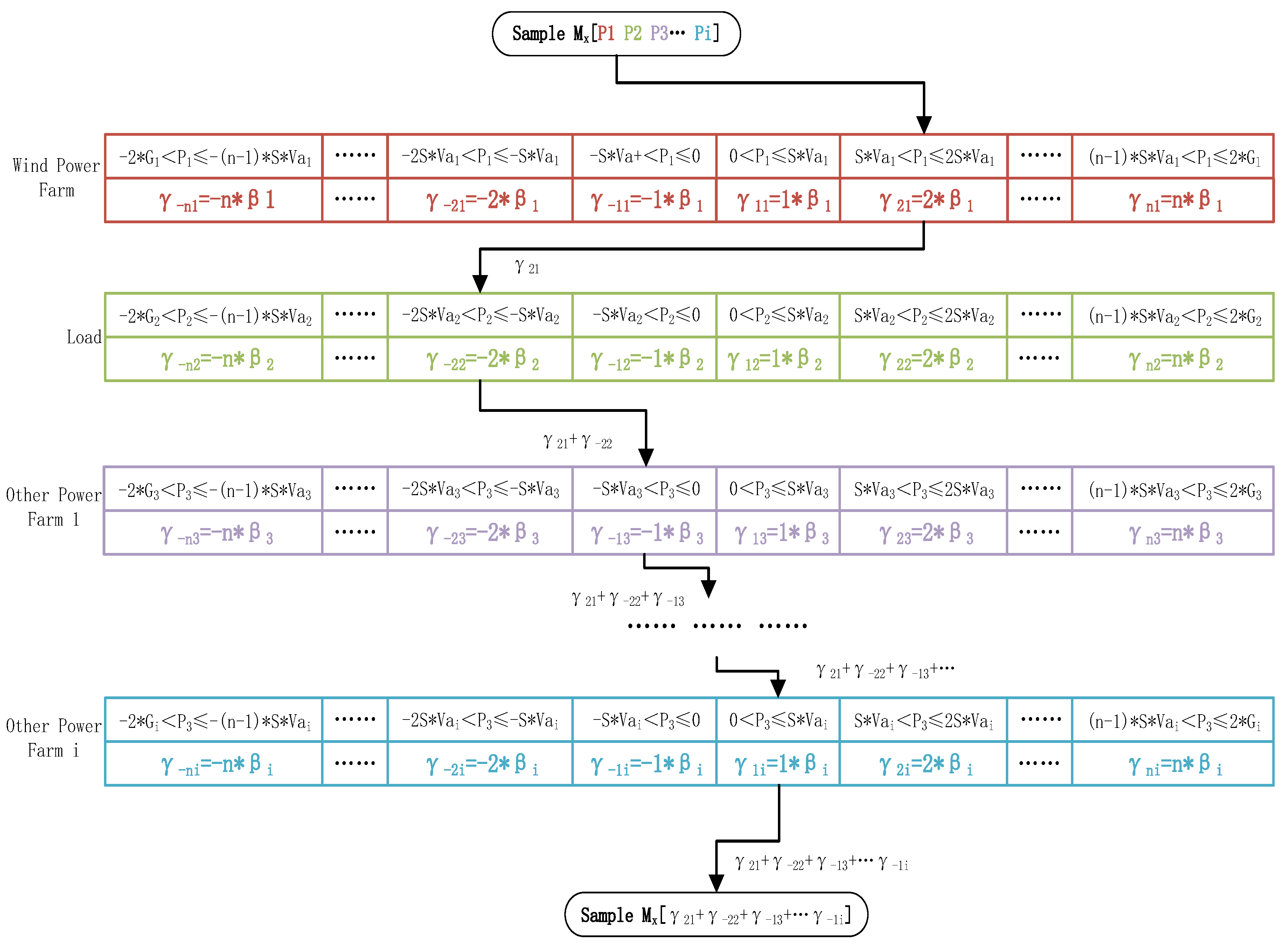
Based on the use of changing values to define wind power ramp events, this paper proposes a self-selected multi-layer coefficient correction model (CSMCC) shown in Figure 5. The CSMCC includes multiple layer structures, which contain $2*n$ channels. Each channel contains two parts, including the front-end channel selection standard and the back-end correction coefficient. The sample traverses each layer according to the front-end channel selection standard in each layer, and obtains the back-end correction coefficient of the channel for a cumulative correction. Finally, we use the final cumulative coefficient to determine the wind power ramp event.

We set the parameters of the CSMCC, according to the actual information of the power system. We set the model layer number $i$ according to the total number of objects described in the power system. We set the total number of described objects in the power system as $Num$. Then the model layer number $i$ is as shown in Formula (2).

$$i=Num$$

(2)

After selecting the wind power ramp threshold $Var$, we set the threshold amount ${\left[\begin{array}{ccccc}{G}_1& G_2& G_3& \cdots & G_i\end{array}\right]}^T$ according to the installed capacity ${\left[\begin{array}{cccc}Va1& Va2& \begin{array}{cc}Va3& \cdots \end{array}& Vai\end{array}\right]}^T$ of each described object in the power system, as shown in Formula (3).

$$\left[\begin{array}{c}Va1\\ Va2\\ Va3\\ ⋮\\ Vai\end{array}\right]=\left[\begin{array}{c}Var*G_1\\ Var*G_2\\ Var*G_3\\ ⋮\\ Var*G_i\end{array}\right]$$

(3)

We set the described coefficient ${\left[\begin{array}{cccc}{\alpha }_1& {\alpha }_2& \begin{array}{cc}{\alpha }_3& \cdots \end{array}& {\alpha }_i\end{array}\right]}^T$, according to the actual operation of each object in the power system, as shown in Formula (4).

$$\{\begin{array}{c}{\alpha }_i=1(\hspace{0.17em} i input active power to the grid\hspace{0.17em} )\\ {\alpha }_i=0(i outputactive power from the grid)\end{array}$$

(4)

We set the layer coefficient ${\left[\begin{array}{cccc}{\beta }_1& {\beta }_2& \begin{array}{cc}{\beta }_3& \cdots \end{array}& {\beta }_i\end{array}\right]}^T$ according to the described coefficient of each object and the installed capacity, as shown in Formula (5).

$$\left[\begin{array}{c}{\beta }_1\\ {\beta }_2\\ {\beta }_3\\ ⋮\\ {\beta }_i\end{array}\right]=\left[\begin{array}{c}{(-1)}^{{\alpha }_1-1}*G_1/(G_1+G_2+G_3+\cdots +G_i)\\ {(-1)}^{{\alpha }_2-1}*G_2/(G_1+G_2+G_3+\cdots +G_i)\\ {(-1)}^{{\alpha }_3-1}*G_3/(G_1+G_2+G_3+\cdots +G_i)\\ ⋮\\ {(-1)}^{{\alpha }_i-1}*G_i/(G_1+G_2+G_3+\cdots +G_i)\end{array}\right]$$

(5)

According to the described coefficient and installed capacity of each object, the total power plant installed capacity coefficient is obtained as shown in Formula (6).

$$Per=\frac{\left[\begin{array}{ccccc}{\alpha }_1& {\alpha }_2& {\alpha }_3& \cdots & {\alpha }_i\end{array}\right]{\left[\begin{array}{ccccc}{G}_1& G_2& G_3& \cdots & G_i\end{array}\right]}^T}{\left(G_1+G_2+G_3+\cdots +G_i\right)}$$

(6)

Considering the accuracy requirements of this model, we set the channel width to $S$, generally, $S$ is set to 0.1, and set the front-end channel selection criteria according to the threshold value ${\left[\begin{array}{cccc}Va1& Va2& \begin{array}{cc}Va3& \cdots \end{array}& Vai\end{array}\right]}^T$. Considering the actual situation of the power system, we set the upper limit of the channel to $2*G_i$ and the lower limit to $-2*G_i$, where each layer contains $2n$ channels, and the channel coefficient of each channel is $\left[\begin{array}{cccc}-n& -n+1& \begin{array}{cc}\begin{array}{ccc}\cdots & -1& 1\end{array}& \cdots \end{array}& \begin{array}{cc}n-1& n\end{array}\end{array}\right]$. The correction coefficient $\gamma$ at the back end of the channel is shown in Formula (7).

$$\gamma ={\left[\begin{array}{ccccc}{\beta }_1& {\beta }_2& {\beta }_3& \cdots & {\beta }_i\end{array}\right]}^T\left[\begin{array}{cccccccc}-n& -n+1& \cdots & -1& 1& \cdots & n-1& n\end{array}\right]$$

(7)

The CSMCC model is shown in Figure 5. Suppose $M_x$ is the No. x selected sample. P1 of sample $M_x$ satisfies the front-end selection standard of the ${\gamma }_{21}$ channel in a wind power farm layer, P2 of sample $M_x$ satisfies the front-end selection standard of the ${\gamma }_{-22}$ channel in the load layer, P3 of sample $M_x$ satisfies the front-end selection standard of the ${\gamma }_{-13}$ channel in the other power farm layer, Pi of sample $M_x$ satisfies the front-end selection standard of the ${\gamma }_{-1\mathrm{i}}$ channel in the other power farm layer. Through the process in Figure 5, the final correction coefficient $R$ can be obtained, as shown in Formula (8).

$$R={\gamma }_{21}+{\gamma }_{-22}+{\gamma }_{-13}+\cdots +{\gamma }_{-1i}$$

(8)

When the correction coefficient $R$ satisfies Formula (9), the ramp event is considered to occur in this period.

$$R>Per/S$$

(9)

The back-end correction coefficient in this model includes two parts: the channel coefficient and the layer coefficient. The acquisition of the channel coefficient is related to the threshold value and actual power change value of each described object. The acquisition of the layer coefficient is related to the nature of each described object in the power system. Therefore, the use of this model to identify wind power ramp events not only considers the nature of each described object in the power system, but also considers the mutual influence of each described object at each moment. The number of layers can be adaptively adjusted according to the number and nature of the actual described objects in the power system. Therefore, the model can identify wind power ramp events in the power systems in different regions and has strong universality.

3.2. Quantitative Selection Method of the Threshold Considering Grid Frequency

In current research, the most commonly used method is to directly select the percentage of the total installed capacity to set the threshold. However, this threshold setting method is not clearly defined and is based on experience. When a ramp event occurs, the imbalance of active power will definitely have a corresponding impact on the frequency of the power system. Thus, we come up with a selection method of the threshold, according to the allowable value of the power system frequency change.

In the power system, the change between frequency and power is mainly related to the primary frequency modulation and the secondary frequency modulation of the power system. The primary frequency modulation is the frequency modulation method that each generator participates in. It is mainly aimed at power changes with small change range, short cycle, and contingency. It is mainly aimed at power changes with a small change range, a short cycle, and contingency. The secondary frequency modulation is mainly realized by specific frequency modulation power farms, and is mainly aimed at power changes with large fluctuations, long periods, and impact.

Therefore, this paper uses the primary and secondary frequency modulation of the power system to set the threshold of wind power ramp events. It is considered as a wind power ramp event when the active power in the grid changes and the frequency still does not reach the range allowed of the grid after the primary frequency modulation of the grid, and a secondary frequency modulation is required.

The relationship between the amount of change in the active power of the power system and the amount of frequency change in the process of primary frequency modulation is shown below [10].

$$k\sigma =-\Delta f(\%)/\Delta P(\%)$$

(10)

In Formula (7), $\Delta f(\%)$ represents the percentage change of the power system frequency. $\Delta P(\%)$ represents the percentage change of the active power of the frequency modulation unit. $k\sigma$ represents the adjustment coefficient.

Further, we can get:

$$\Delta P(\%)=-\Delta f(\%)/k\sigma$$

(11)

We set $P_r$ to represent the total installed capacity of the power system, and wind power plants account for $n\%$ of the total installed capacity. According to the national power supply business rules [21], the allowable deviation of power supply frequency is 0.2 Hz when the total installed capacity of the power system is above 3 million kilowatts. The allowable deviation of power supply frequency is 0.5 Hz when the total installed capacity of the power system is below 3 million kilowatts. The adjustment coefficient $k\sigma$ is generally 4%~6%, the frequency requirement of the China power system is 50 Hz, and the percentage of the relative wind power ramp event threshold can be set as:

$$P_{val}=\alpha \ast (P_r\ast n\%)/(50\ast 6\%)$$

(12)

When the installed capacity of the sample is greater than 3 million kilowatts, $a=0.2$. When the installed capacity of the sample is less than 3 million kilowatts, $a=0.5$.

In order to show the effectiveness of the method proposed in this paper, we use the typical experience value selection threshold method in the literature for comparison and verification. This paper selects the data of two wind power farms to analyze the threshold selection method. Assuming that the maximum instantaneous power is the rated power, since the capacities of the two selected wind power farms are both less than 3 million kilowatts, α = 0.5. According to Formula (5), the selection of thresholds for two wind power plants can be obtained as shown in

Table 2. The selection of the threshold value of two wind farms.

Wind Farm	Literature [4] [kW]	Literature [22] [kW]	Literature [23] [kW]	Consider Grid Frequency [kW]
A	6661.57	27,756.57	11,102.61	9252.19
B	5430.60	22,627.50	9051.00	7542.50

. We divide the samples with the obtained thresholds, and obtain the proportion of samples with ramp events and the proportion of samples with no ramp events, as shown in Figure 6. Using the threshold quantitative selection method considering the grid frequency, the samples of ramp events in the two wind power farms accounted for 1.96% and 1.19% of the total, which is consistent with that described in the literature [12].

Although the calculation result of the threshold quantitative selection method considering the grid frequency is not very different from the traditional method of selecting the threshold based on empirical value, its interpretability and selection process formulation are clear advantages over the traditional threshold selection method. In addition, the threshold selection method considering the grid frequency and the CSMCC model are both from the perspective of the whole network operation, and the two methods have good compatibility.

In addition, the method of combining the CSMCC model and the threshold selection method considering the grid frequency to determine the ramp event can be adaptively changed, according to the change of the system operation mode. Although the installed capacity will not change in a short period of time, the system load, other renewable energy output, and the penetration level of wind power operation are constantly changing. Although the installed capacity will not change in a short period of time, the system load, other renewable energy output, and the penetration level of the wind power operation are constantly changing. In Figure 1, Figure 2, Figure 3 and Figure 4, the same wind power change can be judged as a “ramp” event in some operating modes, while it may be judged as a “no-ramp” event in other operating modes. Whether it is a ramp event or not depends on conditions such as wind power, load, other renewable energy output, and grid frequency. Therefore, the combination of the threshold quantitative selection method considering the grid frequency and the CSMCC model proposed in this paper is not only reasonable and feasible, but can also further reflect the ever-changing grid operation mode.

4. Result and Discussion

4.1. Practical Example Analysis of the Ramp Event Recognition

This paper selects the measured data with a sampling interval of 15 min in two local power systems in Inner Mongolia and Jilin (set as No. 1 and No. 2 power system), and analyzes actual calculation examples for the wind power ramp event identification method proposed in this paper.

Power systems 1 and 2, respectively, contain three parts: wind power farms, load, and photovoltaic power farms. We assume that the maximum instantaneous power is the rated power and select the threshold $Var$ according to Formula (6). At this time, the power system contains two parts: wind power output and photovoltaic power output. Therefore, $P_r$ in Formula (6) should be the total rated capacity of the wind turbine and photovoltaic generator.

We set the parameters of the CSMCC model according to the actual information of No. 1 and No. 2 power systems, as shown in

Table 3. Parameters of channel self-selection multi-layer coefficient correction model (CSMCC) in No. 1 and No. 2 power systems.

Parameter Name	Parameter Symbol	Parameter Value
Model layers	$i$	3
Threshold	${\left[\begin{array}{cccc}Va1& Va2& \begin{array}{cc}Va3& \cdots \end{array}& Vai\end{array}\right]}^T$	A: ${\left[\begin{array}{ccc}9252.2& 4298.2& 4174.7\end{array}\right]}^T$
		B: ${\left[\begin{array}{ccc}7542.5& 2865.4& 2783.8\end{array}\right]}^T$
Descriptive coefficient	${\left[\begin{array}{cccc}{\alpha }_1& {\alpha }_2& \begin{array}{cc}{\alpha }_3& \cdots \end{array}& {\alpha }_i\end{array}\right]}^T$	${\left[\begin{array}{ccc}1& 0& 1\end{array}\right]}^T$
Layer coefficient	${\left[\begin{array}{cccc}{\beta }_1& {\beta }_2& \begin{array}{cc}{\beta }_3& \cdots \end{array}& {\beta }_i\end{array}\right]}^T$	A: ${\left[\begin{array}{ccc}0.5220& 0.2425& 0.2355\end{array}\right]}^T$
		B: ${\left[\begin{array}{ccc}0.5718& 0.2172& 0.2110\end{array}\right]}^T$
Total power farm installed capacity coefficient	$Per$	A: 0.7575
		B: 0.7828
Channel width	$S$	0.1
Channel coefficient	$\left[\begin{array}{cccc}-n& -n+1& \begin{array}{cc}\begin{array}{ccc}\cdots & -1& 1\end{array}& \cdots \end{array}& \begin{array}{cc}n-1& n\end{array}\end{array}\right]$	$\left[\begin{array}{cccc}-240& -239& \begin{array}{cc}\begin{array}{ccc}\cdots & -1& 1\end{array}& \cdots \end{array}& \begin{array}{cc}239& 240\end{array}\end{array}\right]$

.

We use the CSMCC model to identify the ramp events in the No. 1 and No. 2 power systems. Part of the results of the ramp recognition on the No. 1 power system are shown in Figure 7 and

Table 4. The occurrence of wind power ramp events in grid 1.

Ramp Event	Ramp Event Period/15 min	Change of Wind Power/kW	Change of Load Side Power/kW	Change of Photovoltaic Power/kW
1	6–7	39,902.76	−110.26	0
2	7–8	−27,489.71	−316.55	0
3	16–17	17,797.73	308.45	−1184.19
4	22–23	−10,962.43	−318.97	−1140.80
4	33–34	15,940.97	−260.14	0
5	89–90	−44,356.50	126.37	0
6	94–95	15,706.47	31.89	3242.59
7	95–96	9037.76	80.06	11,897.79

.

In Figure 6, the red area is the wind power ramp event identified by the CSMCC model in the No. 1 power system, and the purple dotted line represents the wind power output ramp point. We can see that the main reason for the ramp samples of No. 1–3 and No. 5–7 is that the wind power output in the No. 1 power system has climbed during this period. In the No. 4 ramp event sample, although the wind power output has a significant downward trend, it does not reach the ramp threshold, which is not enough to cause the wind power ramp event. However, at this time, the photovoltaic power output in the No. 1 power system also has a significant decline. Under theinfluence of the wind farm and photovoltaic farm, the active power of the grid is unbalanced, which means the wind power ramp event occurs.

We use the CSMCC model to identify and analyze the ramp events in the No. 2 power system, and some of the results obtained are shown in Figure 8 and

Table 5. The occurrence of wind power ramp events in grid 2.

Ramp Event	Ramp Event Period/15 min	Change of Wind Power/kW	Change of Load Side Power/kW	Change of Photovoltaic Power/kW
1	3–4	−1205.79	64.35	−10,010.93
2	4–5	194.01	−23.04	10,010.93
3	8–9	−2002.49	−138.22	−8692.40
4	41–42	15,854.28	−33.67	0
5	42–43	−13,624.73	−19.89	0

.

From the recognition results of the CSMCC model of the No. 2 power system, it can be seen that a total of five periods are identified as wind power ramp events. The samples No. 4 and No. 5 are the ramp events caused by a large steep rise and fall in the wind power output. The wind power output of the No. 1–3 ramp event sample all changed slightly, and the value was far from the threshold standard. However, at these three moments, the photovoltaic power farm experienced clear steep drops, steep rises, and steep drops, which caused the imbalance of active power in the power system that has become the leading factor in the occurrence of the ramp event. At the 95–96 moment, the wind power output changed sharply, and neither the load-side power nor the photovoltaic power output showed clear fluctuations. However, the CSMCC model does not define these moments as ramp events, mainly because, when only the rated capacity of the wind turbine is considered, the change in the wind power output at 95–96 can cause the frequency deviation in the grid to exceed the allowable value. However, in actual operation, in addition to the wind power output, the B grid also has photovoltaic power output. Therefore, the total installed capacity of the grid becomes larger. The change of the wind power output at 95–96 times cannot cause the frequency deviation of the B grid to exceed the allowable value. No ramp event occurred at this point. In the method of quantitative selection of the threshold based on a grid frequency, $P_r$ is the total capacity of the grid, which changes with the actual operation of the grid. Therefore, in the B grid, $P_r$ is set as the sum of the rated capacity of wind turbines and photovoltaic power plants. Thereby, the threshold value in the CSMCC model is increased, so that the special situation in the 95–96 period is correctly identified.

From the recognition results of the ramp events of the No. 1 and No. 2 power systems, it can be seen that, compared with the traditional wind power ramp event recognition method, using the threshold quantitative selection method based on grid frequency and the CSMCC model, both the positive and negative peak shaving characteristics between the wind generator and the load can be considered. In addition, the complementary characteristics of the wind generator and other renewable energy power output in the power system can be considered. Therefore, from the perspective of the overall operation of the power system, the result of identifying the wind power ramp event is more accurate, and it has more practical significance for the operation and dispatch of the power system.

4.2. Predictability Analysis of a Described Object

On the basis of definition and identification, the wind power ramp forecast is carried out to comprehensively evaluate large-scale wind power ramp events, which is of great significance to the effective control of the wind power ramp. Generally, data-driven modeling is a commonly used forecasting method, which can mine and extract some relevant information existing in the time series. Therefore, it is necessary to study the correlation of the sequence [23].

Assuming that ${\left\{x_t\right\}}_{t=1:n}$ is a random time sequence, the autocorrelation coefficient between $x_t$ and its delay of $k$ steps $x_{t+k}$ represents the degree of correlation between the two signals. The larger the autocorrelation coefficient, the stronger the dependence between the two signals. Statistical methods can be used to dig out the laws hidden in the data to realize the prediction of future data.

There are many methods for time series autocorrelation analysis. Among them, the Pearson autocorrelation analysis method is a classic method. Its basic principles are as follows.

Assuming that ${\left\{x_t\right\}}_{t=1:n}$ is a random time series, the calculation formula for measuring the autocorrelation coefficient $\rho (k)$ between $x_t$ and its delay of $k$ steps $x_{t+k}$ is as follows.

$$\gamma (k)=cov(x_t,x_{t+k})=E[(x_t-\overline{x})(x_{t+k}-\overline{x})]$$

(13)

$$\rho (k)=\frac{\gamma (k)}{\gamma (0)}$$

(14)

In the actual calculation, $k$ is the delay step. $\overline{x}$ is the average value of the power time series in different characterization methods. $x_{t+k}$ is the time series obtained after delaying the original power time series $x_t$ by $k$ steps. $\gamma (k)$ is the covariance after delaying $k$ steps. $\gamma (0)$ is the covariance when the delay step $k=0$. $\rho (k)$ is the autocorrelation coefficient obtained after delaying $k$ steps. Analyze the predictability of wind power time series under different characterization methods according to the calculation results. Generally, the correlation coefficient and its corresponding degree of correlation are shown in

Table 6. Correlation coefficient with its dependence degree.

Relevance	Very Strong Correlation	Strong Correlation	Moderately Correlation	Weak Correlation
$\left|{\rho }_{xx}(\tau )\right|$	0.8~1.0	0.6~0.8	0.4~0.6	0.2~0.4

.

In the correlation analysis of this article, the sequence length with a correlation coefficient greater than 0.6 is selected as the predictable step size of this time sequence.

This paper selects the measured data of a local power system in Inner Mongolia (set as the No. 1 power system) with a sampling interval of 15 min. This paper first predicts the power of each described object and then uses the CSMCC model to identify wind power ramp events. We perform autocorrelation analysis on the above time series, and the results are shown in Figure 9. In the No. 1 power system, the length of wind power output autocorrelation of 0.6 or more is 300 min. The length of the load-side power autocorrelation of 0.6 or more is 47,400 min. The length of photovoltaic power output autocorrelation of 0.6 or more is 18,750 min. All of them meet the forecast conditions.

In order to verify the universality of the conclusions, another wind farm in Jilin Province was selected as the No. 2 power system for auto-correlation analysis. The results are shown in Figure 10. In the No. 2 power system, the length of the wind power output with autocorrelation of 0.6 is 315 min. The length of load-side power autocorrelation of more than 0.6 is 47,520 min. The length of photovoltaic power output of autocorrelation of more than 0.6 is 21,615 min in which all meet the prediction conditions.

To sum up, the photovoltaic power output and wind power output as well as load side power time series have a certain correlation. It is feasible to carry out data-driven modeling and forecasting for the photovoltaic power output and wind power output as well as load side power of the two wind farms based on the formation of a quantitative description method of ramp events. In order to verify the practical feasibility of the above definition and identification method, the forecast calculation example will be analyzed below.

4.3. Example Analysis of the Wind Power Ramp Event Prediction

This paper chooses the BP neural network and support vector machine to establish the prediction model. The first 1800 data of No. 1 power system is selected as the training set, and the last 100 data is selected as the test set. First, predict the power of each described object in the No. 1 power system, and then use the CSMCC model to identify the prediction results and determine the wind power ramp event. The power prediction situation of each object in the No. 1 power system is shown in Figure 11, Figure 12 and Figure 13.

In Figure 11, the error (NRMSE) of using the BP neural network to predict the wind power output is 0.1530. The error (NRMSE) of using SVM to predict the wind power output is 0.1482.

In Figure 12, the error of using the BP neural network to predict the load-side power (NRMSE) is 0.0025. The error of using SVM to predict the load-side power (NRMSE) is 0.0788. SVM shifted right when compared with BPNN. It may be because the actual value fluctuates less, so BPNN has a higher fitting degree. Since rolling prediction is used in this paper, SVM may rely more heavily on samples at the previous moment when the model is established. Therefore, the image looks like it shifted right.

In Figure 13, the error (NRMSE) of using the BP neural network to predict the photovoltaic power output is 0.1020. The error of using SVM to predict the photovoltaic power output (NRMSE) is 0.1096.

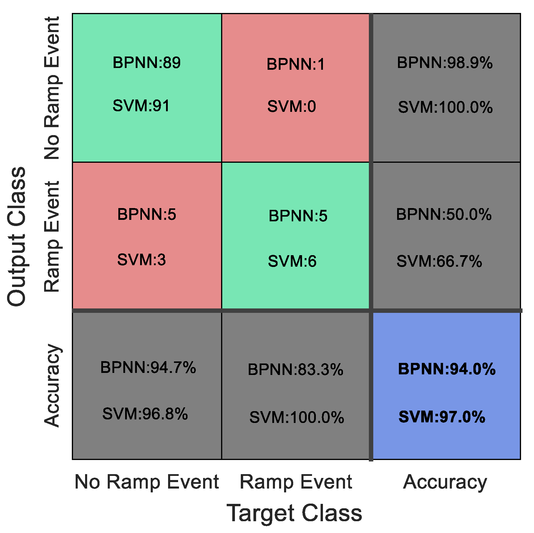
It can be seen that the prediction accuracy of each object in the No. 1 power system is better. After the prediction result is identified by the CSMCC model, the result of the analysis using the confusion matrix is shown in Figure 14.

In Figure 14, the green area represents the predicted value and the actual value are the same, and the red area represents the predicted value and the actual value are different. The two gray parts in the last row represent the prediction accuracy of no ramp event and the prediction accuracy of the ramp event, respectively. The blue area represents the overall forecast accuracy. It can be seen that, using the combination of the BP neural network, the support vector machine, and the CSMCC model to predict the No. 1 power system, the prediction accuracy of the “no-ramp” event is 94.7% while the prediction accuracy of the “ramp event” is 83.3%. The overall forecast accuracy rate is 94.0%. It can be seen from the prediction results that the wind power ramp event prediction method that uses the combination of the BP neural network, support vector machine, and CSMCC model to consider the generalized source-net-load information can achieve indirect prediction of wind power ramp events.

In order to verify the universality of the conclusions, the No. 2 power system was selected for the same data processing. The first 1800 data points are also selected as the training set, and the last 100 data points are selected as the test set. The predicted situation of each object in the power system is shown in Figure 15, Figure 16 and Figure 17.

In Figure 15, the error (NRMSE) of using a BP neural network to predict the wind power output is 0.1024. The error (NRMSE) of using SVM to predict the wind power output is 0.1030.

In Figure 16, the error of using a BP neural network to predict the load-side power (NRMSE) is 0.0053. The error (NRMSE) of using SVM to predict the load-side power is 0.0784.

In Figure 17, the error (NRMSE) of using a BP neural network to predict the photovoltaic power output is 0.1176. The error (NRMSE) of using SVM to predict the photovoltaic power output is 0.1322.

After using the CSMCC model to identify the prediction results, the results of the analysis using the confusion matrix are shown in Figure 18.

It can be seen from Figure 18 that using the combination of the BP neural network, support vector machine, and CSMCC model to predict the No. 2 power system, the prediction accuracy of the “no-ramp” event is 97.9% while the prediction accuracy of the “ramp” event is 80.0%. The overall prediction accuracy rate is 97.0%. From the analysis of the prediction results of the two wind farms, it can be seen that the accuracy of the indirect prediction using the combination of the BP neural network, support vector machine, and CSMCC model for both the sample points of “ramp” events or “non-ramp” events meets the forecast. Therefore, the wind power ramp event prediction method that uses the combination of the BP neural network, the support vector machine, and the CSMCC model to consider generalized source-net-load information can realize an indirect prediction of wind power ramp events.

5. Conclusions

Large fluctuations in power within a short period of time are prone to wind power ramp events. This paper studies the comprehensive evaluation method of wind power ramp events combined with generalized source-grid-load information, and the conclusions are as follows.

• A self-selected multi-layer coefficient correction model is proposed. In the identification of the wind power ramp time, the source side and load side information of the power system are comprehensively considered, and the feasibility of the model is verified by examples.
• Combining the grid frequency to determine the threshold of a wind power ramp-up event, and giving a quantitative evaluation method for different grid capacities, using actual wind power plant data to demonstrate its rationality.
• Discussed the necessity of autocorrelation analysis in data-driven modeling and forecasting. The actual wind power plant data analysis results show that each description object in the power system has a relative length, and the time series based on data-driven modeling forecast results have a certain degree of reliability.

Using a BP neural network and support vector machine to analyze prediction examples, the prediction results have certain accuracy and credibility, which verifies that the comprehensive evaluation method proposed in this paper is feasible in practice.

This article is a preliminary study of the comprehensive evaluation method of wind power ramp events combined with generalized source-grid-load information, which is of great significance for the comprehensive evaluation and early warning control of large-scale wind power ramp events. On this basis, further studies will be conducted on the temporal and spatial distribution characteristics of wind power ramp events, accurate forecasting, and deeper issues.