Short-Term Load Forecasting Algorithm Using a Similar Day Selection Method Based on Reinforcement Learning

Abstract

Short-term load forecasting (STLF) is very important for planning and operating power systems and markets. Various algorithms have been developed for STLF. However, numerous utilities still apply additional correction processes, which depend on experienced professionals. In this study, an STLF algorithm that uses a similar day selection method based on reinforcement learning is proposed to substitute the dependence on an expert’s experience. The proposed algorithm consists of the selection of similar days, which is based on the reinforcement algorithm, and the STLF, which is based on an artificial neural network. The proposed similar day selection model based on the reinforcement learning algorithm is developed based on the Deep Q-Network technique, which is a value-based reinforcement learning algorithm. The proposed similar day selection model and load forecasting model are tested using the measured load and meteorological data for Korea. The proposed algorithm shows an improvement accuracy of load forecasting over previous algorithms. The proposed STLF algorithm is expected to improve the predictive accuracy of STLF because it can be applied in a complementary manner along with other load forecasting algorithms.

1. Introduction

One of the main research topics in power engineering is short-term load forecasting (STLF), which consists of predicting the demand for an electrical load within a few hours or days. Improving the accuracy of STLF is important for the stability, safety, and efficiency of a power system. This is because STLF affects the power market and the planning and operations of the power plants in a power system [1,2]. In particular, the supply capacity of small photovoltaic (PV) power generators has increased in recent years. The increment in PV power generation has increased the uncertainty of load change, thereby making it increasingly difficult to predict the power demand. In recent years, numerous researchers have studied the improvement in the accuracy of STLF to address this problem.

Conventionally, STLF has been mainly used as a time series predictive model [3,4,5,6,7,8,9] that is based on the trend of the load changes in historical data and as a regressive prediction model [10,11,12,13,14] based on the relationship between the load and external variables such as weather [15]. However, conventional predictive models have the limitation that they do not reflect the nonlinear behavior in recent load trends [16]. To overcome these limitations, various forecasting methods such as fuzzy logic [17], fuzzy neural networks [18], particle swarm optimization [19], and support vector machines [20,21] were proposed. These methods can reflect the nonlinear behavior of the load. In particular, various forecasting models based on artificial neural networks (ANNs) have been primarily used [22]. The load forecasting models based on ANNs are being investigated in a variety of environments, and they are applied in a number of utilities that perform load forecasting with high accuracy.

Most load forecasting models set the load as an output variable and describe the quantitative relationship between the load and external variables. In contrast, the STLF method that uses similar days is based on finding a load that is similar to the load of the past and the forecasted target day [23]. Typically, the STLF method based on a similar day predicts the load of the target day by using the load of a similar day and external factors [15]. Even though the key advantage of the STLF method is that it is highly intuitive, it is considerably difficult to create a mathematical rule in terms of selecting similar days from the data for nonlinear external variables and the effect of nonlinearities. Thus, in most utilities, additional corrections by an experienced professional operator are still used along with the STLF algorithm based on similar days.

This study proposes the concept of applying the reinforcement learning algorithm, which is an artificial intelligence technique, to select a similar day. The STLF algorithm that uses similar days is based on the backpropagation neural network (BPNN) model. In recent years, studies have attempted to apply the reinforcement learning algorithm in load forecasting. The representative case is the study of the selection algorithms for the optimal model of load forecasting [24,25]. A reinforcement learning-based control method for occupant comfort in buildings was studied from an energy perspective [26]. In addition, studies in the field of energy and demand response have rapidly increased since the publication of the paper “Playing Atari with Deep Reinforcement Learning” in 2015. Most of these studies are related to the control of electric vehicles, batteries, heating, ventilation, and air conditioning (HVAC) systems, and no studies related to load forecasting have hitherto been reported [27].

The reinforcement learning algorithm is one of the most representative machine learning techniques along with supervised learning and unsupervised learning. After 2013, the Deep Q-Network (DQN) method was proposed by DeepMind. The DQN method has been used in numerous studies in a variety of fields. Reinforcement learning is mainly applied to areas such as robot control, stock trading, resource allocation, recommendation systems, and natural language processing. Additionally, reinforcement learning is known to exhibit a good performance in making the optimal selection under given conditions [28]. Reinforcement learning is divided into value-based learning, which is represented by Q-learning, SARSA, DQN, and policy-based learning, which is represented by deep deterministic policy gradient (DDPG), advantage actor critic (A2C), asynchronous advantage actor critic (A3C), and proximal policy optimization (PPO)s. In this study, the DQN method is used to train the agent policy.

The purpose of this study is to apply the reinforcement learning algorithm to mathematically solve the problem of similar day selection while matching the level of an experienced professional operator. In addition, this work proposes a high-accuracy STLF algorithm that used the selected similar day from the proposed similar day selection model. The proposed algorithm is compared with the commonly used similar day selection method based on the Euclidean distance. The performance of the proposed STLF algorithm is investigated by comparing it with the load forecasting algorithm that utilizes a long short-term memory (LSTM) layer [29]. The data used for testing and investigation include the power demand and weather data that were acquired in South Korea in 2018 by the Korea Power Exchange and Korea Meteorological Administration. The proposed method is expected to be used as a foundation to improve the accuracy of STLF in the future.

The rest of this paper is organized as follows: Section 2 presents the overall model structure of the STLF algorithm, which applies the proposed similar day selection. Section 3 presents a Markov decision process (MDP) and the equations utilized for selecting a similar day while using reinforcement learning. Section 4 describes the case studies of the similar day selection results and the 24-h prediction result obtained using the proposed algorithm. Finally, Section 5 summarizes the proposed algorithm and presents the conclusions and directions for future work.

2. Architecture of the Proposed Algorithm

The architecture of the proposed algorithm consists of the selection of similar days based on the reinforcement algorithm and STLF based on an ANN. The procedure of the proposed algorithm is subdivided into the learning procedure for the similar day selection model and the STLF model. Thereafter, the testing procedure selects similar days and predicts the short-term load using the trained models. The learning procedure for the two models is repeated during every timestep in the testing period to continuously reflect the trend of the load as the forecasting point changes. As described in a previous study [30] that uses reinforcement learning with the DQN method, the use of continuous data reduces the performance of the reinforcement algorithm agent. Therefore, the architecture of the proposed algorithm contains a separate memory control module that manages the memory of the data. Figure 1 shows the overall procedure of the proposed algorithm.

2.1. Similar Day Selection Model Based on Reinforcement Learning

The purpose of the similar day selection model is to find the date when the load is similar to the load of the forecasted target date by searching for previous dates. This similar load indicates the 24-h load in MW or the pattern of the 24-h load. It depends on how the load for the selected day is used in the forecasting model. The proposed load forecasting model uses the amount of load as input data. The load forecasting model that uses the similar date based on the pattern of the 24-h load will be studied in the future. The general load forecasting model based on a similar day starts with creating a similar day selection criterion. This criterion determines which dates from the past will be selected as similar dates based on the forecasting date. The criterion is created while considering the factors to be used and the calculations to be performed to determine the selected factors. Various studies have shown that calendar factors and meteorological factors are primarily used for selecting similar days. These factors are known to accurately represent load changes. The calendar factors generally include the distance between the forecasted date and past dates, the day of the week, and special days such as public holidays. In addition, the meteorological factors generally include temperature, sun irradiation, raindrops, humidity, wind speed, and sensory temperature. The meteorological factors are mostly continuous variables, whereas the calendar factors are discrete variables, except for the distance between the days. The discrete variables, such as the day of the week, cannot directly calculate the similarity between the dates that are expressed as scalar values. Therefore, the proposed model is designed by categorizing the calendar factors while excluding the distance between the dates.

The meteorological factors for the forecasting date are unknown because they occur in the future; hence, the predicted meteorological factors should be used. However, to avoid the prediction error in the meteorological factors, the actual values of the meteorological factors are used instead of the predicted values. The proposed similar day selection model is trained using the past date, and similar days are selected by utilizing the trained model. The proposed similar day selection model is founded by the reinforcement learning algorithm, which uses the state for the target day as input data and similar days as output data. Figure 2 illustrates the structure of the proposed similar day selection model, which consists of an environment, an agent, and replay memory. The details of the behavior and formulation of the similar day selection model are described in Section 3.

2.2. Similar Day Selection Model Based on the Euclidean Distance

Numerous previous studies have calculated the weighted Euclidean distance of the factors that affect the load to select similar days from previous days. Equation (1) uses the weighted Euclidean distance as a comparison method to investigate the performance of the proposed similar day selection model in the case studies:

$$WE{D}^{f.i}=\sqrt{w_1\Delta D^{f.i}{{}_{dd}}^2+w_2\Delta T^{f.i}{{}_{24}}^2+w_3\Delta S{I}^{f.i}{{}_{sum}}^2+w_4\Delta R^{f.i}{{}_{sum}}^2},$$

(1)

where $WED$ is the weighted Euclidean distance between the forecasted target day and past days; $f$ is the index of the forecasted target day; $i$ is the index of the past date; $\Delta D_{dd}$ is the distance of days between dates $f$ and $i$; $\Delta T_{24}$ is the Euclidean difference in the 24-h temperature; $\Delta S{I}_{sum}$ is the Euclidean difference in the 24-h sun irradiation; and $\Delta R_{sum}$ is the Euclidean difference in the 24-h raindrops. In addition, $w$ is the weight calculated through training from the past data, and it is approximated by minimizing the following cost function.

$$\begin{array}{c}\mathrm{Minimize}{\displaystyle {\displaystyle \sum }_{\mathrm{k}=1}^{\mathrm{n}}}{\left(y^{f.i}-f\left(x_{\mathrm{k}}, w\right)\right)}^2,\mathrm{k}\in \mathrm{K}\\ f\left(x_{\mathrm{k}}, w\right)=\alpha \times WE{D}^{f.i}+\beta \end{array}$$

(2)

where $y^{f.i}$ is a dependent variable that represents the difference between the loads of target date $f$ and past date $i$. Moreover, y(f) is calculated as the root mean square percent error [31] between the loads of the target date and past date, as given by Equation (3). $\alpha$ and $\beta$ are the independent variables for the slope and y-intercept, respectively. $\mathrm{K}$ represents the past data that are used to calculate the weight.

$$y^{f.i}=\frac{1}{24}\times {\sum }_{t=1}^{24}\sqrt{(\frac{l{d}_t^f-l{d}_t^i}{l{d}_t^f}{)}^2},$$

(3)

where $l{d}_t^f$ is the load of the target day at time $t$ and $l{d}_t^i$ is the load of past day $i$ at time $t$. Similar days are selected using the smallest days by calculating the weighted Euclidean distance (WED) of the past days for the forecasted date. In addition, the range of the past days strongly affects the selection of similar days. In this study, the range of the past days is determined through trial and error.

The Euclidean distance similarity (EDS) between the measured loads of the target day and past days is defined to evaluate the performance of a selection result. As the EDS approaches one, the load of the selected day becomes more similar to the load of the target day. Moreover, as the EDS approaches zero, the load of the selected day becomes more dissimilar to the load of the target day. The EDS can be determined through the following equation:

$$EDS=\frac{1}{1+\frac{1}{24}\times {\sum }_{t=1}^{24}\sqrt{(\frac{l{d}_t^f-l{d}_t^i}{l{d}_t^f}{)}^2}}.$$

(4)

2.3. STLF Model Based on the BPNN

The purpose of the STLF model is to accurately predict the load of the target day. The input values of the proposed STLF model are the 24-h load and the meteorological factors of the selected days obtained using the similar day selection model. Here, temperature, sun irradiation, and raindrops are used as the meteorological factors. The output is the 24-h load for the target day. The BPNN is based on repetitive processes for calculating the gradient of the error in the backpropagation algorithm and a signal that is transferred forward. The general BPNN model can be mathematically expressed by defining the network structure based on layers, input and output data, activation functions, and other parameters to train the model. The network structure of the proposed BPNN model features a typical feedforward architecture with an input layer, a hidden layer, and an output layer, as shown in Figure 3 [32].

The input variables, $X_n$, in the input layer of the proposed BPNN model include the 24-h load and the meteorological factors for the selected similar days. The output variable, $Y_m$, in the output layer of the proposed BPNN model is the 24-h load for the target day. In the proposed STLF model, the input layer and output layer use the sigmoid function as the activation function and the output layer is linearly activated. The generalized delta rule is used to train the weight of the model [33].

2.4. STLF Model Based on Long Short-Term Memory

The STLF model with an LSTM layer is used for comparison in the case studies. This model uses the load of recent days, the meteorological factors of recent days and the target day as the input variables. In addition, the 24-h load for the target day is the output variable. Figure 4 presents the structure of the STLF model based on LSTM [29].

The normalized historical data consist of the day index, $\mathrm{D}$, the time index, $\mathrm{H}$, the temperature, $\mathrm{T}$, for the day index, and the load, $\mathrm{L}$, over the past few days. In addition, the normalized prediction data consist of the day index, $\mathrm{PD}$, the time index, $\mathrm{PH}$, and the temperature, $\mathrm{PT}$, for the target day. The hyperparameter of this model is created using trial and error, which is the same as the proposed algorithm. The details of the STLF algorithm based on the LSTM method are published in another paper [29].

3. Methodology of Proposed Similar Day Selection Method

The application of the reinforcement learning algorithm to solve a problem in the real world starts with the mathematical definition of the problem. This mathematical expression is the same as the expression of the MDP, and it can be expressed by state, action, reward, and cost functions in the finite MDP problem [34]. Furthermore, the interaction between the agent and environment should be defined. In addition, the Q-function to explain the action of the agent and the learning method with the corresponding data should be presented.

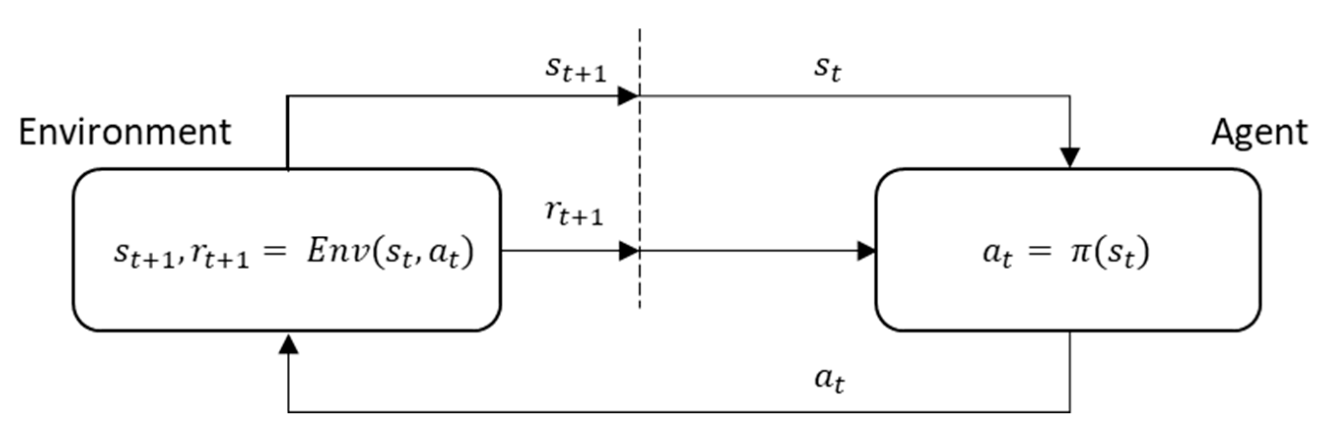
The reinforcement learning algorithm can be explained as the discrete stochastic version of the optimal control problem [34]. This implies that an optimal selection should be made through the interactions that occur at the sequential timesteps in a particular timeline. If this reinforcement learning algorithm is applied to the problem of similar day selection, it can be described as the problem of selecting the best similar day for STLF whenever the target day changes. This interaction is performed between the agent, which is subject to action, and the environment that responds according to the action. For timestep $t$, the agent selects action $A_t$ according to the observed state $S_t$ from the environment, and then, the action $A_t$ is forwarded to the environment. The environment communicates changed status $S_{t+1}$ along with prospective reward $R_{t+1}$ by reacting to action $A_t$. This continuously repeated process is referred to as agent–environment interaction, which is demonstrated in Figure 5.

In these repetitive interactions, the agent has a rule that determines the action to be performed depending on the observed state, and this rule is referred to as a policy. If the policy of the agent always makes the best selection for the expected cumulative reward for the future, then the policy can be assumed to be optimal. Thus, to mathematically represent the reinforcement learning algorithm, the state, action, and rewards must be defined according to the problem. Subsequently, the agent–environment interactions and the learning method of the policy of the agent should be designed.

3.1. Formulation of the Reinforcement Learning Algorithm

As previously described, the input variables for the similar day selection model use the calendar and meteorological factors. The purpose of the similar day selection model is to select the most similar date for the EDS, which can be calculated using Equation (4). From the agent’s perspective, the policy selects a specific date wherein the EDS is the highest, which is available for only the observation range. The observable states for the agent are the load, the calendar factors, the meteorological factors of the past days, and the action of selecting one of the past days as a similar day. Assuming that the target day changes for each timestep, the agent should be designed to perform the action of selecting a similar day that is based on the historical information for each target day.

The environment should output the reward at timestep $t$ and the state at timestep $t+1$ according to the action of the agent performed at timestep $t$. The reward at timestep $t$ is obtained by calculating the EDS of the load between the target day and similar days, which is determined by the action of the agent at timestep $t$. In addition, the state at timestep t + 1 is designed to be the state by moving the forecasted target day by one day.

The interaction between the environment and agent is reliable, as demonstrated in Equation (5), where $S$ is the universal set of the state, which is one of the environment’s output variables, $S_t$ is the state at timestep $t$, which is an element of $S$. $A$ is the universal set of the action determined by the agent, $A_t$. This is the action at timestep $t$, which is an element of $A$.

$$\begin{array}{c}{A}_t=agent\left(S_t\right)\\ R_t, S_{t+1}=environment\left(S_t,A_t\right)\end{array}$$

(5)

State $S_t$ is determined by the historical data that the agent can observe for each timestep. Assuming that the number of elements of the state is M and the number of observation days of the agent is N at timestep $t$, state $S_t$ can be determined from Equation (6) as follows:

$$\begin{array}{c}\mathrm{S}=\left[\begin{array}{ccc}{s}_{11}& \cdots & s_{m1}\\ ⋮& \ddots & ⋮\\ s_{1n}& \cdots & s_{mn}\end{array}\right]\\ s_{1n}=\left\{s_{1n},\dots ,s_{mn}\right\}=\left\{\Delta D^{f.n}{}_{dd},\Delta T^{f.n}{}_{24},\Delta S{I}^{f.n}{}_{24},\Delta R^{f.n}{}_{24}\right\}\end{array}$$

(6)

where $f$ is the index of the target day, $n$ is the index of the past day, $m$ is the index of the elements of the state, $\Delta D^{f.n}{}_{dd}$ is the distance between target day $f$ and past day $n$, $\Delta T^{f.n}{}_{24}$ is the Euclidean distance between the 24-h temperature for target day $f$ and past day $n$, $\Delta S{I}^{f.n}{}_{24}$ is the Euclidean distance between the 24-h sun irradiation for target day $f$ and past day $n$, and $\Delta R^{f.n}{}_{24}$ is the Euclidean distance between the 24-h raindrops for target day $f$ and past day $n$. The meteorological factors contain 24 elements that consider the difference in time series characteristics; thus, the total number of elements, m, in one past day is 73. In addition, the observation range should be set depending on the target system. The observation range for the proposed algorithm is set to be 90 days, which includes the past 30 days and 60 days from the previous year. Therefore, the total number of states for the output variables of the environment during timestep $t$ is 6570 elements.

The agents for finding similar days are learned using historical data. In the process of learning using past days, the environment already knows the information of past data, such as the load and meteorological data. Thus, it is possible to calculate the similarity between the loads of the target day and selected similar days from the agent. The learning of the agent to find similar days is a deterministic environment because it is limited in scope according to the target day and uses historical data. Therefore, the status of step t does not depend on the decision of the agent. In addition, the environment only reads the state information according to the timestep $t$ of the sequence and forwards it to the agent. 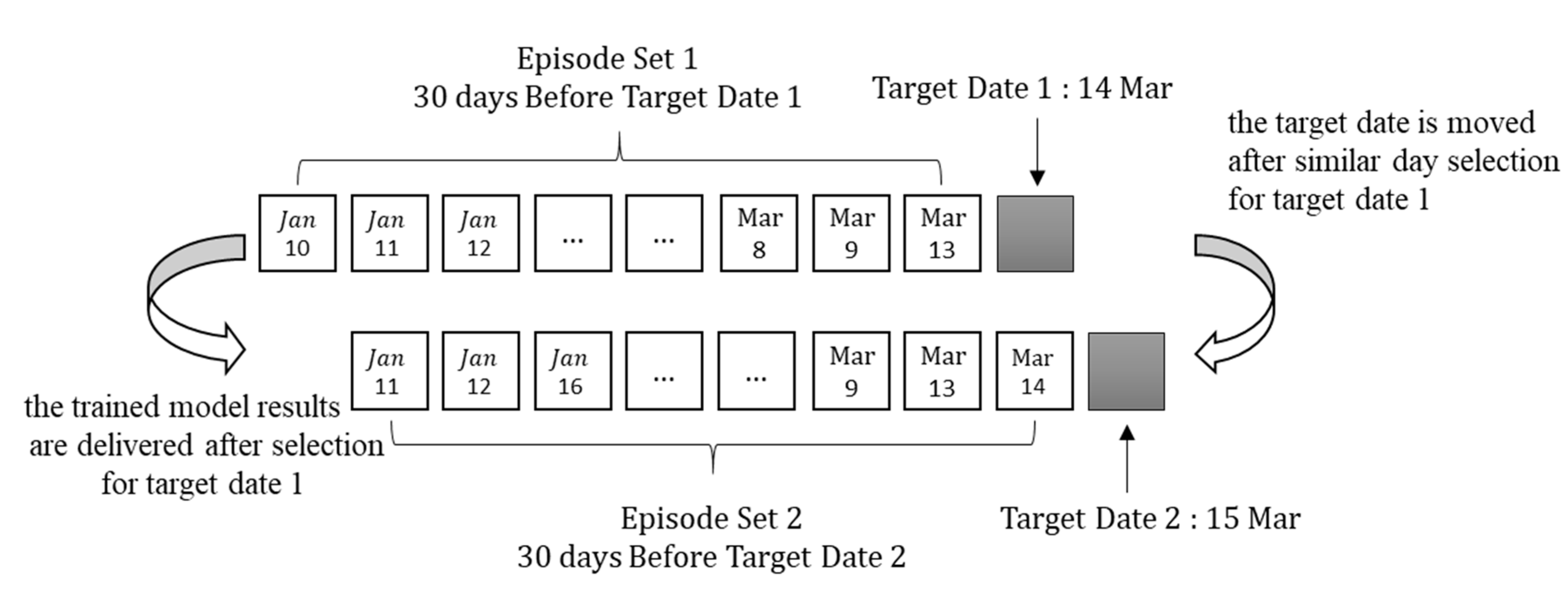Figure 6 illustrates the range of episodes according to the target date.

An episode is a period for learning the policy of the agent, which is expressed in the form of the DQN. In the example shown in Figure 5, if the target date is 14 March 2018, the initial timestep of the episode is 10 January 2018, which is 30 days before the target day, excluding special days. Furthermore, the terminal date is 13 March 2018. The agent receives the state information from the environment at each timestep. The state information comprises the calendar and meteorological factors of 90 days before each timestep. As the action of the agent in a deterministic environment does not affect the state transition, the state transition from the selected actions for similar days is not considered.

The number for the universal action set is the same as the observation range, $n$, and it can be expressed by the following equation:

$$\mathrm{A}=\left\{a_1, \cdots , a_n\right\}.$$

(7)

Here, element $a_n$ is a digit value, which implies that it is either zero or one. This indicates that a selected day can be expressed as one. One or more similar days can be selected depending on the manner in which they are used. The output of agent $A_t$ could consist of a number of combinations, ${\complement }_k^n$, depending on the number of selected days, $k$, according to the following equation:

$${\complement }_k^n=\frac{n!}{k!\left(n-k\right)!}.$$

(8)

A reward should be provided if the loads of the target day and selected days are similar and should not be provided if the loads are not similar. The EDS is calculated using the loads of the target day and selected days from Equation (4). In the proposed algorithm, the environment calculates the EDS from the past few days. A reward may or may not be provided, depending on whether a selected day is in the top three selected days.

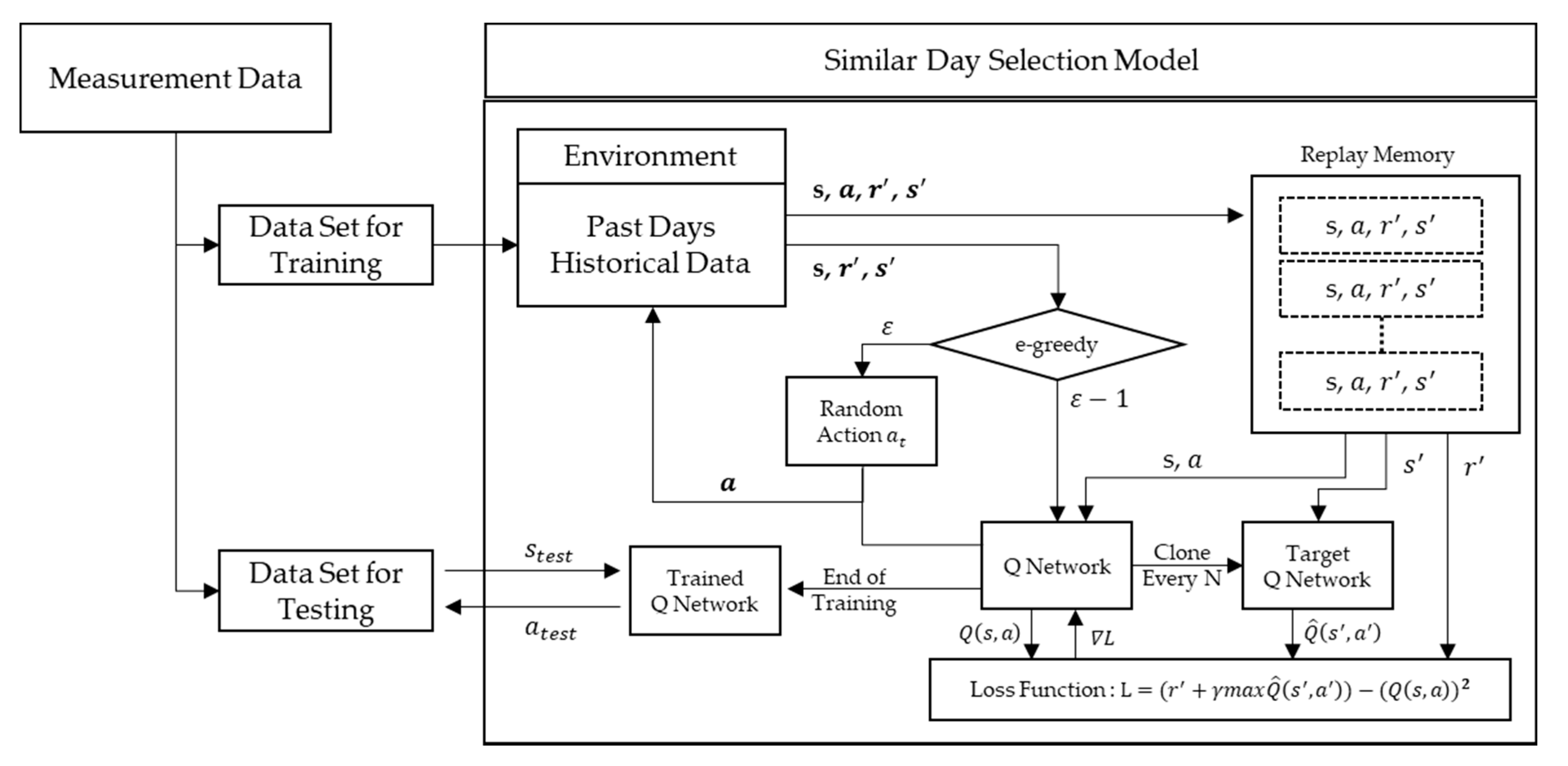
3.2. Deep Q-Network Training Algorithm

In this section, the DQN used to select a similar day is defined and an explanation is provided for the training method of the DQN. The proposed method is developed based on the DQN approach, among a number of different reinforcement methods. The DQN algorithm uses the Q-function as a state–action value function that can be approximated by the deep feedforward neural network structure [30]. The state–action value function expresses the expected cumulative reward, Q. This occurs when the agent selects action $A_t$ according to policy $\mathsf{\pi }$ in current state $S_t$. Policy π denotes a rule of the agent that determines which action to perform depending on the observed state. 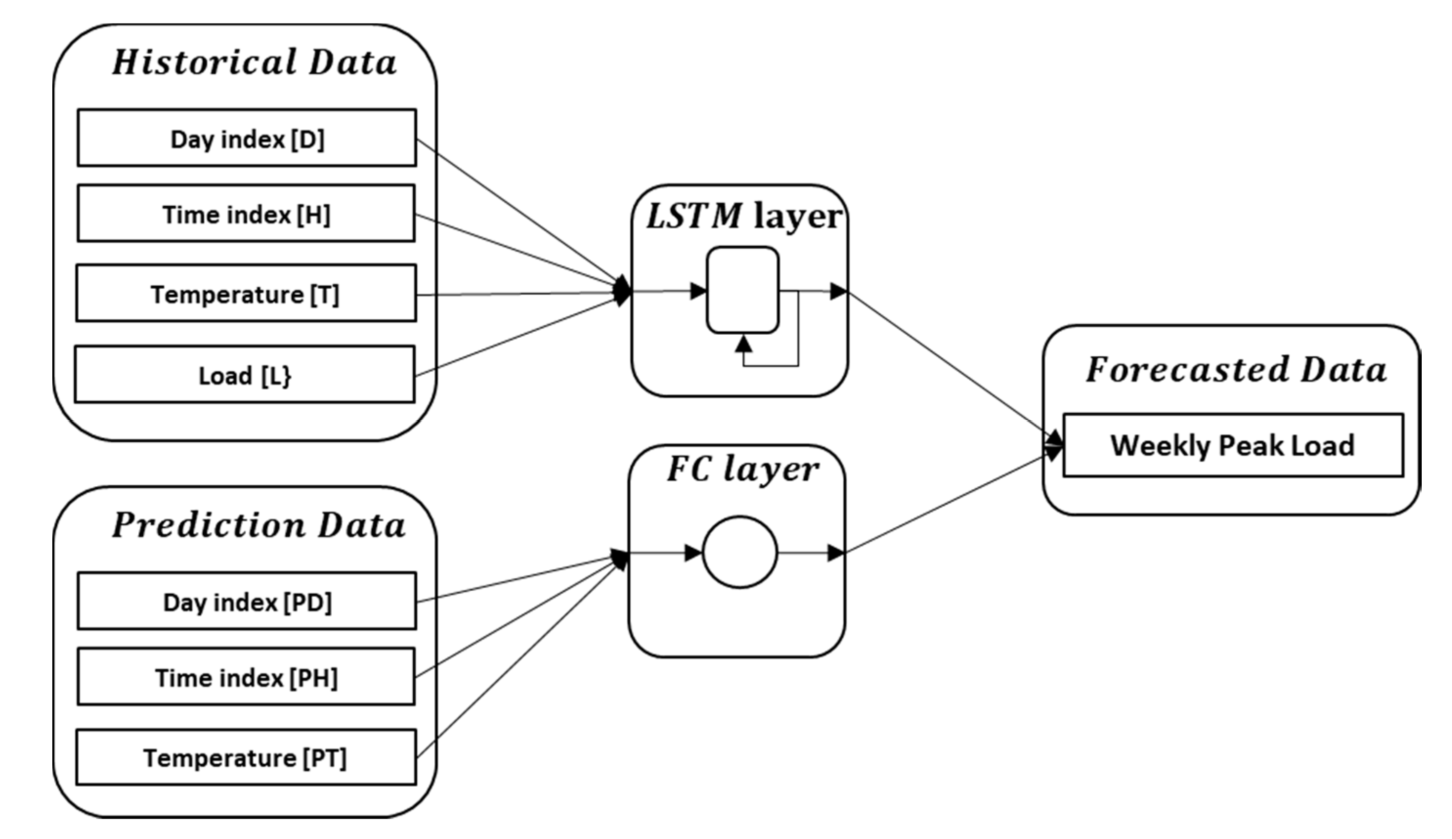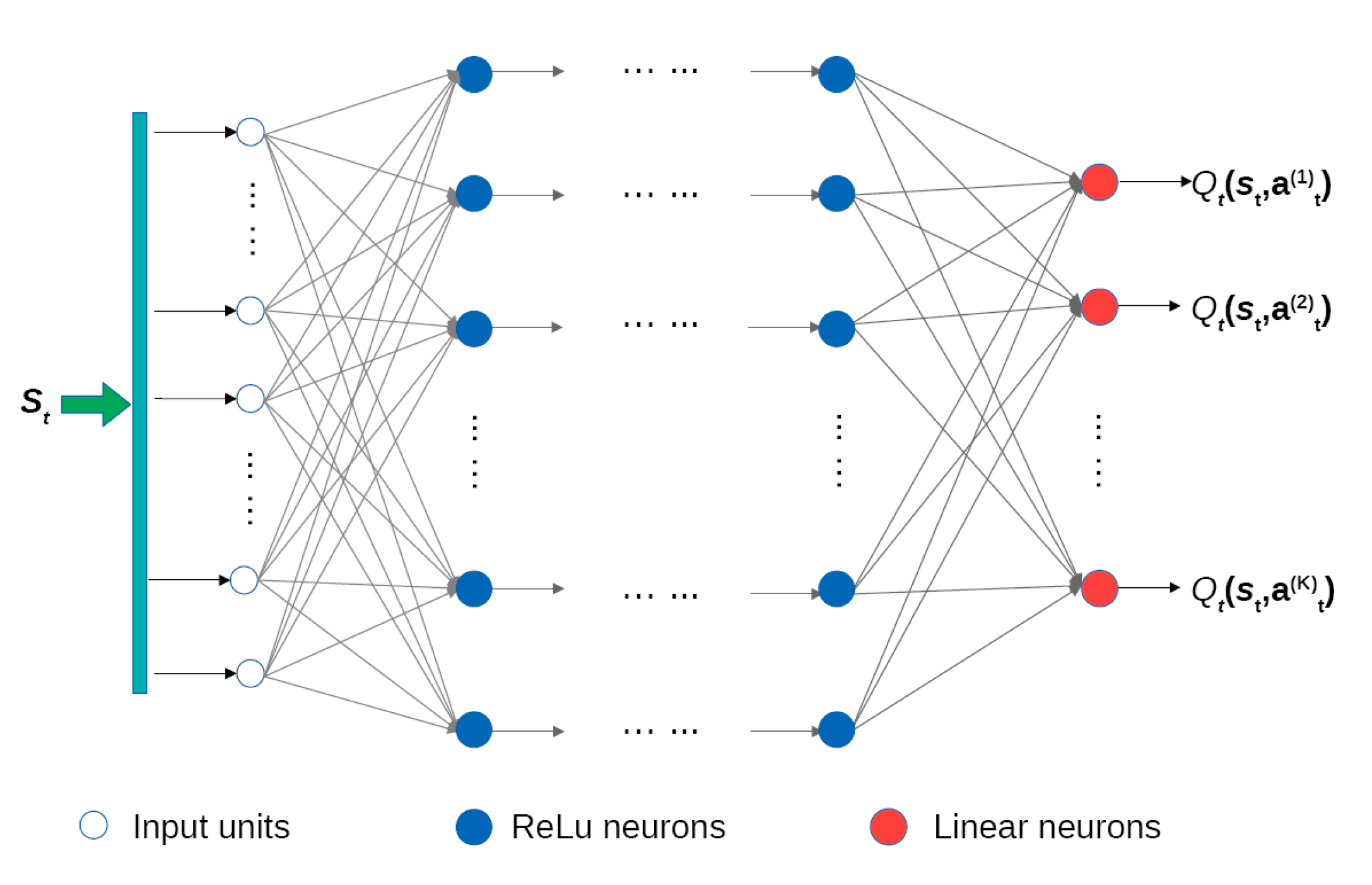Figure 7 illustrates the structure of the deep feed forward neural network used to express the expected cumulative reward, Q, according to action $A_t$ for state $S_t$.

The cumulative reward, $\mathrm{Q}\left(S_t,A_t\right)$, can be expressed by applying Equation (9) with the reward at the current timestep, $R_t$, and the expected reward at the next timestep, $\mathrm{Q}\left(S_{t+1},A_{t+1}\right)$.

$$\mathrm{Q}\left(S_t,A_t\right)=R_t+\mathrm{Q}\left(S_{t+1},A_{t+1}\right)$$

(9)

If the present value of the reward is higher than the reward expected in the future, Equation (9) can be expressed as Equation (10) by applying the discount factor:

$$\mathrm{Q}\left(S_t,A_t\right)=R_t+\mathsf{\gamma }\mathrm{Q}\left(S_{t+1},A_{t+1}\right)$$

(10)

If $\mathrm{Q}$ is expressed as $max\mathrm{Q}\left(S_{t+1},A_{t+1}\right)$ when selecting the action to maximize the expected cumulative reward at timestep $t+1$, Equation (10) can be expressed as Equation (11) using the Bellman Equation [34].

$$\mathrm{Q}\left(S_t,A_t\right)=R_t+\mathsf{\gamma }max\mathrm{Q}\left(S_{t+1},A_{t+1}\right)$$

(11)

By assuming that an optimal cumulative reward, $Q^{*}$, exists, $Q^{*}$, can be expressed as Equation (12):

$$Q^{*}\left(S_t,A_t\right)=R_t+\mathsf{\gamma }max{Q}^{*}\left(S_{t+1},A_{t+1}\right)$$

(12)

To make the random Q-function closer to the optimal Q-function through learning, the minimized loss function is defined as the difference between the Q-function and optimal Q-function. Loss function $\mathrm{L}$ can be determined using Equation (13):

$$\begin{array}{c}\mathrm{L}=Q^{*}\left(S_t,A_t\right)-\mathrm{Q}\left(S_t,A_t\right)\\ \mathrm{L}=R_t+\mathsf{\gamma }max{Q}^{*}\left(S_{t+1},A_{t+1}\right)-\mathrm{Q}\left(S_t,A_t\right)\end{array}$$

(13)

As the optimal Q-function is unknown, it is replaced with the target Q-function. The target Q-function uses the random variables at the beginning of training. Then, it is periodically replaced with the best Q-function that is found during the learning period. If the target Q-function is denoted as $\widehat{Q}$, the loss function can be expressed by Equation (14):

$$\mathrm{L}=R_t+\mathsf{\gamma }max\widehat{Q}\left(S_{t+1},A_{t+1}\right)-\mathrm{Q}\left(S_t,A_t\right)$$

(14)

The epsilon-greedy exploration method is used because it is not possible to find the value of an unexperienced action if the agent is operated by the Q-function. This is the agent that typically works with the Q-function; however, the agent selects a random action according to the probability of epsilon ε. The epsilon of the proposed algorithm starts with a value of 0.3, and then it converges to zero as the learning progresses.

The performance of the agent is reduced by performing repetitive learning with only highly relevant samples; hence, an experience replay method is used. This method is conceptually similar to a minibatch, which is a method of storing the previous history of samples in memory. Random samples are selected and used during the learning period. The pseudocode of the proposed DQN algorithm is as follows:

Algorithm 1. Q-network training algorithm for a similar day

Initialize: Replay memory D to capacity N

Initialize: Action Q-network $\mathrm{Q}$ with random weights $\mathsf{\theta }$

Initialize: Action Q-network $\widehat{Q}$ with random weights $\widehat{\mathsf{\theta }}$

for episode = 1, M do

observe initial state $S_t$ use formulation (5)

for t = 1, T do

select an action a

with probability $\mathsf{\epsilon }$ select a random action

else select action $A_t=\mathrm{argmaxQ}\left(S_t,A\right)$

observe $R_t$ and $S_{t+1}$ use formulation (4)

store experience <$S_t$, $A_t$, $R_t$, $S_{t+1}$> in replay memory D

sample random transitions <$S_j$, $A_j$, $R_j$, $S_{j+1}$> from D

set $y_j=\{\begin{array}{c}{R}_j, if episode terminates at step j+1\\ R_t+\gamma max\widehat{Q}\left(S_{t+1}, A_{t+1}\right), otherwise\end{array}$

train $\mathsf{\theta }$ using ${\left(y_j-\mathrm{Q}\left(S_j,A_j\right)\right)}^2$ as loss function

end for

update $\widehat{Q}=\mathrm{Q}$ every 20th step

end for

4. Case Studies

4.1. Data Description and Parameter Setting

The proposed algorithm is simulated using the measured load and meteorological data for Korea. All data used in the simulations are normalized to values ranging from zero to one to prevent the degradation of the predicted performance. The min-max normalization method is used, as shown in Equation (15):

$$X^{\prime }=\frac{X-X_{min}}{X_{max}-X_{min}}$$

(15)

$X^{\prime }$ is the value after normalization, $X$ is the original value, $X_{min}$ is the minimum value of the data in the observation range, and $X_{max}$ is the maximum value of the data in the observation range. The normalization criteria for the simulation data are shown in

Table 1. Normalization criteria for the simulation data.

Elements (Unit)	Maximum	Minimum
Load (MW)	100,000	0
Day Distance (Days)	700	0
Temperature (°C)	40	−40
Sun Radiation ($\mathrm{W}/{\mathrm{m}}^2$)	10	0
Raindrops ($\mathrm{mm}$)	100	0

.

The proposed algorithm consists of the similar day selection model and STLF model. Each model contains a separate neural network structure, and each neural network contains a separate hyperparameter. The hyperparameters of the similar day selection model consist of the number of hidden layers, the number of perceptrons, the buffer size, and the iteration number of an episode. The hyperparameters of the STLF model comprise the number of hidden layers, the number of perceptrons, and the learning rate. It is important to select the hyperparameters because they significantly impact the learning speed and performance. The hyperparameters are selected through trial and error in the simulation. The hyperparameters for each model are shown in

Table 2. Hyperparameters of the models for the case studies.

Model	Number of Hidden Layers	Number of Perceptrons	Size of the Buffer (N)	Iteration Number of Episodes (M)	Learning Rate (M)
Similar Selection Model	3	5000	1000	1000	0.001
Load Forecasting Model	2	1000	-	-	0.001

.

Data should be divided into training data and test data to evaluate the algorithms to solve prediction problems such as load forecasting. In this case study, the data for 32 days between March and April 2018 are used as the test data. The data for 30 days prior to the target day are used as the training data.

The historical total load of Korean power systems and the weather information for the Korean peninsula are used. The historical total load was provided by the Korea Power Exchange, which is the national service of the Republic of Korea. It controls the operation of Korea’s electricity market and power systems, the execution of real-time dispatch, and the establishment of the basic plan for supply and demand. The weather information was provided by the Korea Meteorological Administration, which is the national meteorological service of the Republic of Korea.

The Korean power systems had a supply capacity of 9957 MW and a peak load of 9247 MW in July 2018. The load composition was 55.7% for industrial load, 22.2% for commercial load, 13.9% for residential load, and the remaining 8.2% was used for other loads such as education and farming.

4.2. Performance of the Proposed Similar Day Selection Model

The performance of the similar day selection model is shown by calculating the EDS using Equation (4). As the EDS approaches one, the loads of the selected day and target day become more similar. Moreover, as the EDS value approaches zero, the loads of the selected day and target day become more dissimilar. The proposed similar day selection model improves the performance of the agent through repetitive learning. The agent calculates 32 rewards per episode. The initial agent is completely unlearned, and the proposed algorithm updates the parameters of the DQN for each iteration. To ensure that the DQN is learning as the episode progresses, the boxplot shown in Figure 8 groups the 320 rewards that are calculated during the 10 episodes. In addition, Figure 9 presents the average similarities between the loads of the selected days and target day, obtained using the DQN that is learned in each episode.

Figure 8 shows that the reward approaches 0.97 as the episodes progress. Figure 9 shows that the similar day selection performance between 6 March to 9 March improves in training. This implies that the similar day selection model works as expected. It is hypothesized that the similar day selection model can work for other test days as well.

Next, we compare the performance of the proposed similar day selection model and WED model. The EDS of the proposed model and WED model cannot be one because there is no past day that has the same load as the target day. Thus, the EDS is presented when the least similar date is selected, which is assumed using the optimal model. This implies that when the outputs of the proposed model and WED model are the same as that of the optimal model, the model selects the best similar day. Therefore, the performance of the optimal model is the criterion for evaluating the performance of the proposed model and WED model. The previous week (PW) model, which selects the same day of the previous week, is compared with the proposed model. The accuracy of the PW model is relatively low because it always selects the same day of the previous week as the due date.

With March 14 as an example date,

Table 3. Selected days and the Euclidean distance similarity (EDS) results of the models on 14 March 2018.

Selected Days	Optimal Model		RL Model		WED Model		PW Model
	Date	EDS	Date	EDS	Date	EDS	Date	EDS
Selected Day 1	2017-03-30	0.9935	2017-03-29	0.9805	2018-03-13	0.9751	2018-03-07	0.9171
Selected Day 2	2017-03-24	0.9872	2017-03-24	0.9872	2017-03-29	0.9805
Selected Day 3	2017-03-22	0.9868	2017-03-23	0.9856	2018-03-07	0.9171
Average		0.9892		0.9844		0.9576

shows the selected days that utilize the EDS when using the proposed reinforcement learning (RL) model, WED model, PW model, and optimal model. The average performances of the optimal model, RL model, PW model, and WED model on 14 March are 0.9892, 0.9844, 0.9171, and 0.9576, respectively. A comparison of the similar day selection performance of the models during March and April 2018 is presented in Figure 10, Figure 11,

Table 4. Similar day selection performance results in March and April 2018.

Month	Euclidean Distance Similarity
	Optimal Model	PW Model	WED Model	RL Model
1st week of March	0.9851	0.9123	0.9138	0.9650
2nd week of March	0.9704	0.9181	0.9473	0.9572
3rd week of March	0.9866	0.9413	0.9655	0.9766
4th week of March	0.9811	0.9444	0.9602	0.9757
1st week of April	0.9862	0.9598	0.9557	0.9699
2nd week of April	0.9823	0.9353	0.9628	0.9790
3rd week of April	0.9868	0.9682	0.9622	0.9736
4th week of April	0.9853	0.9673	0.9700	0.9783
Total Average	0.9833	0.9436	0.9546	0.9719

, and

Table 5. Similar day selection performance results by the day of week.

Day of Week	Euclidean Distance Similarity
	Optimal Model	PW Model	WED Model	RL Model
Monday	0.9828	0.9541	0.9570	0.9711
Tuesday	0.9790	0.9530	0.9583	0.9692
Wednesday	0.9770	0.9476	0.9499	0.9636
Thursday	0.9792	0.9429	0.9527	0.9683
Friday	0.9789	0.9426	0.9551	0.9701
Saturday	0.9799	0.9478	0.9563	0.9655
Sunday	0.9777	0.9508	0.9581	0.9646

. For the entire simulation period, the similarity is 0.9833 when the optimal days are selected, whereas it is 0.9719 and 0.9546 for the RL model and WED model, respectively.

4.3. Performance of the Proposed STLF Model

The accuracy of the proposed STLF model is compared with that of two models. The proposed model is a BPNN-based STLF model that uses the similar days selected by the proposed RL model (RL-BPNN model). The first model for comparison is a BPNN-based STLF model that uses the similar days selected by the WED model (WED-BPNN model). The second model for comparison is an LSTM-based STLF model (LSTM model) that is referenced in a previous study [29].

The accuracy of the STLF model is shown by calculating the mean absolute percentage error (MAPE) of the measured load and the forecasted load by each model, according to the following equation [36]:

$$\mathrm{MAPE}(\%)=\frac{1}{24}{\displaystyle \sum }_{t=1}^{24}\left|\frac{L_t^{measured}-L_t^{forecast}}{L_t^{measured}}\right|\times 100$$

(16)

The simulation uses 58 days in March and April 2018, except special days, as test data, which is the same as the test data set for the similar day selection model cases. The training period for each model is 30 days prior to the test day. Figure 12, Figure 13,

Table 6. MAPE of the models during March and April 2018.

Month	MAPE [%]
	RL_BPNN Model	LSTM Model	WED_BPNN Model
March	1.5133	1.8339	2.9937
April	1.1754	1.2363	1.9720
Average	1.3444	1.5351	2.4829

, and

Table 7. MAPE of the models by day of week.

Day	MAPE (%)
	RL_BPNN Model	LSTM Model	WED_BPNN Model
Monday	1.5295	1.5238	2.4172
Tuesday	1.2087	2.0282	2.4494
Wednesday	1.1524	1.1629	2.0219
Thursday	1.1854	1.7220	1.9567
Friday	0.9354	0.9625	2.3526
Saturday	1.8035	1.8046	3.2950
Sunday	1.5167	1.5109	2.7521

compare the MAPEs of the models for each day during the entire simulation period. In addition, Figure 14 shows a boxplot for the comparison of the general performance of the models.

It is confirmed that the proposed RL-BPNN model outperforms the other two models in terms of the average and maximum MAPE for the entire duration of the simulation. The average MAPEs of the loads forecasted by the proposed RL-BPNN model, WED-BPNN model, and LSTM model are 1.3444%, 2.4829%, and 1.5351%, respectively. The accuracy of the proposed model is 0.1907% higher than that of the LSTM model. In particular, the LSTM model reflects the time series characteristics of recent data; hence, the prediction error of the LSTM model increases intermittently. In contrast, the proposed RL-BPNN model is based on the similarity of the historical load data. As a result, the outlier is relatively small and the prediction error shows a continuous tendency. As there are advantages and disadvantages to each model, it would be better to use two algorithms in a complementary manner rather than using a single algorithm. In particular, the complementary forecasting methods that use the proposed method, such as the ensemble model, can contribute towards improving the predictive accuracy of STLF.

5. Conclusions

This work proposed an algorithm that uses a similar day selection model that is based on reinforcement learning and a load forecasting model, based on a BPNN that uses similar days. The proposed similar day selection model was developed based on the DQN technique. In addition, an MDP, environment, and agent were defined to develop a similar day selection model based on reinforcement learning. The proposed similar day selection model and the load forecasting model were tested using the measured load and meteorological data for Korea. The results of the case studies showed that the proposed method improved accuracy. That is, the proposed similar day selection model could determine the day that exhibited similar loads (97.19%), which was an improvement of 1.73% over the WED model. Moreover, the average MAPE of the proposed load forecasting model was 1.3444%, which was an improvement of 0.1907% in accuracy over the LSTM model.

The proposed similar day selection model does not require an environment-dependent weight learning process, unlike the widely used weighted Euclidean-based method. Therefore, the proposed model is expected to be highly capable of responding to environmental changes such as seasonal variations. Moreover, the parameters of the proposed model can be adjusted to maximize rewards through repetitive learning, so that it is possible to maintain the selection performance while considering the changes in the load over time. In particular, the proposed algorithm based on reinforcement learning can eliminate the dependence on an expert’s experience. Therefore, it is expected that the accuracy of STLF can be improved by applying the proposed algorithm along with other load forecasting algorithms via techniques such as the ensemble model.

Future research should address the quantification of the manner in which reinforcement learning models adapt to varying conditions. Furthermore, the similar day approach should be employed to conduct research on various artificial neural network models. Finally, research on improving the performance with regard to selecting the similar days should be performed by applying various model-based and model-free reinforcement learning techniques and selecting the similar days using a multi-agent system. Finally, the implementation of the STLF method using similar day selection models should be addressed.

References

1. Shahidehpour, M.; Yamin, H.; Li, Z. Market Operations in Electric Power Systems Forecasting, Scheduling, and Risk Management; John Wiley & Sons: New York, NY, USA, 2003; ISBN 978-0-471-46394-8. [Google Scholar]
2. Douglas, A.P.; Breipohl, A.M.; Lee, F.N.; Adapa, R. Risk due to load forecast uncertainty in short term power system planning. IEEE Trans. Power Syst. 1998, 13, 1493–1499. [Google Scholar] [CrossRef]
3. Amjady, N. Short-term hourly load forecasting using time-series modeling with peak load estimation capability. IEEE Trans. Power Syst. 2001, 16, 498–505. [Google Scholar] [CrossRef]
4. Hoffman, A.J. Peak demand control in commercial buildings with target peak adjustment based on load forecasting. In Proceedings of the 1998 IEEE International Conference on Control Applications (Cat. No. 98CH36104), Trieste, Italy, 4 September 1998; Volume 2, pp. 1292–1296. [Google Scholar]
5. Gonzales Chavez, S.; Xiberta Bernat, J.; Llaneza Coalla, H. Forecasting of energy production and consumption in Asturias (northern Spain). Energy 1999, 24, 183–198. [Google Scholar] [CrossRef]
6. Fan, J.Y.; McDonald, J.D. A real-time implementation of short-term load forecasting for distribution power systems. IEEE Trans. Power Syst. 1994, 9, 988–994. [Google Scholar] [CrossRef]
7. Chakhchoukh, Y.; Panciatici, P.; Mili, L. Electric Load Forecasting Based on Statistical Robust Methods. IEEE Trans. Power Syst. 2011, 26, 982–991. [Google Scholar] [CrossRef]
8. Pappas, S.S.; Ekonomou, L.; Karamousantas, D.C.; Chatzarakis, G.E.; Katsikas, S.K.; Liatsis, P. Electricity demand loads modeling using AutoRegressive Moving Average (ARMA) models. Energy 2008, 33, 1353–1360. [Google Scholar] [CrossRef]
9. Huang, S.-J.; Shih, K.-R. Short-term load forecasting via ARMA model identification including non-gaussian process considerations. IEEE Trans. Power Syst. 2003, 18, 673–679. [Google Scholar] [CrossRef] [Green Version]
10. Al-Hamadi, H.M.; Soliman, S.A. Long-term/mid-term electric load forecasting based on short-term correlation and annual growth. Electr. Power Syst. Res. 2005, 74, 353–361. [Google Scholar] [CrossRef]
11. Azadeh, A.; Faiz, Z.S. A meta-heuristic framework for forecasting household electricity consumption. Appl. Soft Comput. 2011, 11, 614–620. [Google Scholar] [CrossRef]
12. Filik, Ü.B.; Gerek, Ö.N.; Kurban, M. A novel modeling approach for hourly forecasting of long-term electric energy demand. Energy Convers. Manag. 2011, 52, 199–211. [Google Scholar] [CrossRef]
13. Farzana, S.; Liu, M.; Baldwin, A.; Hossain, M.U. Multi-model prediction and simulation of residential building energy in urban areas of Chongqing, South West China. Energy Build. 2014, 81, 161–169. [Google Scholar] [CrossRef]
14. Wang, J.C. A study on the energy performance of hotel buildings in Taiwan. Energy Build. 2012, 49, 268–275. [Google Scholar] [CrossRef]
15. Fallah, S.; Ganjkhani, M.; Shamshirband, S.; Chau, K. Computational Intelligence on Short-Term Load Forecasting: A Methodological Overview. Energies 2019, 12, 393. [Google Scholar] [CrossRef] [Green Version]
16. Hippert, H.S.; Pedreira, C.E.; Souza, R.C. Neural networks for short-term load forecasting: A review and evaluation. IEEE Trans. Power Syst. 2001, 16, 44–55. [Google Scholar] [CrossRef]
17. Ciabattoni, L.; Grisostomi, M.; Ippoliti, G.; Longhi, S. A Fuzzy Logic tool for household electrical consumption modeling. In Proceedings of the IECON 2013—39th Annual Conference of the IEEE Industrial Electronics Society, Vienna, Austria, 10–13 November 2013; pp. 8022–8027. [Google Scholar]
18. Zahedi, G.; Azizi, S.; Bahadori, A.; Elkamel, A.; Wan Alwi, S.R. Electricity demand estimation using an adaptive neuro-fuzzy network: A case study from the Ontario province—Canada. Energy 2013, 49, 323–328. [Google Scholar] [CrossRef]
19. Bashir, Z.A.; El-Hawary, M.E. Applying Wavelets to Short-Term Load Forecasting Using PSO-Based Neural Networks. IEEE Trans. Power Syst. 2009, 24, 20–27. [Google Scholar] [CrossRef]
20. Chen, B.-J.; Chang, M.-W.; Lin, C.-J. Load Forecasting Using Support Vector Machines: A Study on EUNITE Competition 2001. IEEE Trans. Power Syst. 2004, 19, 1821–1830. [Google Scholar] [CrossRef] [Green Version]
21. Elattar, E.E.; Goulermas, J.; Wu, Q.H. Electric Load Forecasting Based on Locally Weighted Support Vector Regression. IEEE Trans. Syst. Man Cybern. C 2010, 40, 438–447. [Google Scholar] [CrossRef]
22. Soliman, S.A.; Alkandari, A.M. Electrical Load Forecasting: Modeling and Model Construction; Butterworth-Heinemann: Burlington, MA, USA, 2010; ISBN 978-0-12-381543-9. [Google Scholar]
23. Mu, Q.; Wu, Y.; Pan, X.; Huang, L.; Li, X. Short-term Load Forecasting Using Improved Similar Days Method. In Proceedings of the 2010 Asia-Pacific Power and Energy Engineering Conference, Chengdu, China, 28–31 March 2010; pp. 1–4. [Google Scholar]
24. Wee, C.K.; Nayak, R. Adaptive load forecasting using reinforcement learning with database technology. J. Inf. Telecommun. 2019, 3, 381–399. [Google Scholar] [CrossRef]
25. Feng, C.; Zhang, J. Reinforcement Learning based Dynamic Model Selection for Short-Term Load Forecasting. In Proceedings of the 2019 IEEE Power & Energy Society Innovative Smart Grid Technologies Conference (ISGT), Washington, DC, USA, 18–21 February 2019; pp. 1–5. [Google Scholar]
26. Han, M.; May, R.; Zhang, X.; Wang, X.; Pan, S.; Yan, D.; Jin, Y.; Xu, L. A review of reinforcement learning methodologies for controlling occupant comfort in buildings. Sustain. Cities Soc. 2019, 51, 101748. [Google Scholar] [CrossRef]
27. Vázquez-Canteli, J.R.; Nagy, Z. Reinforcement learning for demand response: A review of algorithms and modeling techniques. Appl. Energy 2019, 235, 1072–1089. [Google Scholar] [CrossRef]
28. Schmidhuber, J. Deep learning in neural networks: An overview. Neural Netw. 2015, 61, 85–117. [Google Scholar] [CrossRef] [PubMed] [Green Version]
29. Kwon, B.-S.; Park, R.-J.; Song, K.-B. Short-Term Load Forecasting Based on Deep Neural Networks Using LSTM Layer. J. Electr. Eng. Technol. 2020. [Google Scholar] [CrossRef]
30. Mnih, V.; Kavukcuoglu, K.; Silver, D.; Rusu, A.A.; Veness, J.; Bellemare, M.G.; Graves, A.; Riedmiller, M.; Fidjeland, A.K.; Ostrovski, G.; et al. Human-level control through deep reinforcement learning. Nature 2015, 518, 529–533. [Google Scholar] [CrossRef]
31. Tarsitano, A.; Amerise, I.L. Short-term load forecasting using a two-stage sarimax model. Energy 2017, 133, 108–114. [Google Scholar] [CrossRef]
32. Zhang, M.-G.; Li, L.-R. Short-term load combined forecasting method based on BPNN and LS-SVM. In Proceedings of the 2011 IEEE Power Engineering and Automation Conference, Wuhan, China, 8–9 September 2011; pp. 319–322. [Google Scholar]
33. Park, D.C.; El-Sharkawi, M.A.; Marks, R.J.; Atlas, L.E.; Damborg, M.J. Electric load forecasting using an artificial neural network. IEEE Trans. Power Syst. 1991, 6, 442–449. [Google Scholar] [CrossRef] [Green Version]
34. Sutton, R.S.; Barto, A.G. Reinforcement Learning: An Introduction, 2nd ed.; Adaptive Computation and Machine Learning Series; The MIT Press: Cambridge, MA, USA, 2018; ISBN 978-0-262-03924-6. [Google Scholar]
35. Ji, Y.; Wang, J.; Xu, J.; Fang, X.; Zhang, H. Real-Time Energy Management of a Microgrid Using Deep Reinforcement Learning. Energies 2019, 12, 2291. [Google Scholar] [CrossRef] [Green Version]
36. Mandal, P.; Senjyu, T.; Funabashi, T. Neural networks approach to forecast several hour ahead electricity prices and loads in deregulated market. Energy Convers. Manag. 2006, 47, 2128–2142. [Google Scholar] [CrossRef]
Figure 1. Overall procedure of the proposed algorithm.
Energies 13 02640 g001
Figure 2. Model structure of the proposed similar day selection model based on reinforcement learning.
Energies 13 02640 g002
Figure 3. Topological structure of the backpropagation neural network (BPNN) model.
Energies 13 02640 g003
Figure 4. Structure of the short-term load forecasting (STLF) model based on long short-term memory (LSTM).
Energies 13 02640 g004
Figure 5. Agent–environment interaction in the Markov decision process (MDP).
Energies 13 02640 g005
Figure 6. Range of the episodes according to the target date.
Energies 13 02640 g006
Figure 7. Architecture of the designed Deep Q-Network [35].
Energies 13 02640 g007
Figure 8. Reward trend curve per episode.
Energies 13 02640 g008
Figure 9. Euclidean distance similarity trend curve per episode.
Energies 13 02640 g009
Figure 10. Similar day selection performance of the models in March and April 2018.
Energies 13 02640 g010
Figure 11. Similar day selection performance results for the models by day of week.
Energies 13 02640 g011
Figure 12. Mean absolute percentage error (MAPE) of the models for the simulation period.
Energies 13 02640 g012
Figure 13. MAPE of the models by day of week.
Energies 13 02640 g013
Figure 14. MAPE of the models by day of week.
Energies 13 02640 g014