Author Contributions
Conceptualization, X.L. and H.F.; methodology, X.L. and H.F.; software, X.L.; validation, X.L.; resources, T.C.; data curation, T.C.; writing original draft preparation, X.L. and Y.C.; writing—review and editing, H.F., Y.C. and W.L.L.; visualization, X.L.; supervision, H.F., Y.C. and W.L.L.; project administration, H.F., Y.C. and W.L.L.; funding acquisition, Y.C., H.F. and W.L.L. All authors have read and agreed to the published version of the manuscript.
Figure 1.
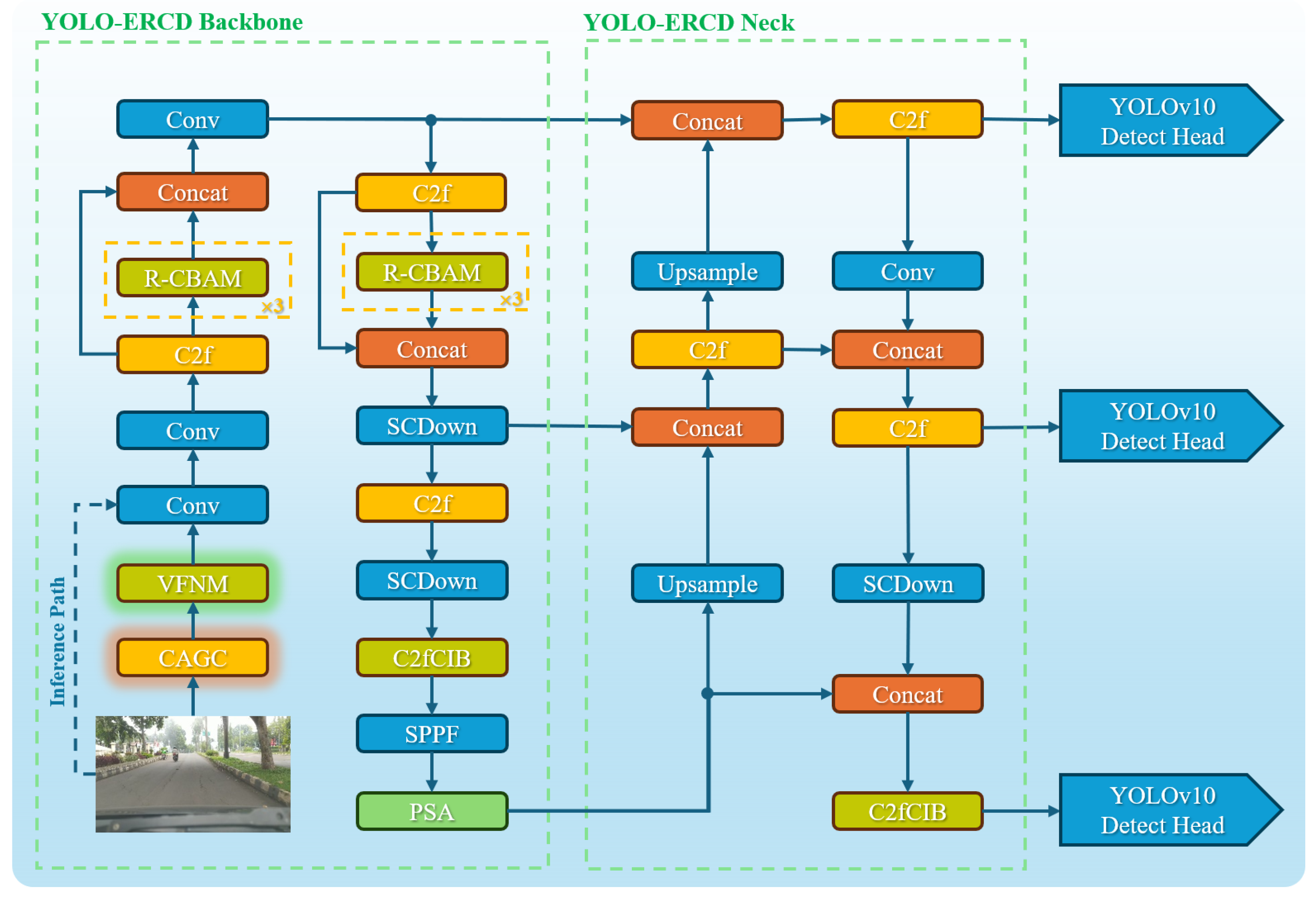
Overview of the YOLO-ERCD architecture. The model builds upon YOLOv10s, incorporating R-CBAM for enhanced spatial and channel attention, CAGC for adaptive illumination simulation, and VFNM for density-aware noise modulation. Standard components from YOLOv10s, such as C2fCIB, PSA, and SCDown, remain unchanged. The enhancements specifically target fine-grained road crack detection under challenging real-world conditions.
Figure 1.
Overview of the YOLO-ERCD architecture. The model builds upon YOLOv10s, incorporating R-CBAM for enhanced spatial and channel attention, CAGC for adaptive illumination simulation, and VFNM for density-aware noise modulation. Standard components from YOLOv10s, such as C2fCIB, PSA, and SCDown, remain unchanged. The enhancements specifically target fine-grained road crack detection under challenging real-world conditions.
Figure 2.
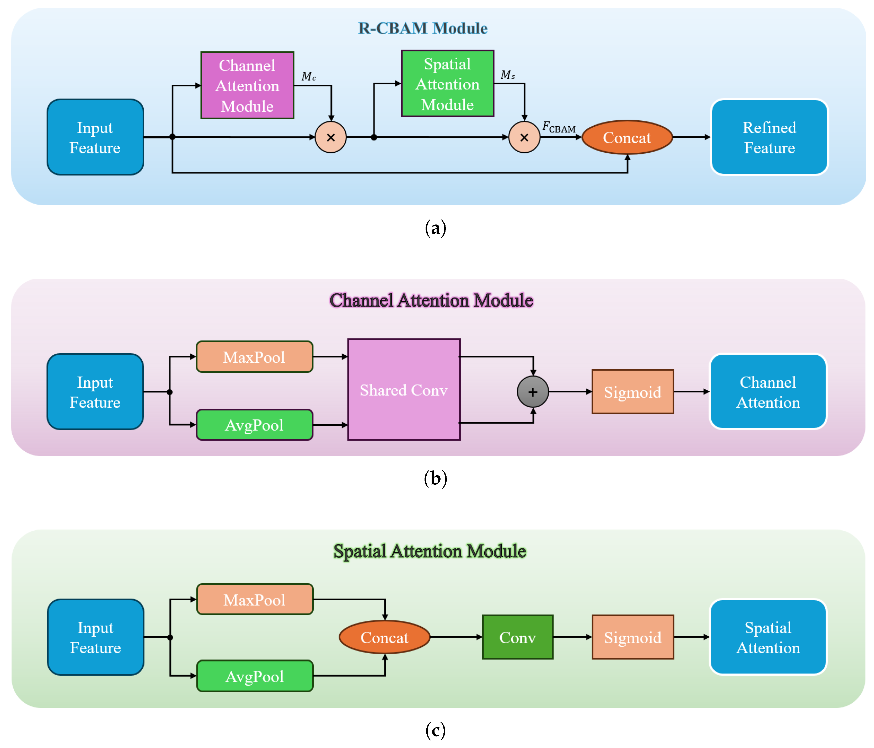
Detailed structure of the proposed Residual Convolutional Block Attention Module (R-CBAM). (a) Overall R-CBAM architecture, which concatenates the original feature map with the CBAM-refined features along the channel dimension to preserve essential information and enhance attention; (b) Channel Attention Module (CAM) for adaptive channel-wise weighting; (c) Spatial Attention Module (SAM) for emphasizing informative spatial locations.
Figure 2.
Detailed structure of the proposed Residual Convolutional Block Attention Module (R-CBAM). (a) Overall R-CBAM architecture, which concatenates the original feature map with the CBAM-refined features along the channel dimension to preserve essential information and enhance attention; (b) Channel Attention Module (CAM) for adaptive channel-wise weighting; (c) Spatial Attention Module (SAM) for emphasizing informative spatial locations.
Figure 3.
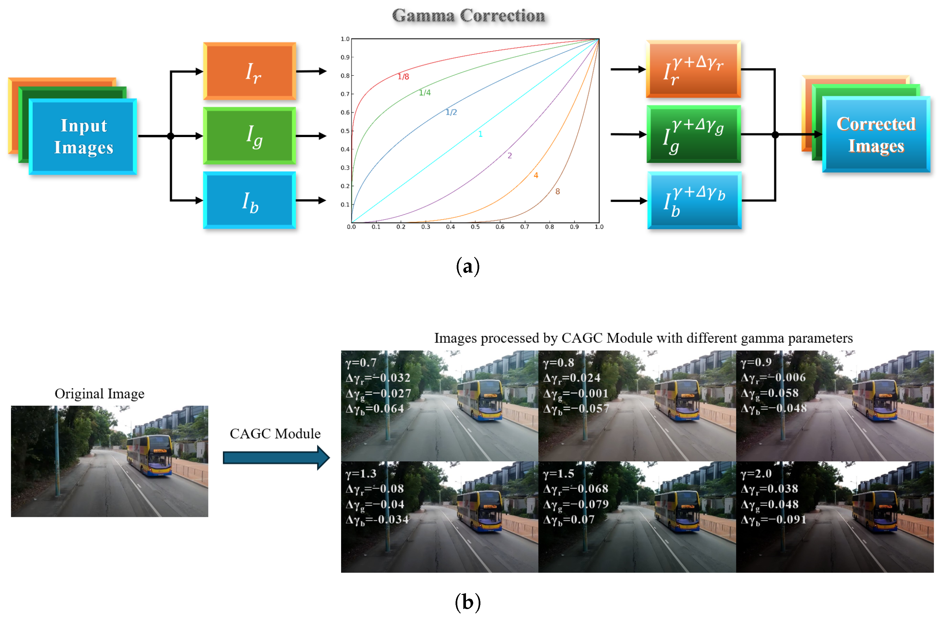
Visualization of the Channel-wise Adaptive Gamma Correction (CAGC) module. (a) Workflow of CAGC: input images are separated into RGB channels, and each channel undergoes gamma correction with a stochastically perturbed exponent to simulate diverse illumination conditions before being recombined as corrected images. (b) Example results: the left shows the original image, and the right demonstrates CAGC-processed images under different gamma settings, illustrating how channel-wise adaptive gamma perturbation enhances both bright and dark details for improved robustness to lighting variations.
Figure 3.
Visualization of the Channel-wise Adaptive Gamma Correction (CAGC) module. (a) Workflow of CAGC: input images are separated into RGB channels, and each channel undergoes gamma correction with a stochastically perturbed exponent to simulate diverse illumination conditions before being recombined as corrected images. (b) Example results: the left shows the original image, and the right demonstrates CAGC-processed images under different gamma settings, illustrating how channel-wise adaptive gamma perturbation enhances both bright and dark details for improved robustness to lighting variations.
Figure 4.
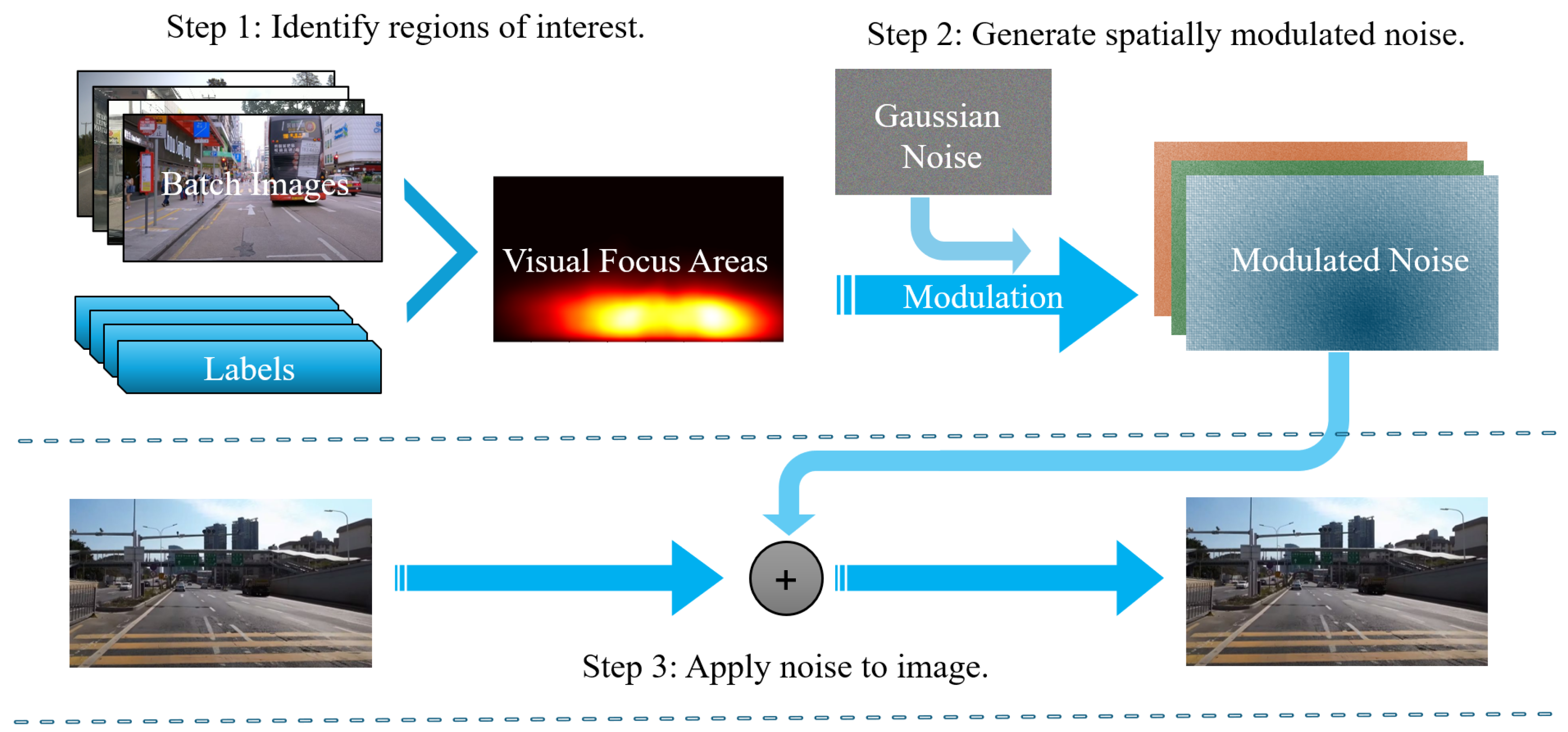
Workflow of the Visual Focus Noise Modulation (VFNM) module. Step 1: Regions of interest are identified from batch images and labels based on target density, generating a visual focus map. Step 2: Gaussian noise is spatially modulated according to the focus map, producing noise with reduced intensity in target-dense areas and stronger intensity in background regions. Step 3: The modulated noise is selectively applied to the input image, enhancing model robustness by protecting critical features while regularizing background areas.
Figure 4.
Workflow of the Visual Focus Noise Modulation (VFNM) module. Step 1: Regions of interest are identified from batch images and labels based on target density, generating a visual focus map. Step 2: Gaussian noise is spatially modulated according to the focus map, producing noise with reduced intensity in target-dense areas and stronger intensity in background regions. Step 3: The modulated noise is selectively applied to the input image, enhancing model robustness by protecting critical features while regularizing background areas.
Figure 5.
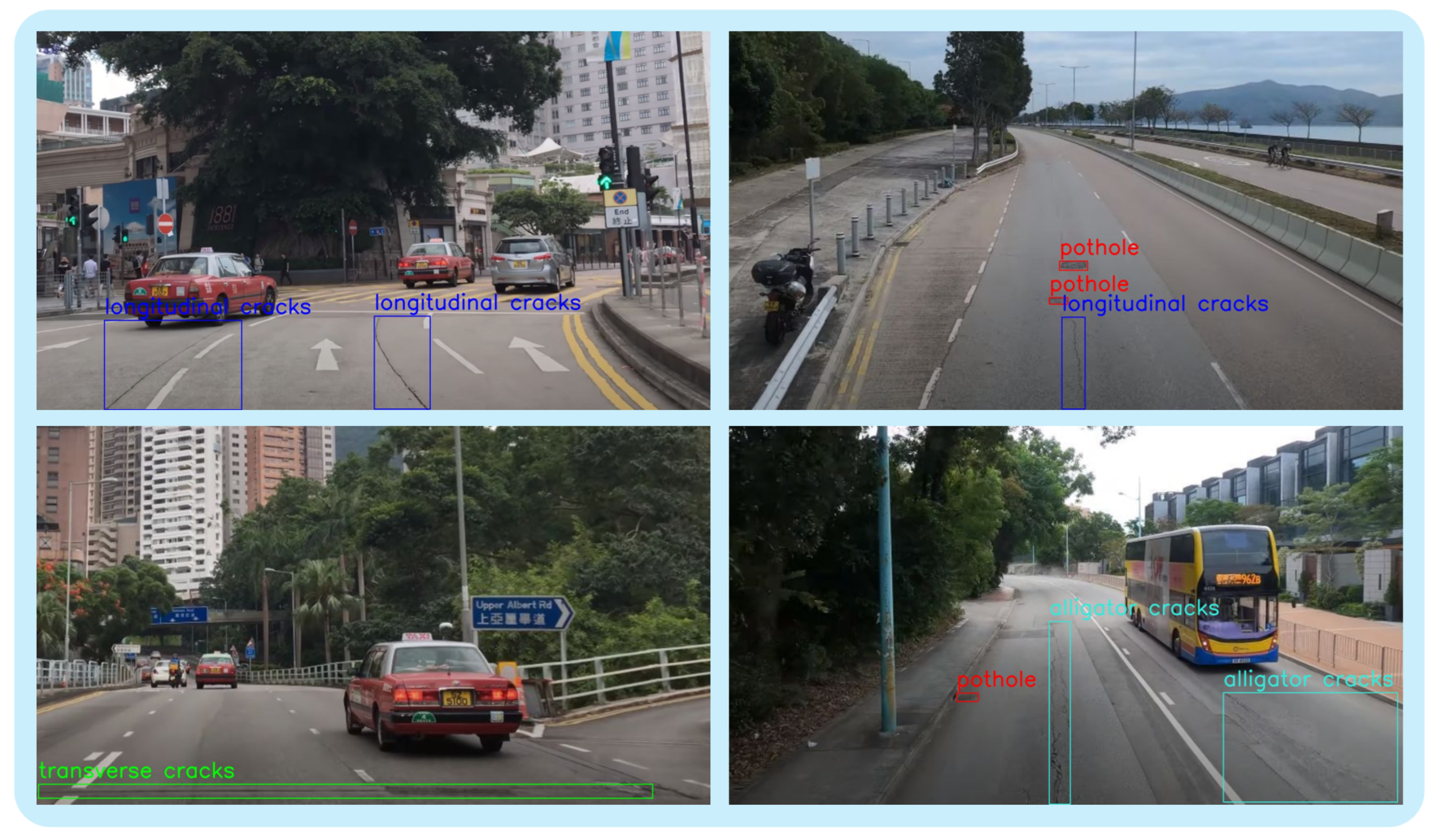
Sample images in the HKPC dataset.
Figure 5.
Sample images in the HKPC dataset.
Figure 6.
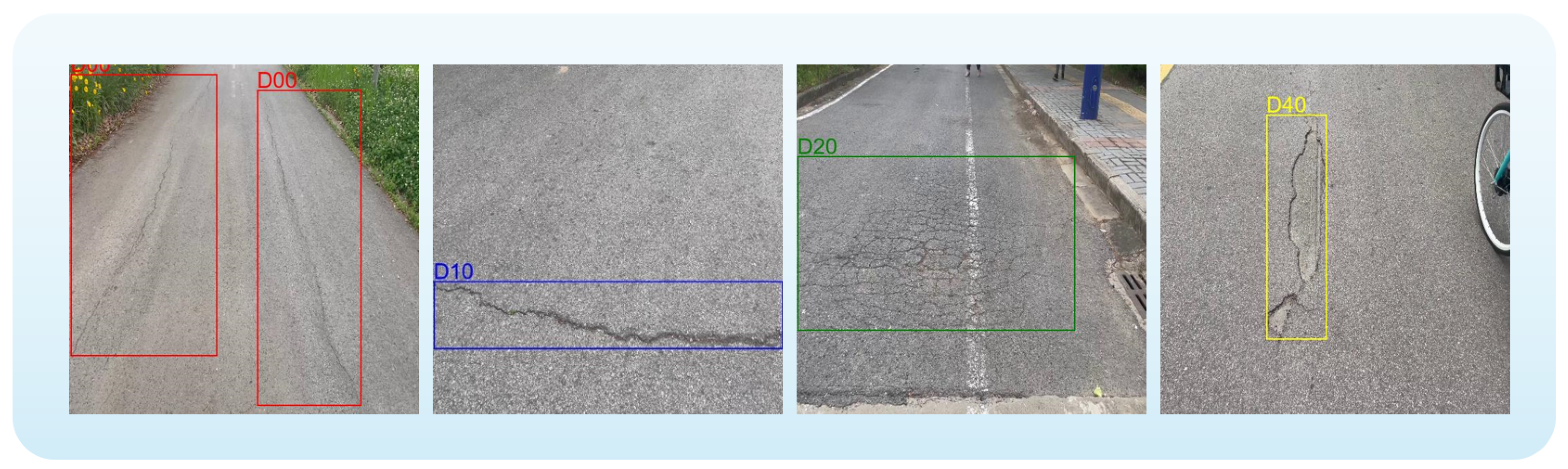
Sample images in the RDD2022 dataset, from left to right: longitudinal cracks (D00), transverse cracks (D10), alligator cracks (D20), and potholes (D40).
Figure 6.
Sample images in the RDD2022 dataset, from left to right: longitudinal cracks (D00), transverse cracks (D10), alligator cracks (D20), and potholes (D40).
Figure 7.
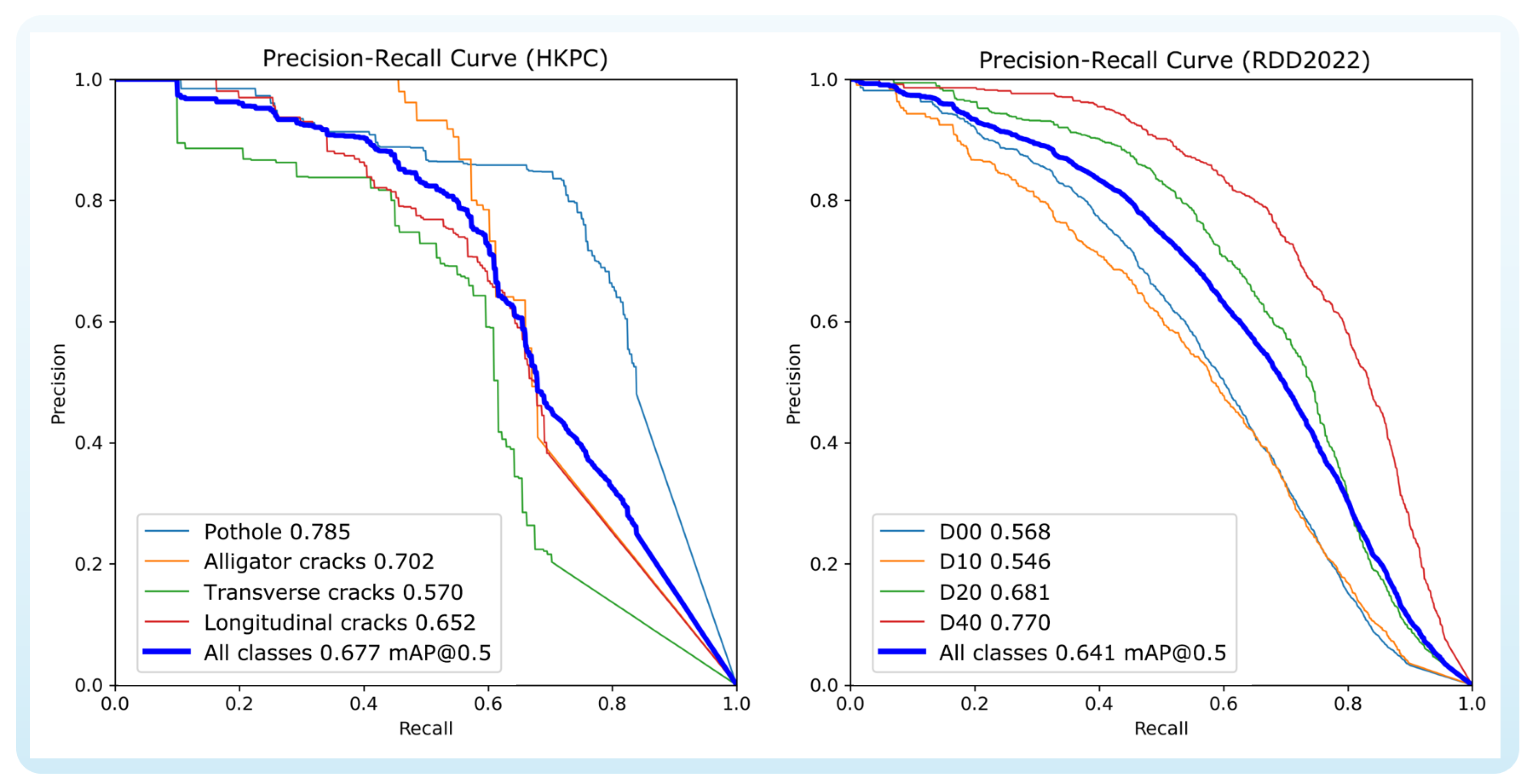
Precision–Recall curves by category (HKPC and RDD2022 dataset).
Figure 7.
Precision–Recall curves by category (HKPC and RDD2022 dataset).
Figure 8.
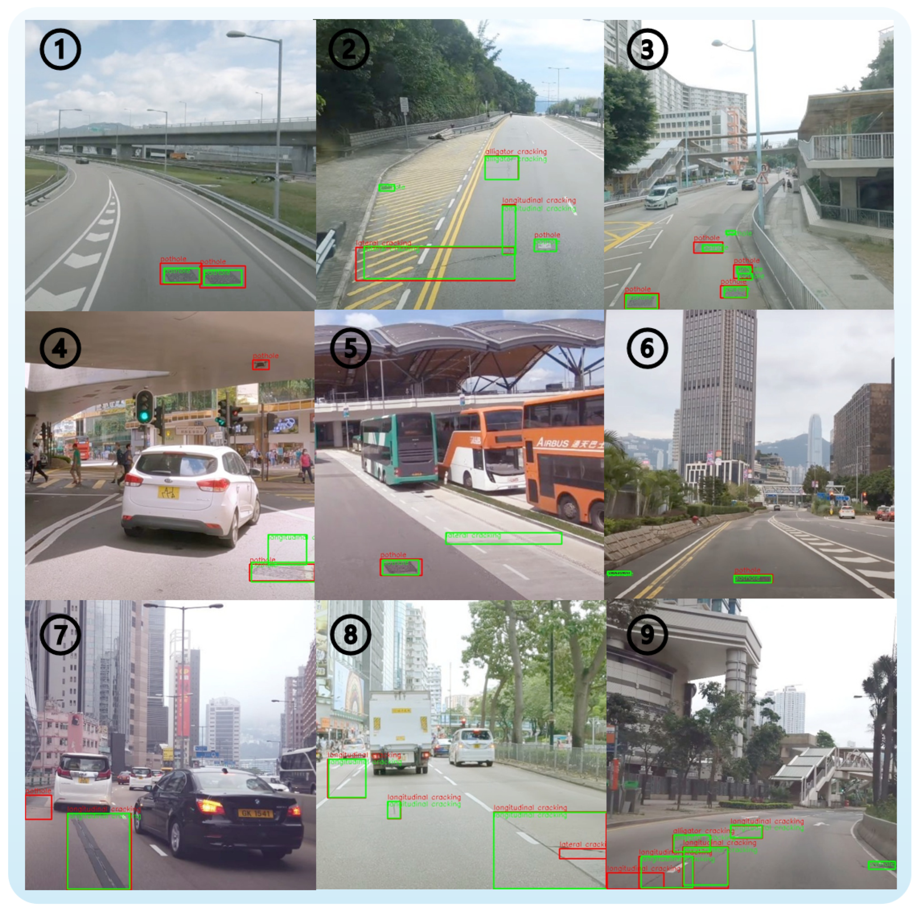
Qualitative analysis of typical false positive and false negative cases on the HKPC test set. Green boxes indicate ground truth, and red boxes represent model predictions. Each numbered example highlights a specific failure pattern related to blurred boundaries, complex morphology, low contrast, or texture interference.
Figure 8.
Qualitative analysis of typical false positive and false negative cases on the HKPC test set. Green boxes indicate ground truth, and red boxes represent model predictions. Each numbered example highlights a specific failure pattern related to blurred boundaries, complex morphology, low contrast, or texture interference.
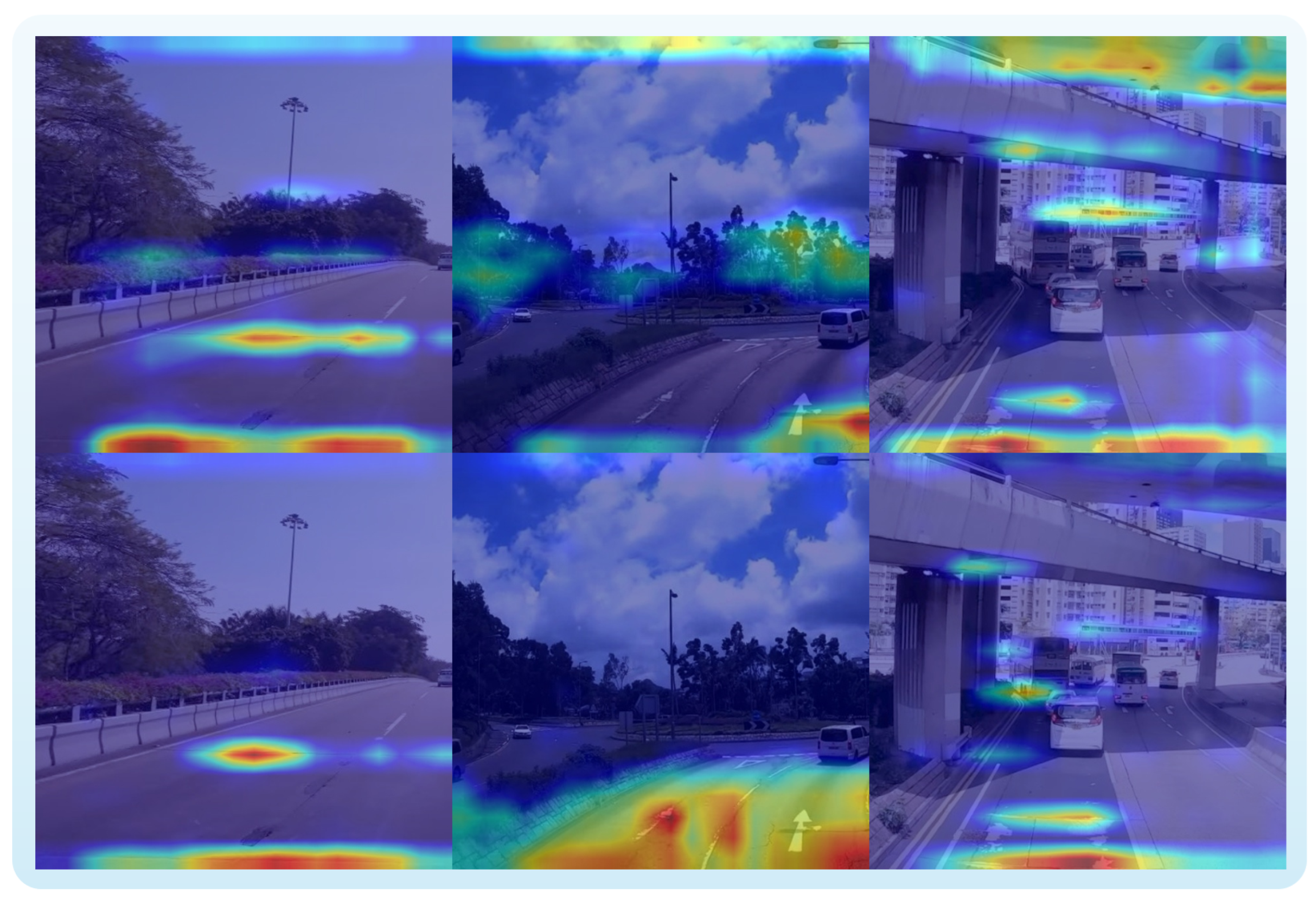
Figure 9.
Grad-CAM visualization of attention heatmaps for the same input image. Warmer colors (e.g., red) indicate regions with higher attention, while cooler colors (e.g., blue) indicate lower attention. The first row corresponds to the baseline YOLOv10s model, while the second row displays the improved YOLO-ERCD model with CAGC, R-CBAM, and VFNM modules. The YOLO-ERCD model demonstrates more focused and accurate attention on pavement damage regions, illustrating its enhanced interpretability and detection robustness.
Figure 9.
Grad-CAM visualization of attention heatmaps for the same input image. Warmer colors (e.g., red) indicate regions with higher attention, while cooler colors (e.g., blue) indicate lower attention. The first row corresponds to the baseline YOLOv10s model, while the second row displays the improved YOLO-ERCD model with CAGC, R-CBAM, and VFNM modules. The YOLO-ERCD model demonstrates more focused and accurate attention on pavement damage regions, illustrating its enhanced interpretability and detection robustness.
Table 1.
Comparison of Parameter and FLOPs Overhead Introduced by Stacking CBAM or R-CBAM Modules Three Times in the YOLOv10s Backbone. The table summarizes the model size and computational cost for the original YOLOv10s, YOLOv10s with CBAM stacked three times, and YOLOv10s with R-CBAM stacked three times.
Table 1.
Comparison of Parameter and FLOPs Overhead Introduced by Stacking CBAM or R-CBAM Modules Three Times in the YOLOv10s Backbone. The table summarizes the model size and computational cost for the original YOLOv10s, YOLOv10s with CBAM stacked three times, and YOLOv10s with R-CBAM stacked three times.
| Model | Parameters (M) | FLOPs (GFLOPs) | Parameter Increase (%) | FLOPs Increase (%) |
|---|
| YOLOv10s | 8.07 | 24.8 | – | – |
| YOLOv10s + CBAM (×3) | 8.12 | 24.8 | 0.6% | – |
| YOLOv10s + R-CBAM (×3) | 8.24 | 26.2 | 2.1% | 5.6% |
Table 2.
Distribution of sample numbers and proportions by road damage type in the HKPC dataset.
Table 2.
Distribution of sample numbers and proportions by road damage type in the HKPC dataset.
| Road Damage Type | Number of Samples | Proportion of Samples |
|---|
| Pothole | 7971 | 38.0% |
| Alligator cracks | 2892 | 13.8% |
| Transverse cracks | 3666 | 17.4% |
| Longitudinal cracks | 6468 | 30.8% |
| Total | 20,997 | 100% |
Table 3.
Distribution of sample numbers and proportions by road damage type in the RDD2022 dataset.
Table 3.
Distribution of sample numbers and proportions by road damage type in the RDD2022 dataset.
| Road Damage Type | Number of Samples | Proportion of Samples |
|---|
| Longitudinal cracks (D00) | 26,016 | 47.3% |
| Transverse cracks (D10) | 11,830 | 21.5% |
| Alligator cracks (D20) | 10,617 | 19.3% |
| Potholes (D40) | 6544 | 11.9% |
| Total | 55,007 | 100% |
Table 4.
Performance comparison of object detection models on the HKPC and RDD2022 datasets.
Table 4.
Performance comparison of object detection models on the HKPC and RDD2022 datasets.
| Model | mAP@0.5 (HKPC) | mAP@0.5 (RDD2022) | GFLOPs | Parameters (M) |
|---|
| Faster RCNN | 0.601 | 0.607 | 251.4 | 60.5 |
| RT-DETR-L | 0.623 | 0.619 | 108.3 | 32.8 |
| YOLOv5s | 0.572 | 0.567 | 24.0 | 9.1 |
| YOLOv8n | 0.621 | 0.618 | 8.7 | 3.0 |
| YOLOv8s | 0.625 | 0.623 | 28.4 | 11.1 |
| YOLOv8l | 0.633 | 0.628 | 164.8 | 43.6 |
| RDD-YOLO | 0.635 | 0.625 | 255.3 | 65.9 |
| YOLOv10s | 0.656 | 0.637 | 24.8 | 8.1 |
| YOLOv10l | 0.659 | 0.638 | 120.3 | 25.8 |
| YOLOv11s | 0.668 | 0.641 | 21.6 | 9.4 |
| YOLOv12s | 0.665 | 0.640 | 21.5 | 9.3 |
| YOLO-ERCD (Ours) | 0.677 | 0.641 | 26.2 | 8.2 |
Table 5.
Ablation study of YOLO-ERCD based on the YOLOv10s model.
Table 5.
Ablation study of YOLO-ERCD based on the YOLOv10s model.
| YOLOv10s | R-CBAM | CAGC | VFNM | mAP@0.5 |
|---|
| ✓ | | | | 0.656 |
| ✓ | ✓ | | | 0.665 |
| ✓ | | ✓ | | 0.662 |
| ✓ | | | ✓ | 0.665 |
| ✓ | | ✓ | ✓ | 0.667 |
| ✓ | ✓ | ✓ | | 0.668 |
| ✓ | ✓ | | ✓ | 0.675 |
| ✓ | ✓ | ✓ | ✓ | 0.677 |
Table 6.
Comparison of CBAM integration positions in YOLOv10s.
Table 6.
Comparison of CBAM integration positions in YOLOv10s.
| Position | mAP@0.5 |
|---|
| No CBAM | 0.656 |
| CBAM in Backbone | 0.661 |
| CBAM in Neck | 0.659 |
Table 7.
Comparison of CBAM and R-CBAM stacking in YOLOv10s (backbone).
Table 7.
Comparison of CBAM and R-CBAM stacking in YOLOv10s (backbone).
| Number of Stacked Layers | 1 | 2 | 3 | 4 |
|---|
| CBAM (mAP@0.5) | 0.661 | 0.653 | 0.622 | 0.6 |
| R-CBAM (mAP@0.5) | 0.662 | 0.664 | 0.665 | 0.665 |
Table 8.
Comparison of gamma correction strategies (mAP@0.5).
Table 8.
Comparison of gamma correction strategies (mAP@0.5).
| Gamma Correction Strategy | mAP@0.5 |
|---|
| No gamma correction | 0.656 |
| Random gamma correction | 0.658 |
| CAGC Module (Proposed) | 0.662 |
Table 9.
Comparison of VFNM and Gaussian noise augmentation (different noise levels).
Table 9.
Comparison of VFNM and Gaussian noise augmentation (different noise levels).
| Noise Level () | 5 | 10 | 15 | 20 | 25 |
|---|
| Gaussian Noise Augmentation | 0.659 | 0.658 | 0.586 | N/A 1 | N/A 1 |
| VFNM Module | 0.661 | 0.665 | 0.651 | 0.643 | 0.622 |
Table 10.
Performance of the model across categories in the HKPC test set.
Table 10.
Performance of the model across categories in the HKPC test set.
| Class | Precision | Recall | AP@0.5 | AP@0.5:0.95 |
|---|
| Pothole | 0.798 | 0.737 | 0.785 | 0.422 |
| Alligator cracks | 0.867 | 0.573 | 0.702 | 0.405 |
| Transverse cracks | 0.662 | 0.570 | 0.570 | 0.245 |
| Longitudinal cracks | 0.688 | 0.594 | 0.652 | 0.349 |
| All (mean) | 0.754 | 0.618 | 0.677 | 0.355 |
Table 11.
Performance of the model across categories in the RDD2022 test set.
Table 11.
Performance of the model across categories in the RDD2022 test set.
| Class | Precision | Recall | AP@0.5 | AP@0.5:0.95 |
|---|
| Longitudinal cracks (D00) | 0.634 | 0.507 | 0.568 | 0.329 |
| Transverse cracks (D10) | 0.623 | 0.482 | 0.546 | 0.284 |
| Alligator cracks (D20) | 0.682 | 0.627 | 0.681 | 0.370 |
| Pothole (D40) | 0.679 | 0.731 | 0.770 | 0.488 |
| All (mean) | 0.655 | 0.587 | 0.641 | 0.368 |