
Single-Phase Grounding Fault Types Identification Based on Multi-Feature Transformation and Fusion

Abstract
:1. Introduction
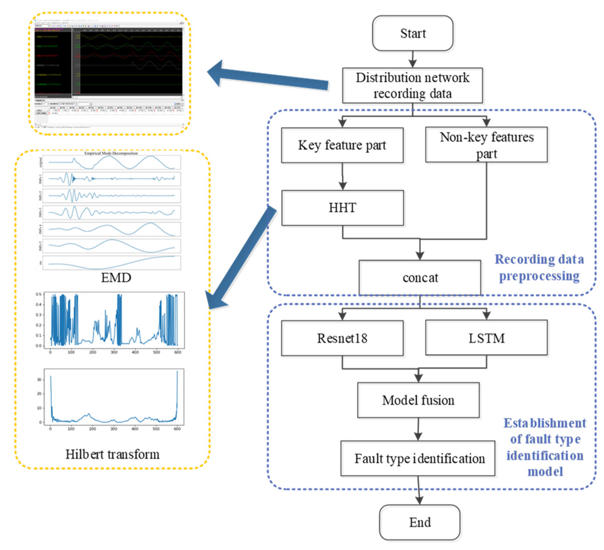
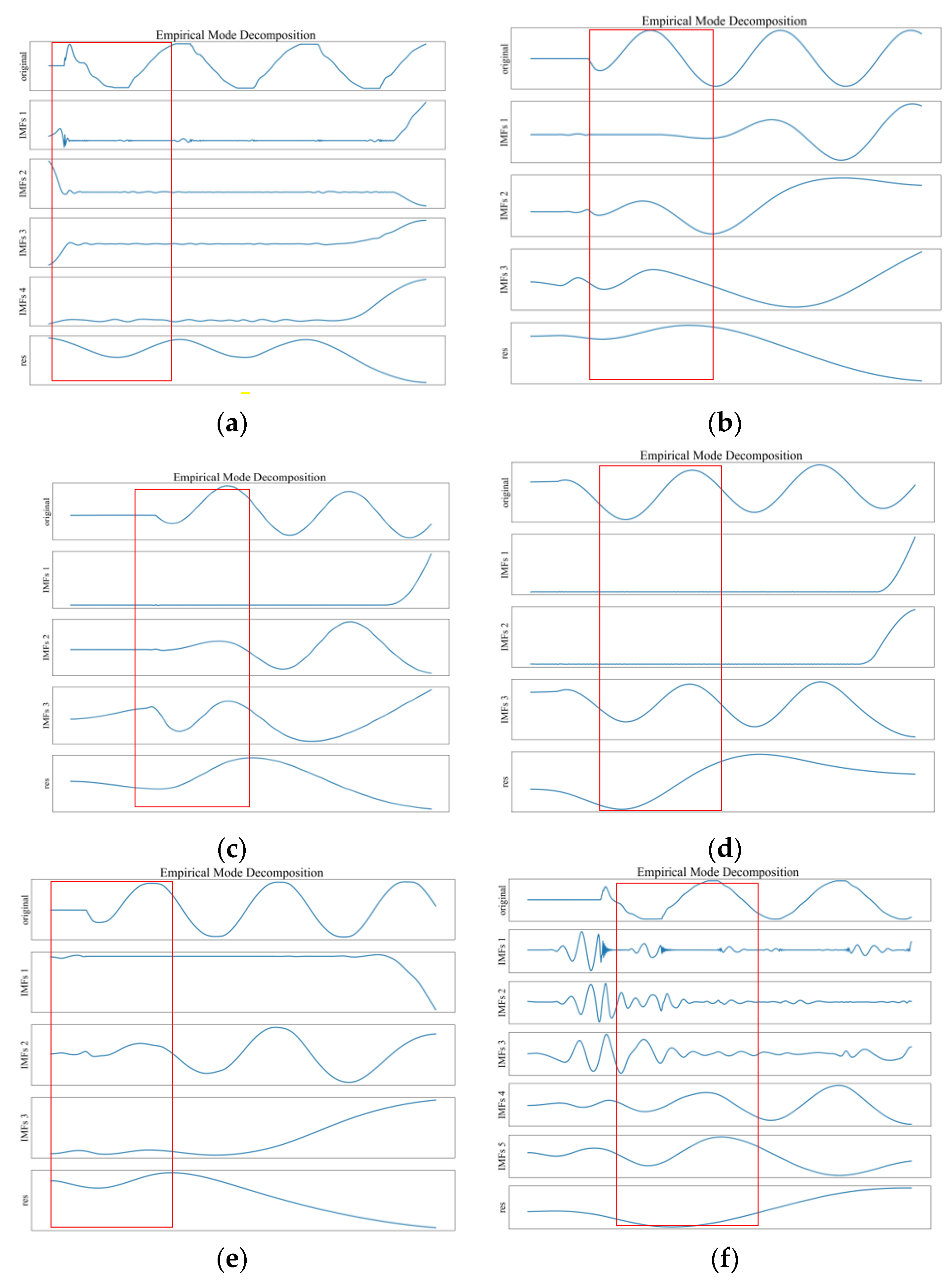
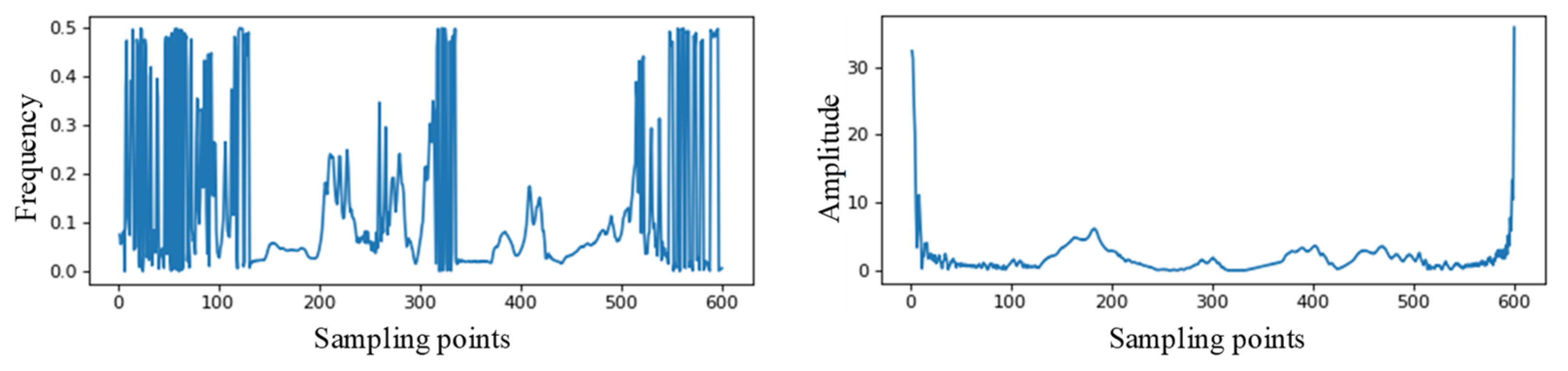
- A time–frequency analysis method, Hilbert–Huang transform with strong adaptive capability, was used in the data preprocessing part and was helpful for extracting the transient characteristics of faults and highlighting the characteristics of different fault types.
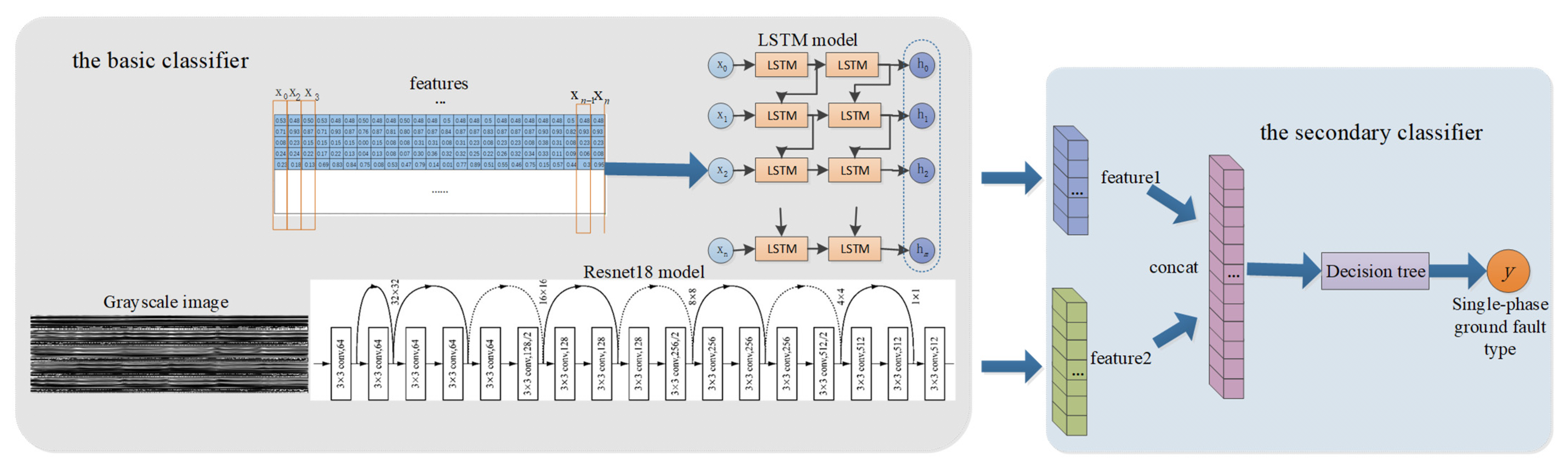
- The deep learning models ResNet18 and LSTM were designed to extract the complex abstract features related to the fault type from preprocessed data set, including complex nonlinear features and timing correlation features.
- A single-phase ground fault type identification model was constructed based on the idea of model fusion, which combines the advantages of heterogeneous models to enhance the overall identification accuracy and robustness of the model.
2. Related Works
2.1. Comparison of Related Works
2.2. Principles of the Related Knowledge
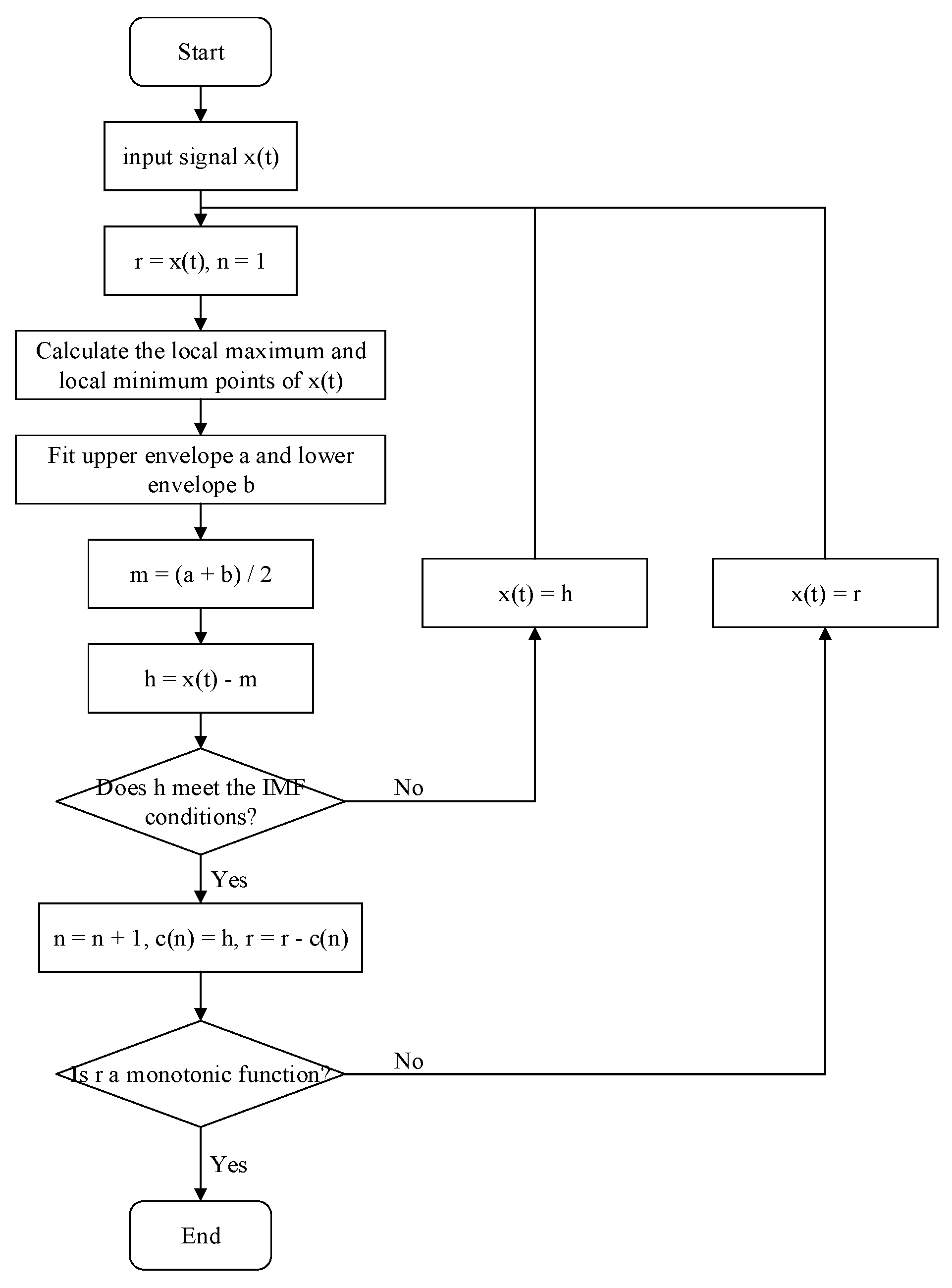
2.2.1. Principle of Hilbert–Huang Transform
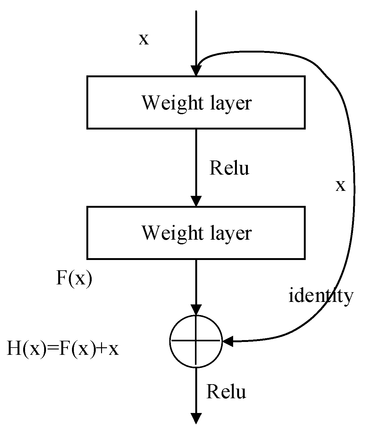
2.2.2. Principle of Resnet18 Network
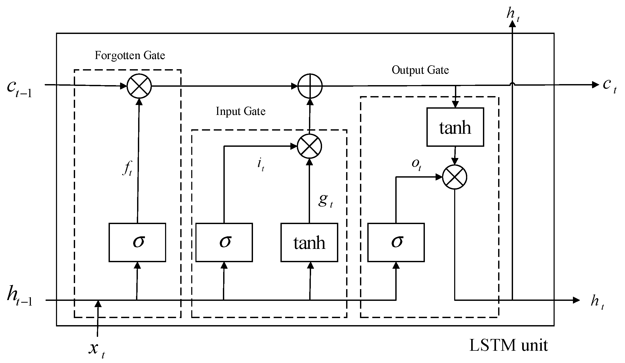
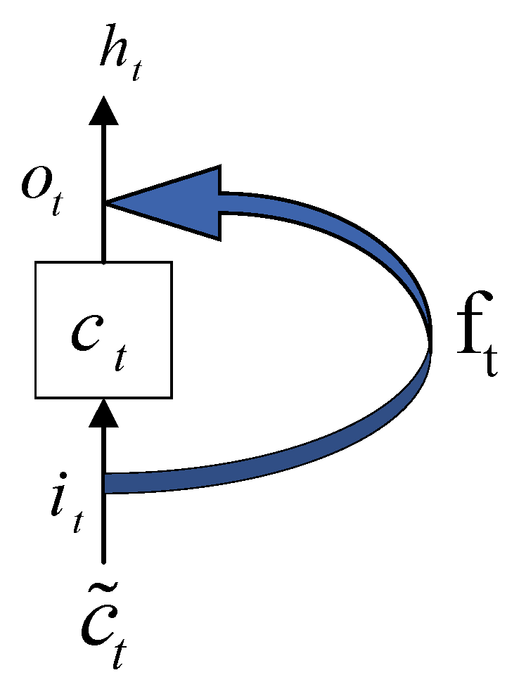
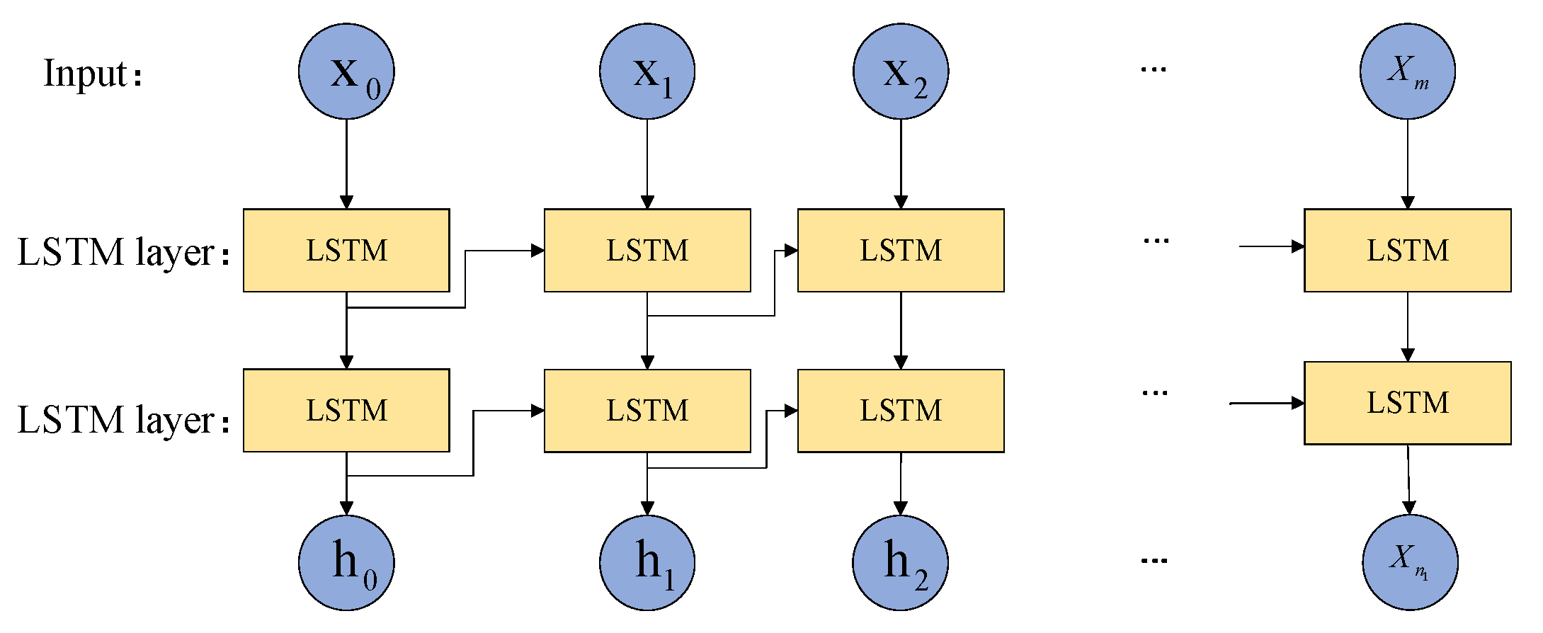
2.2.3. Principle of Long Short-Term Memory (LSTM) Network
3. Problem Formulation and Methodology
3.1. Data Preprocessing
3.2. Single-Phase Ground Fault-Type Identification Model
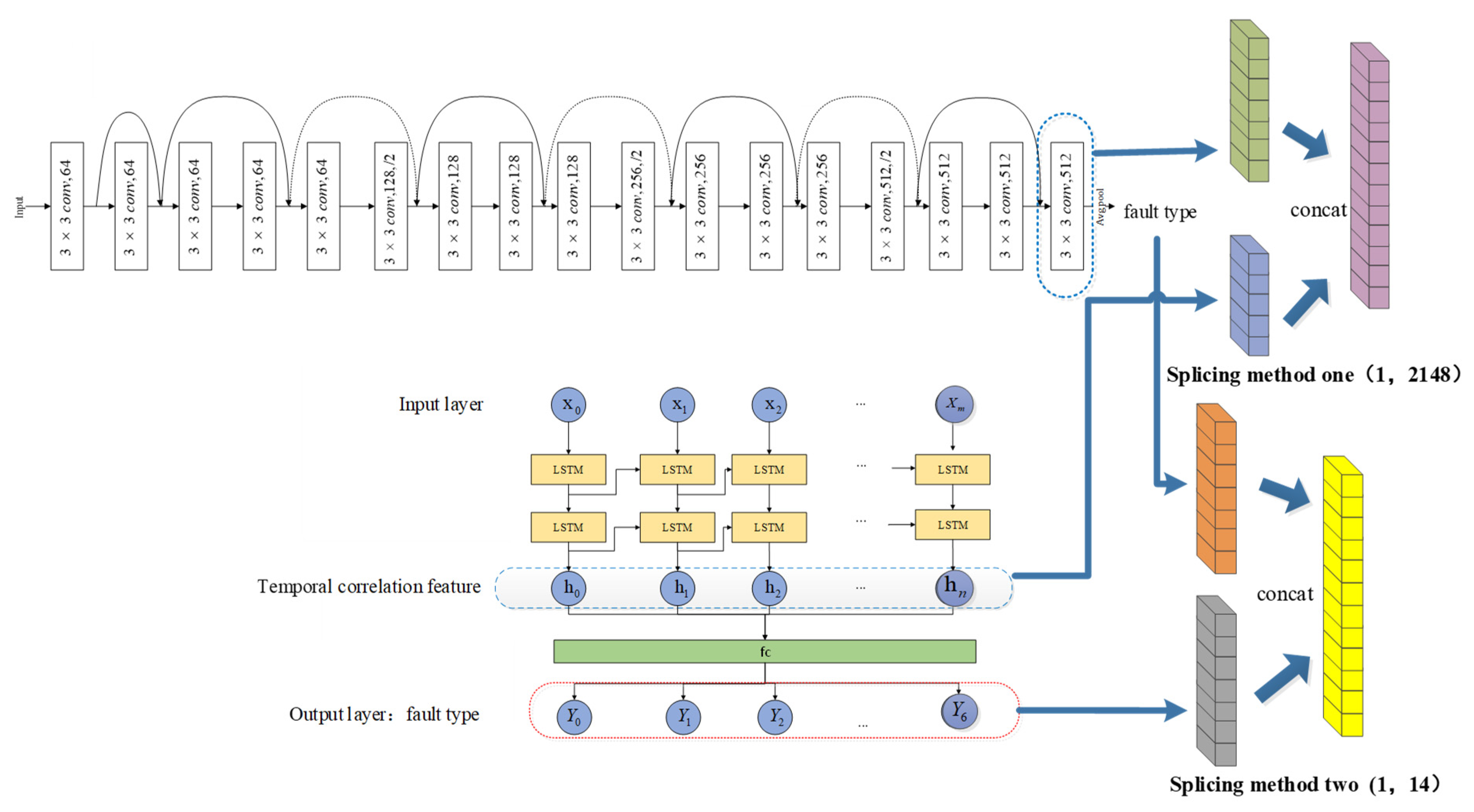
3.2.1. The Overall Structure of the Model
3.2.2. Extracting Complex Nonlinear Features Based on the Adjusted Resnet18 Model
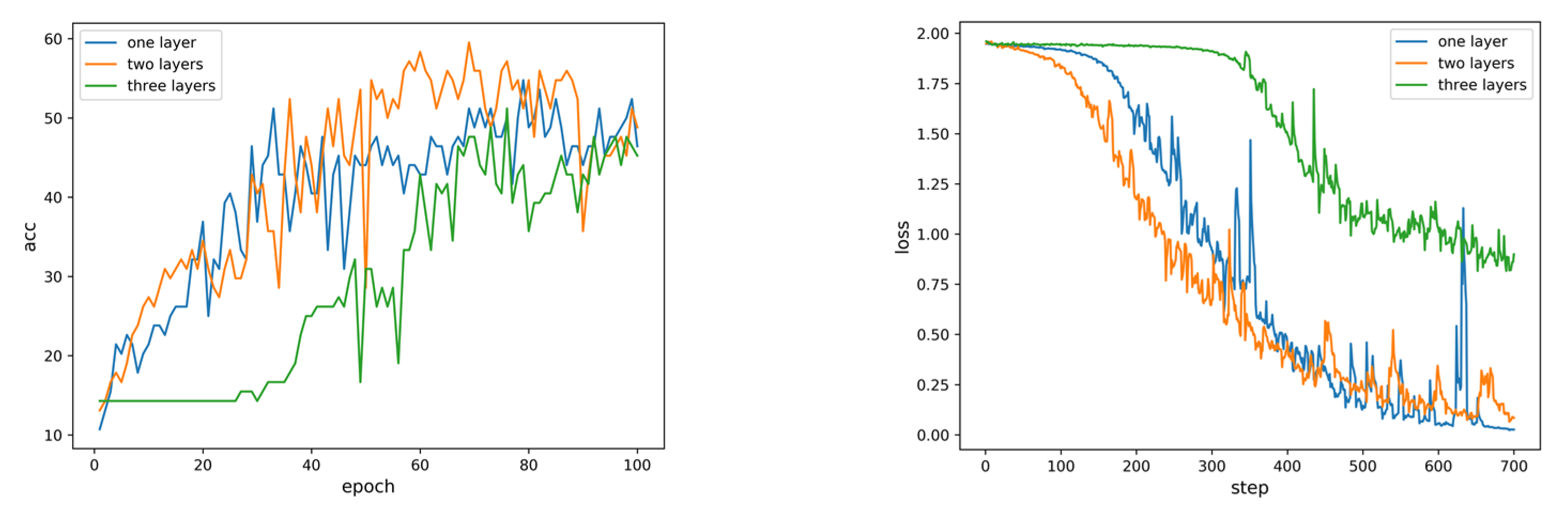
3.2.3. Extracting Timing Correlation Features Based on the Adjusted LSTM Model
3.2.4. Construction of the Secondary Data Sets and Fusion Models
4. Analysis of Results
4.1. Establishment of Training Set and Testing Set
4.2. Evaluation Index
4.3. Design and Analysis of Experiments
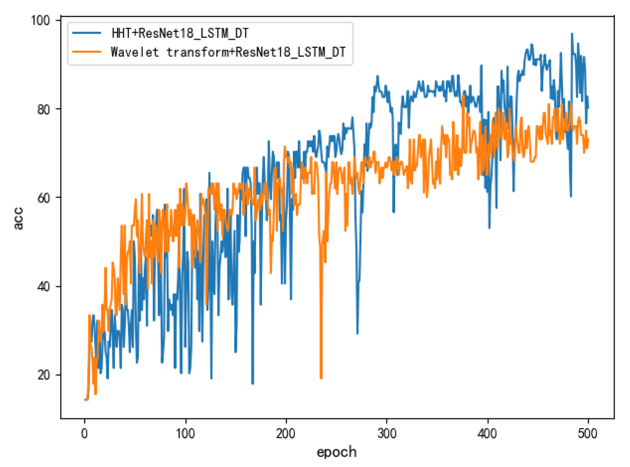
4.3.1. Performance Comparison of Time–Frequency Analysis Methods
4.3.2. Performance Analysis of the Preprocessing Methods
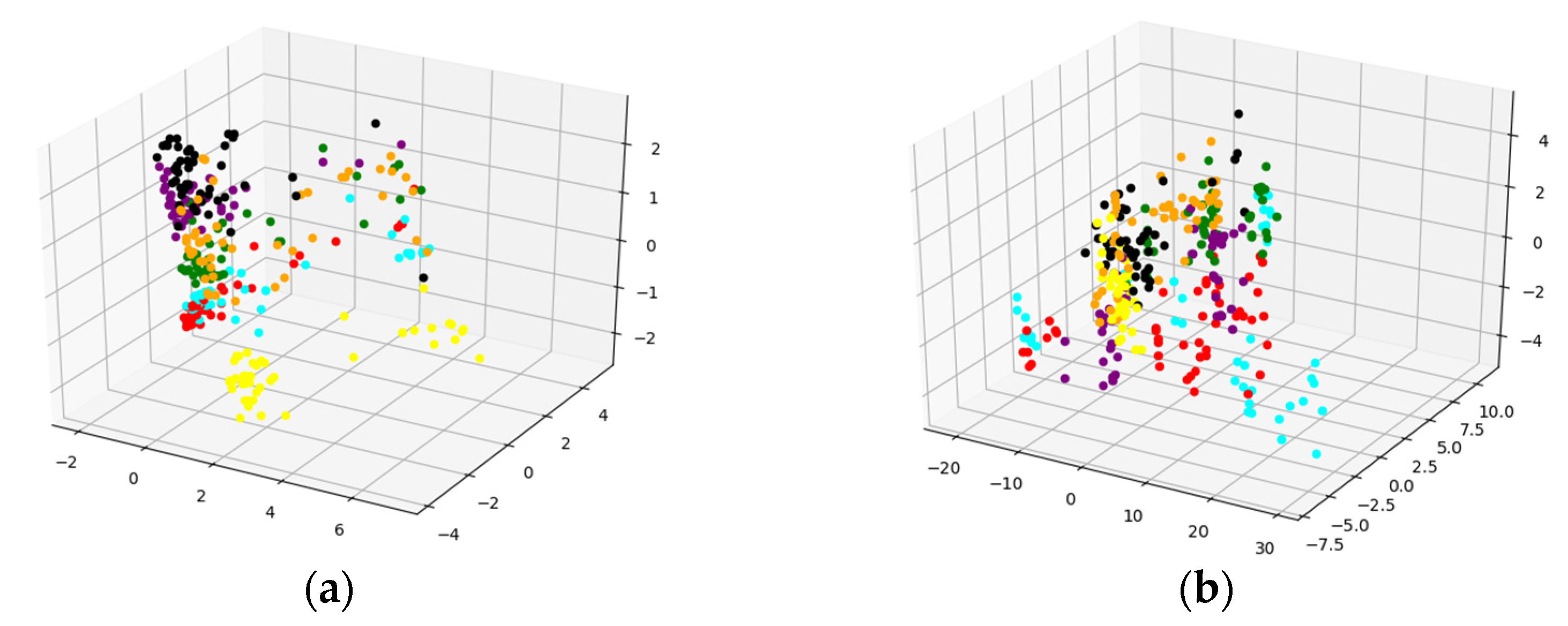
4.3.3. Performance Analysis of Fusion Process
4.3.4. Performance Analysis of the Fusion Model and Single Model
4.3.5. Comparison with AlexNet
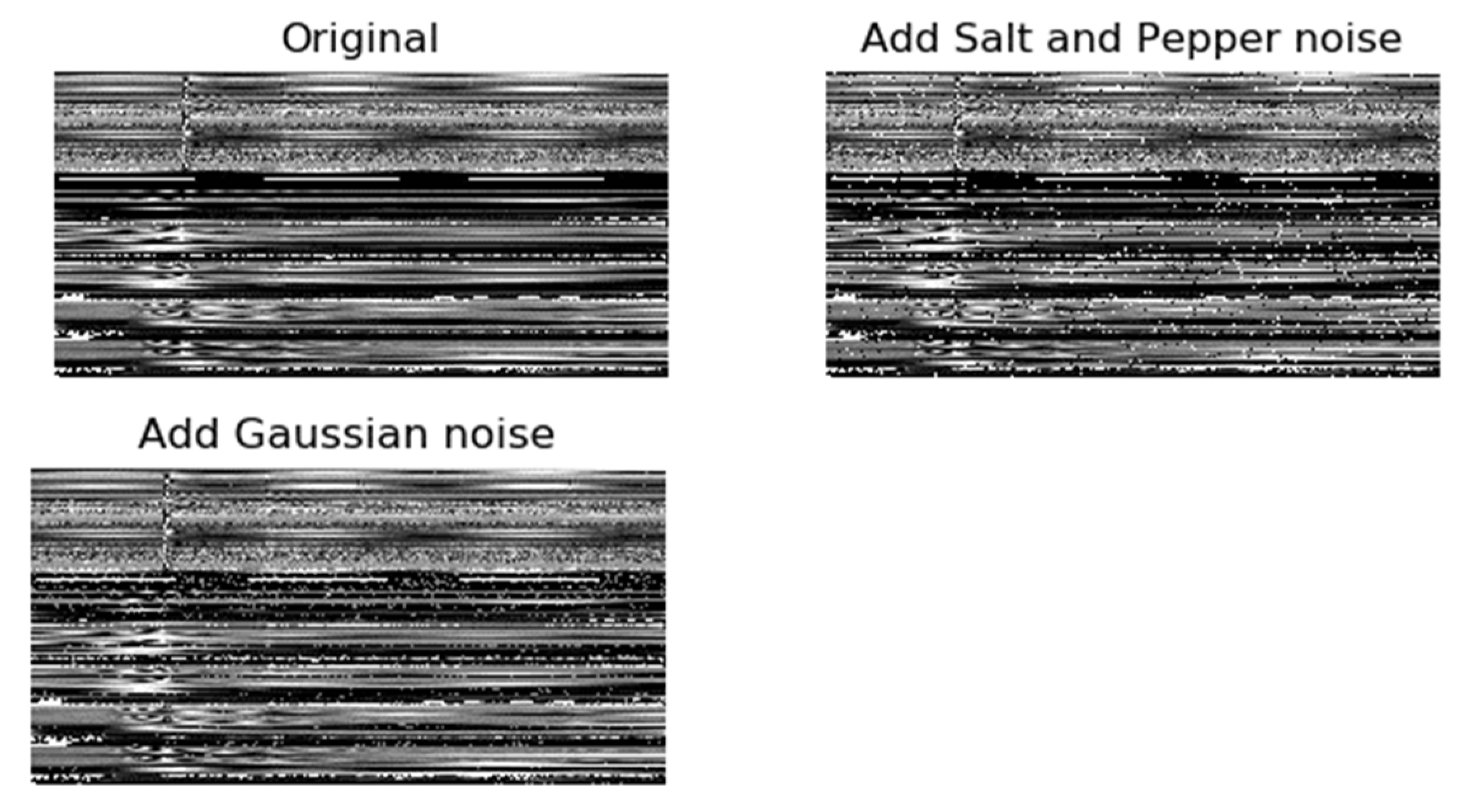
4.3.6. Robust Performance
5. Conclusions and Future Work
- The method proposed in this paper is only based on the fault recorded wave data collected by the wave recorder for analysis. With the improvement of information collection devices and transmission systems in power systems, more characteristic data related to single-phase ground fault types can be obtained, such as: ledger data, attribute data, external data including environmental data and weather data, etc. It can also be included on the basis of fault type identification for analysis.
- The single-phase grounding fault has the problem of imbalance between the fault data and the normal data, and the imbalance between the various fault types, which will affect the classification accuracy of the identification model. Follow-up research may analyze and consider this.
Author Contributions
Funding
Institutional Review Board Statement
Informed Consent Statement
Data Availability Statement
Conflicts of Interest
References
- Zhang, Z. Theoretical Research on Single-Phase Grounding Fault Line Selection in Small Current Grounding System; Liaoning Science and Technology Press: Dalian, China, 2014; pp. 6–12. [Google Scholar]
- Elmitwally, A.; Ghanem, A. Local current-based method for fault identification and location on series capacitor-compensated transmission line with different configurations. Int. J. Electr. Power Energy Syst. 2021, 133, 107283. [Google Scholar] [CrossRef]
- Li, J.; Wang, G.; Zeng, D.; Li, H. High-impedance ground faulted line-section location method for a resonant grounding system based on the zero-sequence current’s declining periodic component. Int. J. Electr. Power Energy Syst. 2020, 19, 105910. [Google Scholar] [CrossRef]
- Liu, K.; Zhang, S.; Li, B.; Zhang, C.; Liu, B.; Jin, H.; Zhao, J. Faulty Feeder Identification Based on Data Analysis and Similarity Comparison for Flexible Grounding System in Electric Distribution Networks. Sensors 2021, 21, 154. [Google Scholar] [CrossRef] [PubMed]
- Zhou, F.; Zhu, R.; Wang, C.; Wang, B.; Liu, J. Online criterion and identification of single-phase ground fault with high resistence in distribution network. Chin. J. Sci. Instrum. 2015, 36, 685–693. [Google Scholar]
- Shen, Y.; Ruan, L.; Dai, B.; Liu, N.; Qiu, L.; He, X. Identification of single-phase arc grounding fault in power distribution network. J. Wuhan Univ. 2018, 51, 1098–1104. [Google Scholar]
- Wang, B.; Geng, J.; Dong, X. High-Impedance Fault Detection Based on Nonlinear Voltage-Current Characteristic Profile Identification. IEEE Trans. Smart Grid 2016, 9, 3783–3791. [Google Scholar] [CrossRef]
- Chen, M.; Hang, Y.; Zhai, J. High impedance fault identification method of distribution network. J. Chongqing Univ. 2013, 36, 83–88. [Google Scholar]
- Ji, P.; Pei, Y.; Zhao, S.; Bai, C.; Wu, B.; Liang, L.; Pin, D.; Sun, H.; Zhi, T. A Novel Location Method for Single-phase Grounding Fault for Distribution Network Based on Transient Technique. In Proceedings of the 2018 Chinese Control And Decision Conference (CCDC), Shenyang, China, 9–11 June 2018; pp. 5190–5193. [Google Scholar]
- Zhou, J.; Ayhan, B.; Kwan, C.; Liang, S.; Lee, W. High-Performance Arcing-Fault Location in Distribution Networks. IEEE Trans. Ind. Appl. 2012, 48, 1107–1114. [Google Scholar] [CrossRef]
- Chen, Z.; Li, Y.; Peng, H.; Liu, W. Identification of Single-phase High Resistance Earth Fault in Distribution Network Based on Wavelet Packet Energy Ratio of Zero Sequence Voltage. Sci. Technol. Eng. 2020, 20, 8202–8209. [Google Scholar]
- Shao, W.; Bai, J.; Cheng, Y.; Zhang, Z.; Li, N. Research on a Faulty Line Selection Method Based on the Zero-Sequence Disturbance Power of Resonant Grounded Distribution Networks. Energies 2019, 12, 846. [Google Scholar] [CrossRef] [Green Version]
- Guo, M.; Liu, S.; Yang, G. Grounding Faulty line detection based on transient waveform difference recognition for resonant earthed system. Electr. Power Autom. Equip. 2014, 34, 59–66. [Google Scholar]
- Sheng, Y.; Cong, W.; Bu, X.; Li, X. Detection method of high impedance grounding fault based on differential current of zero-sequence current projection and neutral point current in low-resistance grounding system. Electr. Power Autom. Equip. 2019, 39, 7. [Google Scholar]
- Li, Z.; Ye, Y.; Ma, X.; Lin, X.; Ding, C. Single-phase-to-ground fault section location in flexible resonant grounding distribution networks using soft open points. Int. J. Electr. Power Energy Syst. 2020, 122, 106198. [Google Scholar] [CrossRef]
- Nakho, A.; Hamam, Y. Detection and Classification of Single Phase to Ground Faults Under High Resistance Ground Paths in Power Systems using Machine Learning. In Proceedings of the 2021 Southern African Universities Power Engineering Conference/Robotics and Mechatronics/Pattern Recognition Association of South Africa (SAUPEC/RobMech/PRASA), Potchefstroom, South Africa, 27–29 January 2021. [Google Scholar]
- Sun, W.; Paiva, A.; Xu, P.; Sundaram, A.; Braatz, R.D. Fault detection and identification using Bayesian recurrent neural networks. Comput. Chem. Eng. 2020, 141, 106991. [Google Scholar] [CrossRef]
- Zhu, J.; Chen, K.; Peng, Z.; Zhang, H.; Wan, X.; Zhu, D. Single-phase ground fault identification method for distribution network based on inception model and sample expansion. J. Phys. Conf. Ser. 2020, 1656, 012008. [Google Scholar] [CrossRef]
- Tong, Y.; You, Z.; Shu, L. Analysis of Intermittent Arc Overvoltages in Low Resistance Grounded Systems; The Chinese Society of Universities for Electric Power System and Its Automation: Xiamen, China, 2012. [Google Scholar]
- Zhang, J.; Li, Y.; Zhang, Z.; Zeng, Z.; Cao, Y. XGBoost Classifier for Fault Identification in Low Voltage Neutral Point Ungrounded System. In Proceedings of the 2019 IEEE Sustainable Power and Energy Conference (iSPEC), Beijing, China, 21–23 November 2019. [Google Scholar]
- Dong, X.; Shi, S. Identifying Single-Phase-to-Ground Fault Feeder in Neutral Noneffectively Grounded Distribution System Using Wavelet Transform. Electr. Power Sci. Eng. 2011, 23, 1829–1837. [Google Scholar]
- Ni, G.; Bao, H.; Zhang, L.; Yang, Y. Criterion Based on the Fault Component of Zero Sequence Current for Online Fault Location of Single-phase Fault in Distribution Network. Proc. CSEE 2010, 30, 118–122. [Google Scholar]
- Liang, J. Research on Rapid Diagnosis Method of Single-Phase Grounding Fault in Distribution Network Based on Deep Learning. In Proceedings of the 2019 Chinese Automation Congress (CAC), Hangzhou, China, 22–24 November 2019; pp. 20–24. [Google Scholar]
- Srikanth, P.; Koley, C. A novel three-dimensional deep learning algorithm for classification of power system faults. Comput. Electr. Eng. 2021, 91, 107100. [Google Scholar] [CrossRef]
- Zhang, L.; Wang, Y.; Yan, H.; Shi, F. Single-phase-to-ground Fault Diagnosis Based on Waveform Feature Extraction and Matrix Analysis. In Proceedings of the 2019 9th International Conference on Power and Energy Systems (ICPES), Perth, Australia, 10–12 December 2019; pp. 1–6. [Google Scholar]
- Zhong, B.; Li, Y. Image Feature Point Matching Based on Improved SIFT Algorithm. In Proceedings of the 2019 IEEE 4th International Conference on Image, Vision and Computing (ICIVC), Xiamen, China, 5–7 July 2019; pp. 489–493. [Google Scholar]
- Zhang, P.; Shen, L.; Huang, X.; Xin, Q. Application of an Improved SIFT algorithm in GPR images. In Proceedings of the 2020 5th International Conference on Mechanical, Control and Computer Engineering (ICMCCE), Harbin, China, 25–27 December 2020; pp. 2201–2205. [Google Scholar]
- Zhao, M.; Qiu, W.; Wen, T.; Liao, T.; Huang, J. Feature extraction based on Gabor filter and Support Vector Machine classifier in defect analysis of Thermoelectric Cooler Component. Comput. Electr. Eng. 2021, 92, 107188. [Google Scholar] [CrossRef]
- Zhang, T.; Zhang, X.; Ke, X.; Liu, C.; Xu, X.; Zhan, X.; Wang, C.; Ahmad, I. HOG-ShipCLSNet: A Novel Deep Learning Network With HOG Feature Fusion for SAR Ship Classification. IEEE Trans. Geosci. Remote Sens. 2022, 60, 1–22. [Google Scholar] [CrossRef]
- Muhathir; Rizal, R.A.; Sihotang, J.S.; Gultom, R. Comparison of SURF and HOG extraction in classifying the blood image of malaria parasites using SVM. In Proceedings of the 2019 International Conference of Computer Science and Information Technology (ICoSNIKOM), Medan, Indonesia, 28–29 November 2019; pp. 1–6. [Google Scholar]
- Liu, Z.; Peng, D.; Zuo, M.J.; Xia, J.; Qin, Y. Improved Hilbert–Huang transform with soft sifting stopping criterion and its application to fault diagnosis of wheelset bearings. ISA Trans. 2021. [Google Scholar] [CrossRef] [PubMed]
- Shaik, M.; Shaik, A.G.; Yadav, S.K. Hilbert-Huang transform and decision tree based islanding and fault recognition in renewable energy penetrated distribution system. Sustain. Energy Grids Netw. 2022, 30, 100606. [Google Scholar] [CrossRef]
- Mahata, S.; Shakya, P.; Babu, N.R. A robust condition monitoring methodology for grinding wheel wear identification using Hilbert Huang transform. Precis. Eng. 2021, 3, 77–91. [Google Scholar] [CrossRef]
- Wang, Y.; Xu, H.; Yi, J.; Liang, S. Distribution Feeder Ground Fault Location Based on Hilbert-Huang Transform. J. Electr. Eng. 2020, 15, 18–26. [Google Scholar]
- Tan, Y.; Li, Y.; Liu, H.; Lu, W.; Xiao, X. Performance Comparison of Data Classification based on Modern Convolutional Neural Network Architectures. In Proceedings of the 2020 39th Chinese Control Conference (CCC), Shenyang, China, 27–29 July 2020. [Google Scholar]
- Zhang, R.; El-Gohary, N. A deep neural network-based method for deep information extraction using transfer learning strategies to support automated compliance checking. Autom. Constr. 2021, 132, 103834. [Google Scholar] [CrossRef]
- Yu, X.; Wang, S. Abnormality Diagnosis in Mammograms by Transfer Learning Based on ResNet18. Fundam. Inform. 2019, 168, 219–230. [Google Scholar] [CrossRef]
- Zagoruyko, S.; Komodakis, N. Wide Residual Networks. In Proceedings of the 2016 British Machine Vision Conference, York, UK, 19–22 September 2016; Volume 87, pp. 1–12. [Google Scholar]
- Lindemann, B.; Maschler, B.; Sahlab, N.; Weyrich, M. A survey on anomaly detection for technical systems using LSTM networks. Comput. Ind. 2021, 131, 103498. [Google Scholar] [CrossRef]
- Shao, Q.; Guo, L.; Liu, Y.; Xie, M.; Dai, C.; Wang, T.; Zhang, J.; Cong, Z. Identification Method for Single-phase Ground Fault of Distribution Network Based on LSTM Model. Guangdong Electr. Power 2019, 32, 100–106. [Google Scholar]
- Yue, Y.; Li, X.; Zong, Q. Development of automobile fault diagnosis expert system based on fault tree—Neural network ensamble. In Proceedings of the 2011 International Conference on Electronics, Communications and Control (ICECC), Ningbo, China, 9–11 September 2011. [Google Scholar]
- Wu, C.; Wu, K.; Jiang, M.; Chen, Q. Research on single-phase ground fault based on DSP and wavelet transform. Autom. Instrum. 2007, 5, 9–12. [Google Scholar]
- Sun, B.; Zhang, H.; Shi, F. Machine Learning Based Fault Type Identification In the Active Distribution Network. In Proceedings of the 2019 IEEE 3rd Information Technology, Networking, Electronic and Automation Control Conference (ITNEC), Chengdu, China, 15–17 March 2019. [Google Scholar]
- Saleh, K.; Ayad, A. Fault zone identification and phase selection for microgrids using decision trees ensemble. Int. J. Electr. Power Energy Syst. 2021, 132, 107178. [Google Scholar] [CrossRef]
- Francis, F.B.; Ronald, W.; Peter, N.; Josephine, N. A Modified Decision Tree and its Application to Assess Variable Importance. Proceedings of 2021 4th International Conference on Data Science and Information Technology (DSIT 2021), Shanghai, China, 23–25 July 2021; pp. 479–486. [Google Scholar]
- Zhang, L.; Liang, Y.; Sun, Y.; Xue, Y.; Li, L.; Jin, X. Fault Type Recognition of Over-head Lines of Distribution Networks Based on Fault Indicator Waveform Data. In Proceedings of the 2018 China International Conference on Electricity Distribution (CICED), Tianjin, China, 17–19 September 2018. [Google Scholar]
- Fan, L.; Yuan, Z.; Zhang, K. Single-phase ground fault electrical model based on wavelet transform and its PSCAD/EMTDC simulation study. Power Syst. Prot. Control 2011, 39, 51–56. [Google Scholar]
- Dong, X.; Li, G.; Jia, Y.; Xu, K. Multiscale feature extraction from the perspective of graph for hob fault diagnosis using spectral graph wavelet transform combined with improved random forest. Measurement 2021, 176, 109178. [Google Scholar] [CrossRef]


| Author | Identification Scope | Advantages | Disadvantages | Ref. | Year of Publication |
|---|---|---|---|---|---|
| Jie Li et al. | High-impedance ground fault | Analyzing transient process when a high-impedance ground fault occurs. |
| [3] | 2020 |
| Kangli Liu et al. | Fault feeder identification in flexible grounding system | The method combines wavelet packet transform and grey T-type correlation degree to achieve good recognition accuracy. |
| [4] | 2021 |
| Yaru Sheng et al. | Fault with resonant grounded neutral | Solving the problem of difficulty in single-phase ground fault location under resonant grounding mode. |
| [14] | 2019 |
| A. Nakho et al. | High-impedance ground fault | The method combines discrete wavelet transform with k-nearest neighbor machine learning algorithm to identification high-impedance ground fault. |
| [16] | 2021 |
| Pullabhatla Srikanth et al. | Two-phase and single-phase ground faults | The proposed network is novel and this method can identify the power system faults with high accuracy. |
| [25] | 2021 |
| Proposed method | Identification of seven types of single-phase ground faults, including high-resistance ground faults, intermittent arc ground faults, etc. |
|
| This work |
| Name | Output Size | (Number of Channels, Core Size) |
|---|---|---|
| input | - | |
| Conv1 | , step size = 2 | |
| the first piece: Conv2 | ||
| the second piece: Conv3 | ||
| the third piece: Conv4 | ||
| the fourth piece: Conv5 | ||
| ReLu | - | |
| average pool |
| LSTM | Resnet18 | label | |||||||
|---|---|---|---|---|---|---|---|---|---|
| Index | … | ... | y | ||||||
| 0 | 0.348 | 0.004 | 0.025 | ... | 0.102 | 0.007 | ... | 0.64 | 6 |
| Recorded Wave Data Preprocessing Methods | Feature Dimension | Acc | |
|---|---|---|---|
| Method a | Hilbert–Huang transform results of key features part | (185, 600) | 0.879 |
| Method b | No preprocessing | (291, 600) | 0.830 |
| Method c | Hilbert–Huang transform results of key features part + remaining original features | (471, 600) | 0.988 |
| Classic Machine Learning Algorithms | SVM | Naive Bayes | Logistic Regression | Decision Tree |
|---|---|---|---|---|
| Splicing Method 1 | 0.979 | 0.935 | 0.863 | 0.988 |
| Splicing Method 2 | 0.872 | 0.928 | 0.687 | 0.908 |
| Fault Type | Resnet18_LSTM_DT | AlexNet |
|---|---|---|
| Intermittent arc grounding fault | 95.3 | 92.2 |
| Stable arc grounding fault | 100 | 93.5 |
| Earth grounding fault | 96.7 | 94.0 |
| Ground fault through 250 Ω resistor | 100 | 100 |
| Ground fault through 1000 Ω resistor | 100 | 100 |
| Ground fault through 2000 Ω resistor | 97.8 | 98.1 |
| Ground fault through 5000 Ω resistor | 96.2 | 94.3 |
| Average | 98.0 | 95.9 |
| Noise Type | Noise Ratio/Standard Deviation | Acc |
|---|---|---|
| Salt and pepper noise | 0.02 | 0.976 |
| 0.05 | 0.969 | |
| 0.1 | 0.925 | |
| 0.2 | 0.871 | |
| 0.3 | 0.762 | |
| Gaussian noise | 0.002 | 0.985 |
| 0.005 | 0.967 | |
| 0.01 | 0.933 | |
| 0.02 | 0.857 | |
| 0.03 | 0.804 |
Publisher’s Note: MDPI stays neutral with regard to jurisdictional claims in published maps and institutional affiliations. |
© 2022 by the authors. Licensee MDPI, Basel, Switzerland. This article is an open access article distributed under the terms and conditions of the Creative Commons Attribution (CC BY) license (https://creativecommons.org/licenses/by/4.0/).
Share and Cite
Fan, M.; Xia, J.; Meng, X.; Zhang, K. Single-Phase Grounding Fault Types Identification Based on Multi-Feature Transformation and Fusion. Sensors 2022, 22, 3521. https://doi.org/10.3390/s22093521
Fan M, Xia J, Meng X, Zhang K. Single-Phase Grounding Fault Types Identification Based on Multi-Feature Transformation and Fusion. Sensors. 2022; 22(9):3521. https://doi.org/10.3390/s22093521
Chicago/Turabian StyleFan, Min, Jialu Xia, Xinyu Meng, and Ke Zhang. 2022. "Single-Phase Grounding Fault Types Identification Based on Multi-Feature Transformation and Fusion" Sensors 22, no. 9: 3521. https://doi.org/10.3390/s22093521
APA StyleFan, M., Xia, J., Meng, X., & Zhang, K. (2022). Single-Phase Grounding Fault Types Identification Based on Multi-Feature Transformation and Fusion. Sensors, 22(9), 3521. https://doi.org/10.3390/s22093521