Abstract
With the emergence of connected vehicle data and high-resolution weather data, there is an opportunity to develop models with high spatial-temporal fidelity to characterize the impact of weather on interstate traffic speeds. In this study, 275,422 trip records from 41,234 unique journeys on 42 rainy days in 2021 and 2022 were obtained. These trip records are categorized as no rain, slight rain, moderate rain, heavy rain, and very heavy rain periods using the precipitation rate from NOAA High-Resolution Rapid-Refresh (HRRR) data. It was observed that average speeds decreased by approximately 8.4% during conditions classified as very heavy rain compared to no rain. Similarly, the interquartile range of traffic speeds increased from 8.34 mph to 12.24 mph as the rain intensity increased. This study also developed a disaggregate approach using logit models to characterize the relationship between weather-related variables (precipitation rate, visibility, temperature, wind, and day or night) and interstate speed reductions. Estimation results reveal that the odds ratio of reducing speed is 5.8% higher for drivers if the precipitation rate is increased by 1 mm/h. The headwind was found to have a positive significant impact of only up to a 10% speed reduction, and speed reduction is greater during nighttime conditions compared to daytime conditions by a factor of 1.68. The additional explanatory variables shed light on drivers’ speed selection in adverse weather environments, providing more information than the single precipitation intensity measure. Results from this study will be particularly helpful for agencies and automobile manufacturers to provide advance warnings to drivers and establish thresholds for autonomous vehicle control.
1. Introduction
Moderate and heavy rain often affects freeway speeds and driver workload [1,2] and is often associated with an increase in crashes. According to the Federal Highway Administration, more than 1.2 million crash incidents (approximately 21% of total crashes) that occur annually are weather-related [3]. Additionally, approximately 23% of non-recurrent delays were incurred by adverse weather events (snow, rain, and fog). Especially, on freeways, traffic flow speeds are reported to decrease by 3 to 16 percent during rain events [3]. Due to safety and mobility concerns, understanding the magnitude of adverse weather impact has attracted extensive research interests in transportation and meteorological communities. Looking forward, understanding the impact of weather on freeway traffic speeds is particularly important for emerging Connected and Autonomous Vehicles (CAV) that will be operating in a heterogeneous environment with various automation levels and capabilities.
Sensor data and naturalistic driving data have been widely applied in previous studies to investigate the impact of adverse weather events on highway speed. Collected from inductive loop detectors [4], toll stations [5,6], and Remote Traffic Microwave Sensors [7,8,9], sensor data is capable of gathering interstate speed patterns at specific highway locations on a temporal scale, but sensor data provides limited speed information within restricted segments. Speed patterns under adverse weather conditions are likely to change in different locations, road geometries, and traffic characteristics. As an alternative, a Naturalistic Driving Study (NDS) has been utilized to study driver speed selection during adverse weather conditions. Using NDS, trajectory-level analysis can be conducted to observe and analyze driver speed selection under various weather and traffic conditions along a traversed roadway segment [10,11]. However, the temporal scale is underrepresented in the NDS due to a small number of participants, in which young drivers are overrepresented. The lack of nighttime driving samples in NDS is likely to result in an underrepresentation of the magnitude of adverse weather impacts on interstate travel speed.
2. Objective
Factors such as precipitation (type, rate, and start/end times), visibility impairment, and temperature extremes have been revealed to have significantly adverse impacts on interstate travel speed. The objective of this paper is to use the near real-time National Oceanic and Atmospheric Administration’s (NOAA) High-Resolution Rapid Refresh (HRRR) data and high fidelity connected vehicle (CV) data to develop a statistical model of how rain impacts traffic speeds. With the fusion of weather data from HRRR and connected vehicle data, this study develops and assesses a statistical model that estimates the impact of precipitation intensity, visibility, wind, and daytime versus nighttime conditions on freeway speeds. The paper is organized as follows:
- Literature review (Section 3).
- Data collection and integration of CV data with HRRR data (Section 4).
- Explanatory variables’ description and estimation (Section 5).
- Methodology for filtering technique (Section 6).
- Qualitative approach using case study along Interstate-65 (Section 7).
- Quantitative approach at aggregate and disaggregate levels (Section 8).
- Conclusions (Section 9).
3. Literature Review
The following sections highlight the review of literature on different types of inclement weather conditions and contributing factors on interstate travel speeds.
3.1. Rainfall
The impacts of rainfall intensity on highway speeds have been extensively investigated [12,13,14,15,16,17,18]. A series of studies exploring driver behaviors under inclement weather conditions have been conducted using the second Strategic Highway Research Program (SHRP2) Naturalistic Driving Study. Using NDS data, researchers are capable of conducting disaggregate analysis to observe and analyze individual driving behaviors under different driving environments [19]. On the basis of NDS trajectory data, one study [20] has found that the probability of speed reduction increased by 55% under rainy conditions. Specifically, light rain and heavy rain contributed to 23% and 29% increases in probabilities of speed reductions associated with more than 5 km per hour below the speed limits [10]. Probabilities of speed reductions increased 1.4 times and 1.7 times during light rain and heavy rain conditions, respectively [11] compared to no rain conditions. Another European NDS collecting driving behavior patterns from 47 drivers [21] confirmed that drivers were more conservative during heavy rain with a 22% speed reduction observed.
Gathering information from multi-source sensors, aggregate analysis was widely utilized to reveal the macroscopic relationship between precipitation intensities and free flow speeds. Collecting speed profiles from onsite microwave sensors, a study in China indicated that the increase in precipitation intensity could lead to 9.4% reductions in highway speeds [9]. The negative impacts of heavy rain were found to be more significant during peak-hour and nighttime. Another following research took advantage of GPS-based probe data and confirmed that at highly congested segments, 95% of travel time increased as much as 54% at Interstate 71/75 in Northern Kentucky under rainfall conditions [22].
3.2. Effects of Visibility
Every type of precipitation is associated with a reduction in visibility [23]. A reduction in visibility is likely to influence driver speed selection. Several studies explored the car-following behavior [24,25,26], lane-keeping behavior [27,28], and driver’s speed selections [29,30,31,32] under low-visibility environments (e.g., foggy and sandstorm conditions). In low-visibility environments, the speed reduction theory that drivers tend to choose a lower speed and take more time to respond to dangerous situations has been proposed by numerous studies. Notably, 3% to 10% reductions in driver speeds were observed in the SHRP2 due to the impairment of visibility in fog environments [31]. In contrast to the speed reduction theory, a driving simulator study [29] suggested that as a result of lower visibility, drivers took more time to respond to road geometry changes in a proper manner, and drivers were more likely to operate at a higher speed. Additionally, most drivers kept fairly high speeds and failed to adjust their speeds to shorter stopping sight distances incurred in foggy environments [30,33].
3.3. Data Resource and Data Analytics
Sensors such as inductive loop detectors, toll stations, and Remote Traffic Microwave Sensors are classic data resources to quantify the impact of inclement weather events on expressway speeds [34,35,36,37,38]. Average speed, headways, and weather information are aggregated by sensor locations. Sensor data provide an adequate number of speed profiles that researchers can utilize to delineate the relationship between inclement weather events and interstate travel speeds. Even though aggregate analysis provides a general understanding of the effects of adverse driving environments on interstate speeds, it suffers from a critical drawback. Speed profiles are limited to specific geolocations, failing to capture a continuous and longitudinal understanding of the adverse weather impact.
As an alternative to segment-based speed data, trajectory-level analysis attracted researchers’ attention to observe and analyze naturalistic driving data under heterogeneous driving environments. Drivers were recruited in naturalistic driving and simulator studies to collect trajectory profiles. Driver speed selections can be estimated at various interstate locations with different traffic volumes, horizontal and vertical alignments, junctions, medians, shoulder widths, and road widths [39]. Although disaggregate analysis using a driving simulator and naturalistic driving data has been conducted at a limited scale, limitations on adequate sample size and/or realistic simulation environments have impeded progress using trajectory based analytics.
4. Data Collection
4.1. Connected Vehicle (CV) Trajectory Data
Commercially available anonymized trajectory data provides a unique waypoint with a reporting interval of 3 to 5 s. Each waypoint is associated with GPS location, vehicle speed, heading, timestamp, and an anonymous trajectory identification number. By linking individual waypoints by their anonymized trajectory identification number, a vehicle’s trajectory can be obtained. Figure 1 shows more than 1.5 million waypoints of CV data for a sample 5-min period around noon on Sunday, 6 March 2022, in Indiana. Each red dot represents the individual waypoint. It can be seen from the figure that most of Indiana’s major roadways are covered within five minutes of the CV data. A previous study has shown that the penetration of CV data on Indiana interstates is approximately 4–5% [40]. Such granular information received from individual vehicles has been curated for a variety of applications in the past such as work zone monitoring [41,42,43], assessment of winter operations [44,45], and assessment of roadways in general.
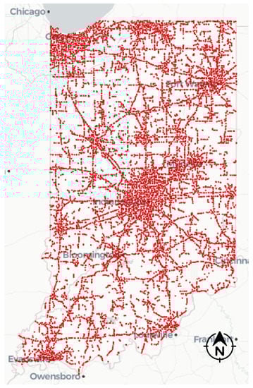
Figure 1.
More than 1.5 million CV data waypoints in Indiana between 12:00 p.m. and 12:05 p.m. on Sunday, 6 March 2022.
4.2. High-Resolution Rapid-Refresh (HRRR) Data
HRRR provides hourly weather parameter information for every 3-by-3 km spatial boundary, hereafter referred to as the HRRR grid. It provides information about precipitation rate or rain intensity, temperature conditions, visibility, wind speeds, and solar flux values, along with timestamp and location identification. Table 1 shows the rain categorization as laid out by the United States Geological Survey (USGS) [46] based on precipitation rate values.

Table 1.
Categorization of precipitation rate by USGS.
4.3. Integration of CV Data and HRRR Data
CV trajectory data was geospatially mapped within each HRRR grid to define a trip starting and ending inside the spatial boundaries. Figure 2a shows an example HRRR grid along I-65 in Indiana. Callout h refers to the boundary of the HRRR grid. Callouts i and ii indicate start mile marker (MM) 181.3 and end MM 183.2 of interstates within this HRRR grid in the northbound (NB) direction and vice versa for the southbound (SB) direction. Figure 2b shows an example CV dataset within this grid going NB for a one-hour period between 1 p.m. and 2 p.m. on 14 May 2022. The vertical axis shows the mile marker along the interstate and the horizontal axis shows the hour of the day. Individual dots represent waypoints color coded by speed. Waypoints from the same trajectory identifier are connected and shown by underlying lines. Each of these individual trajectory identifiers within the same HRRR grid and one-hour time bin is defined as a trip record. The average speed for each trip record is then calculated using all the waypoints along the trajectory within the grid. The average is then associated with the weather data attributes from HRRR for the same hour. The method is repeated for all rainstorm events in 2021 and 2022.
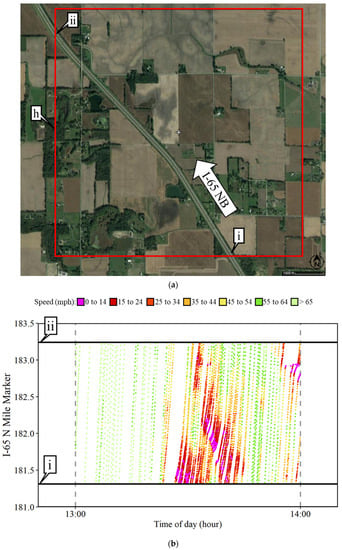
Figure 2.
Visualization of CV trajectories spanning one HRRR block for one hour on 14 May 2022, along I-65 northbound direction from MM 181.3 to MM 183.2. (a) HRRR data grid (b) Individual CV data waypoints color coded by speed bin within HRRR data grid.
4.4. Dataset
Several rainstorm events were selected along Indiana interstates I-65, I-70, and I-74 in 2021 and 2022 to build the dataset. HRRR data consisted of categorical variables that are used for filtering rainstorm events. A temporal boundary is established around each rain event, and additional two-hour buffers are included on each side of the boundary where the precipitation rate was zero. The following filters are applied:
- Exclusion of any storm events with snow or ice pellets.
- Exclusion of work zone regions (recurring congestion).
- Exclusion of incident-related traffic congestion.
- Exclusion of periods where no rain condition was experienced at all.
Additional manual screening of spatial boundaries was essential to avoid any external factors that are affecting motorists’ traffic speed. Table 2 shows the list of all rainstorm events with information about interstates, mile markers, and time ranges. A total of 562 h were selected across 42 unique days. A total of 8397 mile-hours were analyzed during this study. More than 0.3 million trip records were gathered from these rainstorm events.
Table 2.
Summary of rainstorm events over 42 unique days on Indiana interstates.
5. Explanatory Variables
5.1. Free Flow Speed Estimation
For each trip record, free flow speed () is defined as the average speed of all trips around a four-hour time window on either side of the trip start time with zero precipitation rate value within the same HRRR grid location. For example, free flow speed for the first trip record that started around 1:00 p.m. shown in Figure 2b is calculated using the average speed estimation of the trips between 9:00 a.m. and 5:00 p.m. with zero precipitation rate value on the same day within the same HRRR grid (Figure 2a).
For any trip record with the start time as within HRRR grid g, free flow speed is calculated as given in Equation (1).
where is the speed for trip record at time within the same HRRR grid g such that belongs to no rain event set and is within and hours. It was defined to estimate the free-flowing condition speed that is location-specific and time of the day relevant instead of assuming a constant value. The speed limit on the interstate was 70 mph. For 83% of the trip records across all events, the free flow speed was within the range of 65 to 75 mph when no rain was experienced.
5.2. Speed Reduction
For each trip record, if the average speed is lower than the estimated free flow speed, the difference is calculated as speed reduction for the trip record. Speed reduction was observed for 54.6% of the trip records. For each trip record with an observed speed reduction, the speed reduction percentage was estimated as the percentage decrease in average speed from the free flow speed. Six new indicator variables were created to show if the speed reductions were above thresholds of 0%, 5%, 10%, 15%, 20%, and 25%.
5.3. Descriptive Statistics
Table 3 shows the percentage of records for key indicator parameters. The nighttime indicator was defined as 1 if the start time of the trip was after 8 p.m. and before 6 a.m.. Of the 275,422 total records, 22.86% were observed during nighttime conditions. Among different rain categories, no rain conditions had the highest percentage of records (44.8%) followed by moderate rain (34.5%), slight rain (11.3%), heavy rain (5.7%), and very heavy rain (3.7%). Speed reduction was observed for more than half of the dataset (54.57%) but only 3.35% of the trip records experienced more than 25% of speed reduction. Figure 3 shows the histogram plot of continuous variables. The maximum precipitation rate value observed was 92.16 mm/h with an overall mean of 1.55 mm/h. The precipitation rate was mostly observed near 0 with a decreasing frequency for higher rain intensity values (Figure 3a). Wind speed ranged from 0.05 to 14.33 m/s (Figure 3b) with a mean of 4.07 m/s. Temperature values varied between 23.21 °F and 86.71 °F. Two clear peaks were observed on the histogram plot for temperature (Figure 3c) around 56 °F and 70 °F indicatives of daytime and nighttime conditions, respectively. HRRR data also provided information about visibility in meters. Figure 3d shows the histogram plot for visibility. Mean visibility during daytime was 14,171 m which was reduced to 12,450 m during nighttime.
Table 3.
Percent of records for key indicator parameters.
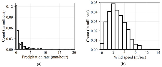
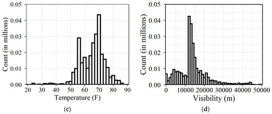
Figure 3.
Histogram plot for key continuous parameters. (a) Histogram of precipitation rate (b) Histogram of wind speed (c) Histogram of temperature (d) Histogram of visibility.
5.4. Directional Wind Estimation
Alongside the intensity of rain, wind speed, and its directions are also hypothesized to influence traffic speeds. A qualitative example described later in Figure 6 shows that wind direction had impacted one direction of travel significantly more than another along the same stretch of interstate. HRRR data provides the wind in meteorological wind directions [47]. It is important to superimpose the direction with respect to the route as motorists experience different effects from the wind blowing opposite to the direction of the travel (headwind) or with the direction (tailwind). Figure 4 shows the methodology used to compute the components of wind in four different directions. Callout r denotes the heading of the route, i.e., the direction of travel. Callout w denotes the wind-blowing direction. The components of wind are resolved in four directions shown by callouts i (headwind), ii (wind blowing from right), iii (tailwind), and iv (wind blowing from left). For example, wind shown in Figure 4 has a headwind component (denoted by ) and wind blowing from the right component (denoted by ). The other two components will be zero in this case. Depending on the direction of the blowing wind, there will always be at least two components absent. Directional wind components were estimated from all trip records.
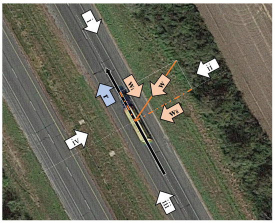
Figure 4.
Directional wind components with respect to the route or travel direction.
6. Methodology—Filtering Technique
Among the trip records generated initially, several of the records are filtered using the following techniques for data cleaning purposes. Figure 5 shows the distribution of average speed from 302,178 trip records. Callout i points to the outlier trip records with average speeds closer to 0 mph due to ramps within the HRRR grid. These accounted for 0.76% of the trip records, were considered outliers, and were removed from the analysis.
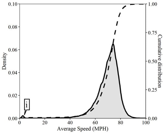
Figure 5.
Average speed distribution.
Any trips with fewer than two waypoints are also removed from the analysis. Any trips found to be trip chaining inside the HRRR grid are removed, i.e., if the time difference between the first and last recorded waypoint within the grid is more than the estimated time to traverse the section of the interstate within the grid at the lowest recorded speed for the trip. After data cleaning, 275,422 trip records remained from the initial total of 302,178. Further, a qualitative and quantitative approach was utilized to study the impact of rain intensity on traffic speeds.
7. Qualitative Approach—Case Study along I-65
Figure 6 shows a qualitative example of the impact of precipitation rate observed from HRRR data on traffic speeds along I-65 on 8 July 2021. Figure 6a,b show a spatial-temporal heatmap of traffic speed from CV data color coded by speed bins for 55 miles of the I-65 section from MM 115 to MM 170 for NB and SB, respectively. The horizontal axis represents the time of the day and the vertical axis shows the mile marker location. The direction of the arrow next to the vertical axis represents the direction of travel. Figure 6c shows the precipitation rate from HRRR data provided with a temporal resolution of one hour. The rainstorm was moving SB starting around 6:00 a.m. near MM 170 and reaching MM 115 in six hours around noon. It can be estimated that the storm was moving SB at a speed of approximately 9 mph. Traffic speeds were observed to be impacted in orange (35 to 44 mph) and in red (25 to 34 mph) in both NB and SB directions [48]. However, it can be seen that traffic in the SB direction (Figure 6b) was adversely impacted compared to NB (Figure 6a).
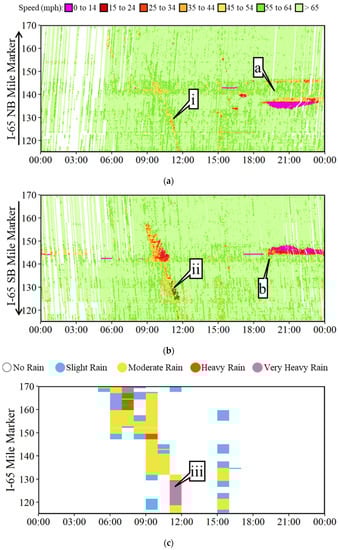
Figure 6.
Qualitative example of the impact of rain and wind direction on traffic speeds on 8 July 2021. (a) Traffic speeds from CV data along I-65 NB direction (b) Traffic speed from CV data along I-65 SB direction. (c) Precipitation rate from HRRR data along I-65.
Particularly, an hour of very heavy rain (>8 mm/h) between 11:00 a.m. and noon shown by callout iii from MM 120 to MM 130 impacted SB travel severely (callout ii) however NB traveling traffic was less impacted (callout i). Though the rain intensities were the same as it was the same stretch of the interstate, the direction of the wind was opposite for SB traffic (headwind) and in the direction (tailwind) for NB traffic. This example qualitatively confirms that along with precipitation, wind speed also has an effect on traffic speeds during rainstorm events. Figure 7 shows the ITS camera images along I-65. Camera image from MM 126.3 at 10:36 a.m. (Figure 7a) shows no sign of rain, at 11:12 a.m. (Figure 7b) very heavy rain is observed and at 12:06 p.m. (Figure 7c) the rain is cleared. Camera images confirm the ground information provided by HRRR data.
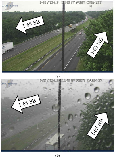
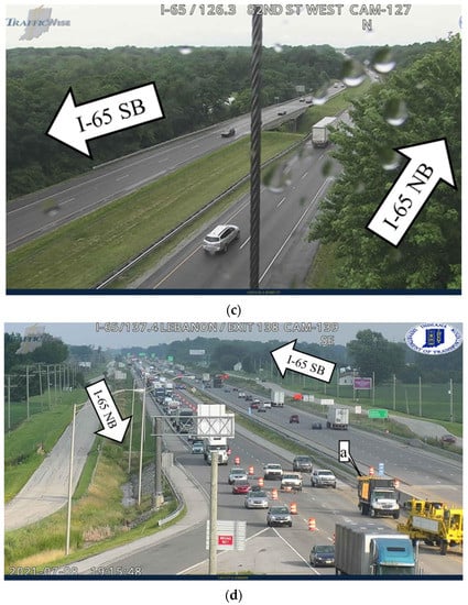
Figure 7.
ITS Camera images along I-65 MM 126.3 at similar locations shown by callout i, ii, and iii in Figure 6 and MM 138. (a) Before very heavy rain at 10:36 a.m. at MM 126.3 (b) During very heavy rain at 11:12 a.m. at MM 126.3 (c) After very heavy rain at 12:06 p.m. at MM 126.3 (d) Camera image of work zone operation at 7:15 p.m. at MM 138.
Around MM 140, traffic speeds were observed to be congested with back-of-queue traffic in both directions of travel shown by callouts a and b in Figure 6 due to work zone operations. The camera image from MM 138 at 7:15 p.m. confirms the active work zone deployment and congested traffic (callout a) shown in Figure 7d. In order to eliminate any such external factors affecting traffic speeds, all rainstorm cases were manually pruned to restrict temporal and spatial boundaries (Table 2) as explained in the data collection section.
8. Quantitative Approach
8.1. Aggregate Analysis
Figure 8 shows the density and cumulative density of average speed by precipitation rate categories as defined in Table 1 for all 275,244 trip records. It can be clearly observed that speeds lowered (shifted to the left) with increasing rain intensity category. Vertical dotted lines shown in Figure 8a represent the mean value color coded for the respective categories. The density distribution was left-skewed for all categories. Horizontal lines in Figure 8b show the first quartile (25th percentile), second quartile/median (50th percentile), and third quartile (75th percentile) respectively from bottom to top. The cumulative distribution shows a wider gap at the first quartile but a tighter fit at the third quartile between the categories, indicating an extended lower speed tail for higher precipitation rate categories due to driver behavior variability in inclement conditions.
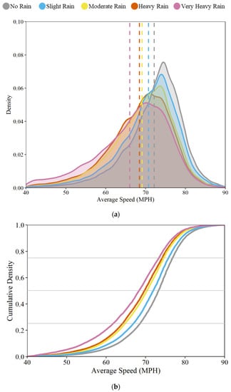
Figure 8.
Average speed distribution for various precipitation rate categories. (a) Density distribution with median speeds (dotted line) (b) Cumulative density distribution.
Table 4 summarizes speed statistics for each of these categories. Mean speed was 72.05 mph during no rain conditions which decreased up to 66 mph in very heavy rain. It decreased only by 1.93% in slight rain, 4.19% in moderate rain, 5.04% in heavy rain, and 8.40% in very heavy rain conditions. Interquartile range (IQR), i.e., third quartile minus first quartile increased with increasing precipitation rate, suggesting the driver speed selection during rainstorms increased in variability. Figure 9 shows a box-whisker plot of average speeds in different rain categories. The bottom line represents the 25th percentile, the center line 50th percentile/median, and the top line 75th percentile of average speeds for each of the categories. Black dots denote the mean of average speeds.
Table 4.
Summary of speed impacted by precipitation rate categories.
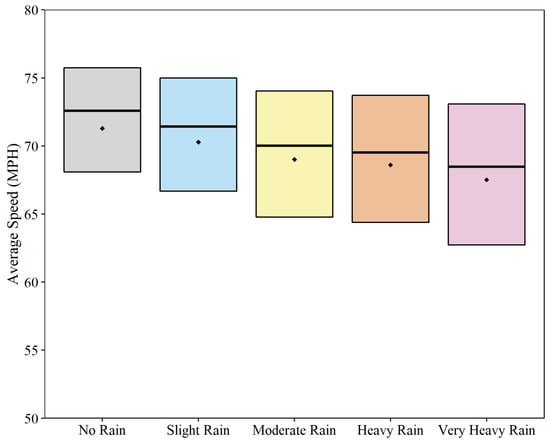
Figure 9.
Comparison of average speeds by USGS precipitation rate categories.
8.2. Disaggregate Analysis
The aggregate analysis above indicates the impact of precipitation rate on interstate travel speeds by combining all trip records together within each precipitation intensity category. However, there may exist speed variations across different HRRR grids or geolocations due to other environmental nuances, such as temperature, visibility, wind speed, and direction. A less aggregated approach is required to capture the complex relationship between speed reduction and environment-based variables. Instead of aggregating speed profiles from five rain categories, weather-related variables described in Table 3 and Figure 3 were incorporated in each trip record by spatial-temporally matching HRRR weather grids with CV data. Trip records along with weather-related explanatory variables enable us to delineate the adverse weather impact on individual drivers’ speed selection behavior in a more discretized way.
As noted in Table 3, a speed reduction behavior has a binary outcome: reduced speed or greater than equal to the estimated free-flowing speed . The response (dependent) variable is an event if speed reduction percentage is greater than the threshold, . Six levels of speed reduction thresholds are introduced: . Six separate logit models were developed corresponding to each of the speed reduction levels. The estimation results of six logit models are shown in Table 5. The probability of speed reduction above the defined threshold is given by Equation (2).
where denotes that a speed reduction is observed above the threshold, represents the matrix of explanatory variables, and represents the coefficients. Along with the estimated coefficient information, Table 5 also presents the percent-correct prediction for each of the six models. First, the predicted/replicated response is calculated as given in Equation (3).
where denotes the explanatory variables. represents the estimated coefficients in Table 5. The replicated response is then compared to the actual value of the response variable . Thus, accuracy or percent-correct prediction is calculated as the percent of the replicated response that matches the actual response. It is important to note that this includes both and responses. Model 1 had an accuracy of only 54.96%; however, the accuracy increased to 96.63% for Model 6. It is also important to note that with an increasing threshold of speed reduction, the number of trip records above that threshold also decreased, i.e., type is decreased as shown on Table 3. Models are more accurate in correctly predicting the response variable for higher speed reduction percentages compared to lower reductions.
Table 5.
Estimation results of six logit models.
8.3. Impact of Precipitation Intensity on Speeds
All coefficients of precipitation rate among the six levels of speed reductions are positive (Table 5), which means the increase in precipitation rate will increase the likelihood of speed reductions. In other words, it confers with the hypothesis that an increase in precipitation rate will increase the probability of speed reduction above the defined threshold. Additionally, in logistic regression, the odds ratio is defined as given in Equation (4).
where, represents the probability of , represents the probability of , represents the coefficient of intercept, represents the estimated coefficients listed in Table 5, and represents the explanatory variables.
For Model 2, the precipitation rate has the maximum estimated coefficient (0.0565 in Table 5). Based on Equation (4), the estimated coefficients of precipitation rate indicates that the odds ratio of reducing speed within 10% is i.e., 1.058 times higher for drivers if the precipitation rate is increased by 1 mm/h. Equivalently, a 5.8% increase in the probability of speed reduction is estimated with the increase of precipitation rate by 1 mm/h.
8.4. Impact of Nighttime Conditions
In addition, the night variable has positive estimated coefficients in the six models, which indicates that during nighttime conditions, drivers are more likely to operate at lower speeds. Based on Equation (4), the estimated coefficients (0.609 in Table 4) of driving at night indicates that the odds of reducing speed by 15% are i.e., 1.838 times higher for drivers during nighttime conditions compared to daytime conditions. On average, among all the models, the speed reduction is greater during nighttime conditions compared to daytime conditions by a factor of 1.68.
8.5. Impact of Wind
All coefficients of tailwind and wind blowing right for six models are significant and negative (Table 5), which means the increase in these will decrease the likelihood of speed reductions. Cross-directional wind blowing left was not significant and hence not included in the final model. Recall that callout iii in Figure 4 represents the direction of a tailwind which is defined as a wind blowing in the direction of travel of a vehicle. The tailwind had a subdued impact on speed reduction.
However, a headwind blowing opposite of the direction of travel will intuitively increase the likelihood of a speed reduction, up to a certain point. From Table 5, the headwind does have positive coefficients in Model 1 and Model 2, which means the increase in headwinds will increase the probability of speed reduction. Yet, for a higher level of speed reduction, the effect of headwind is less significant for Model 3 (>10%) and becomes negative for Models 4, 5, and 6 (>15%, >20%, and >25%). The headwind was found to have a positive significant impact of only up to a 10% speed reduction. A plausible explanation is that a greater than 15% speed reduction is a considerably large speed reduction, which may not be commensurate with the intensity of headwinds experienced across the 42 storms. Hence, it is reasonable to hypothesize that the marginal effect of headwinds will not be greater than a 10% reduction in speed.
A qualitative example of the effect of tailwind and headwind is also shown in Figure 6. The impacts of precipitation rate on the NB direction from callout i and the SB direction from callout ii are disproportional. Traffic from the NB direction is less influenced by the precipitation rate than the SB direction. This is because traffic from the NB direction experienced a tailwind, and traffic from the SB direction experienced a headwind. Combining qualitative and quantitative results connected the relationship between driver intuition, speed, and weather data.
8.6. Impact of Temperature
The temperature had a positive impact on the likelihood of speed reductions. However, the magnitude was small, indicating only a 0.8% increase in the probability of speed reduction in the case of Model 1 when the temperature was increased by 1 °F. This is the opposite of the expected behavior, though the magnitude of impact is small.
8.7. Impact of Visibility
Visibility was observed to be a significant factor in logit models. An interaction variable was used in the final model to understand the impact due to daytime visibility and nighttime visibility separately. Both factors, daytime, and nighttime visibility coefficients, were negative, suggesting a decrease in the likelihood of speed reduction with an improvement in visibility. The absolute magnitude of the daytime visibility coefficient was greater than the nighttime visibility coefficient. For model 1, 1000 m of improvement in visibility reduces the probability of speed reduction by 2.19% during daytime and only by 0.62% during nighttime.
8.8. Probability of Speed Reductions
Figure 10 shows the probability of speed reduction above the percentage thresholds for varying precipitation rate values during day and night conditions. The logit model was modified to include only the precipitation rate and nighttime indicator variable for this purpose. The probability of reduction of speed above a certain threshold is estimated using Equation (2). The probabilities at zero precipitation rate values show the stochastic variation in speeds under normal/no rain conditions. The probability of speed reduction increased with the increase in precipitation rate values. However, the probability of speed reduction decreased as the reduction threshold increased at any given precipitation rate. The impact of precipitation rate during night conditions (Figure 10b) was severe compared to during daytime (Figure 10a) observed from an upward shift in the probabilities plot. This can provide helpful guidance to agencies and automobile manufacturers to understand the likelihood of speed reductions for a given rain intensity during day or night conditions.
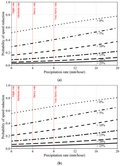
Figure 10.
Probability of speed reduction above threshold percentages at different precipitation rate values during day and night conditions. (a) Day conditions (from 6 a.m. to 8 p.m.) (b) Night conditions (from 8 p.m. to 6 a.m.).
9. Conclusions
This paper used CV data and NOAA’s HRRR weather data to observe and analyze the impact of rainstorms on interstate travel speeds. By integrating HRRR data and CV trip records spatially and temporally, this study collected 275,422 trip records during no rain, slight rain, moderate rain, heavy rain, and very heavy rain conditions over 42 days in 2021 and 2022.
First, a qualitative analysis using the case study on I-65 shows that speed impacted in both directions of travel was spatially and temporally matched with precipitation data during rainstorms. It was also noted that the impact on the SB direction of travel was significantly higher than the NB direction due to the effect of wind and its direction. Moreover, an aggregate analysis of the adverse impact of rain intensity on interstate travel speeds showed average speeds decreased by 1.93% in slight rain, 4.19% in moderate rain, 5.04% in heavy rain, and 8.40% in very heavy rain compared to the average speed of 72.05 mph during no rain conditions. Finally, a disaggregate analysis of the speed reduction probability is investigated using logit models. Estimation results indicated that a maximum of 5.8% increase in the probability of speed reduction is estimated with the increase of precipitation rate by 1 mm/h. The headwind was found to have a significant positive impact of only up to 10% speed reduction. The inclement weather impact on individual speed reduction is greater during nighttime conditions compared to daytime conditions by a factor of 1.68 across all speed reduction categories.
Both aggregate analysis and disaggregate analysis in this paper enable agencies and automobile manufacturers to answer the question about the intensity of rain it takes to begin impacting traffic speeds. Proactive measures such as providing advance warnings that improve the situational awareness of motorists and enhance roadway safety should be considered during very heavy rain periods, wind events, and daylight conditions.
Author Contributions
The authors confirm their contribution to the paper as follows: study conception and design: D.M.B., H.L. and R.S.S.; data collection: H.L., R.S.S. and Y.Z.; analysis and interpretation of results: R.S.S. and Y.Z.; draft manuscript preparation: R.S.S. and Y.Z. All authors have read and agreed to the published version of the manuscript.
Funding
This research was funded by the Indiana Department of Transportation, grant number SPR-4536.
Data Availability Statement
Not applicable.
Acknowledgments
Connected vehicle trajectory data between March 2021 and June 2022 used in this study was provided by Wejo Data Services, Inc., Manchester, England. The contents of this study reflect the views of the authors, who are responsible for the facts and the accuracy of the data presented herein and do not necessarily reflect the official views or policies of the sponsoring organizations. These contents do not constitute a standard, specification, or regulation.
Conflicts of Interest
The authors declare no conflict of interest.
References
- Wei-li, W. Analysis on Driver’s Driving Workload in Different Weather Conditions. J. Beijing Univ. Technol. 2011, 37, 540. [Google Scholar]
- Kilpeläinen, M.; Summala, H. Effects of weather and weather forecasts on driver behaviour. Transp. Res. Part F Traffic Psychol. Behav. 2007, 10, 288–299. [Google Scholar] [CrossRef]
- How Do Weather Events Impact Roads? Federal Highway Administration: Washington, DC, USA, 2020.
- Kyte, M.; Khatib, Z.; Shannon, P.; Kitchener, F. Effect of Weather on Free-Flow Speed. Transp. Res. Rec. J. Transp. Res. Board 2001, 1776, 60–68. [Google Scholar] [CrossRef]
- Zhang, J.; Song, G.; Gong, D.; Gao, Y.; Yu, L.; Guo, J. Analysis of rainfall effects on road travel speed in Beijing, China. IET Intell. Transp. Syst. 2018, 12, 93–102. [Google Scholar] [CrossRef]
- Wang, P.; Zhang, Y.; Wang, S.; Li, L.; Li, X. Forecasting Travel Speed in the Rainfall Days to Develop Suitable Variable Speed Limits Control Strategy for Less Driving Risk. J. Adv. Transp. 2021, 2021, 6637584. [Google Scholar] [CrossRef]
- Akin, D.; Sisiopiku, V.; Skabardonis, A. Impacts of Weather on Traffic Flow Characteristics of Urban Freeways in Istanbul. Procedia Soc. Behav. Sci. 2011, 16, 89–99. [Google Scholar] [CrossRef]
- Rahman, A.; Lownes, N.E. Analysis of rainfall impacts on platooned vehicle spacing and speed. Transp. Res. Part F Traffic Psychol. Behav. 2012, 15, 395–403. [Google Scholar] [CrossRef]
- Zhang, W.; Li, R.; Shang, P.; Liu, H. Impact Analysis of Rainfall on Traffic Flow Characteristics in Beijing. Int. J. Intell. Transp. Syst. Res. 2019, 17, 150–160. [Google Scholar] [CrossRef]
- Ahmed, M.M.; Ghasemzadeh, A. The impacts of heavy rain on speed and headway Behaviors: An investigation using the SHRP2 naturalistic driving study data. Transp. Res. Part C Emerg. Technol. 2018, 91, 371–384. [Google Scholar] [CrossRef]
- Khan, N.; Das, A.; Ahmed, M.M. Non-Parametric Association Rules Mining and Parametric Ordinal Logistic Regression for an In-Depth Investigation of Driver Speed Selection Behavior in Adverse Weather using SHRP2 Naturalistic Driving Study Data. Transp. Res. Rec. J. Transp. Res. Board 2020, 2674, 101–119. [Google Scholar] [CrossRef]
- Rakha, H.; Arafeh, M.; Park, S. Modeling Inclement Weather Impacts on Traffic Stream Behavior. Int. J. Transp. Sci. Technol. 2012, 1, 25–47. [Google Scholar] [CrossRef]
- Smith, B.L.; Byrne, K.G.; Copperman, R.B.; Hennessy, S.M.; Goodall, N.J. An investigation into the impact of rainfall on freeway traffic flow. In Proceedings of the 83rd Annual Meeting of the Transportation Research Board, Washington, DC, USA, 11 January 2004. [Google Scholar]
- Prokhorchuk, A.; Mitrovic, N.; Muhammad, U.; Stevanovic, A.; Asif, M.T.; Dauwels, J.; Jaillet, P. Estimating the Impact of High-Fidelity Rainfall Data on Traffic Conditions and Traffic Prediction. Transp. Res. Rec. J. Transp. Res. Board 2021, 2675, 1285–1300. [Google Scholar] [CrossRef]
- Lam, W.H.K.; Tam, M.L.; Cao, X.; Li, X. Modeling the Effects of Rainfall Intensity on Traffic Speed, Flow, and Density Relationships for Urban Roads. J. Transp. Eng. 2013, 139, 758–770. [Google Scholar] [CrossRef]
- Billot, R.; el Faouzi, N.-E.; de Vuyst, F. Multilevel assessment of the impact of rain on drivers’ behavior: Standardized methodology and empirical analysis. Transp. Res. Rec. 2009, 2107, 134–142. [Google Scholar] [CrossRef]
- Qiu, L.; Nixon, W.A. Effects of Adverse Weather on Traffic Crashes. Transp. Res. Rec. J. Transp. Res. Board 2008, 2055, 139–146. [Google Scholar] [CrossRef]
- Zhang, C.-B.; Wan, P.; Mei, Z.-H.; Zhang, P.-L. Traffic flow characteristics and models of freeway under rain weather. Wuhan Ligong Daxue Xuebao J. Wuhan Univ. Technol. 2013, 35, 63–67. [Google Scholar]
- Ali, E.M.; Ahmed, M.M.; Yang, G. Normal and risky driving patterns identification in clear and rainy weather on freeway segments using vehicle kinematics trajectories and time series cluster analysis. IATSS Res. 2021, 45, 137–152. [Google Scholar] [CrossRef]
- Ghasemzadeh, A.; Hammit, B.E.; Ahmed, M.M.; Young, R.K. Parametric Ordinal Logistic Regression and Non-Parametric Decision Tree Approaches for Assessing the Impact of Weather Conditions on Driver Speed Selection Using Naturalistic Driving Data. Transp. Res. Rec. J. Transp. Res. Board 2018, 2672, 137–147. [Google Scholar] [CrossRef]
- Faria, M.V.; Baptista, P.C.; Farias, T.L.; Pereira, J.M.S. Assessing the impacts of driving environment on driving behavior patterns. Transportation 2020, 47, 1311–1337. [Google Scholar] [CrossRef]
- Zhang, X.; Chen, M. Quantifying the Impact of Weather Events on Travel Time and Reliability. J. Adv. Transp. 2019, 2019, 8203081. [Google Scholar] [CrossRef]
- Snowden, R.J.; Stimpson, N.; Ruddle, R.A. Speed perception fogs up as visibility drops. Nature 1998, 392, 450. [Google Scholar] [CrossRef] [PubMed]
- Broughton, K.L.; Switzer, F.; Scott, D. Car following decisions under three visibility conditions and two speeds tested with a driving simulator. Accid. Anal. Prev. 2007, 39, 106–116. [Google Scholar] [CrossRef] [PubMed]
- Rahman, S.; Abdel-Aty, M.; Wang, L.; Lee, J. Understanding the Highway Safety Benefits of Different Approaches of Connected Vehicles in Reduced Visibility Conditions. Transp. Res. Rec. J. Transp. Res. Board 2018, 2672, 91–101. [Google Scholar] [CrossRef]
- Das, A.; Ahmed, M.M. Exploring the effect of fog on lane-changing characteristics utilizing the SHRP2 naturalistic driving study data. J. Transp. Saf. Secur. 2021, 13, 477–502. [Google Scholar] [CrossRef]
- Das, A.; Ghasemzadeh, A.; Ahmed, M.M. Analyzing the effect of fog weather conditions on driver lane-keeping performance using the SHRP2 naturalistic driving study data. J. Saf. Res. 2019, 68, 71–80. [Google Scholar] [CrossRef]
- Das, A.; Ahmed, M.M.; Ghasemzadeh, A. Using trajectory-level SHRP2 naturalistic driving data for investigating driver lane-keeping ability in fog: An association rules mining approach. Accid. Anal. Prev. 2019, 129, 250–262. [Google Scholar] [CrossRef] [PubMed]
- Yan, X.; Li, X.; Liu, Y.; Zhao, J. Effects of foggy conditions on drivers’ speed control behaviors at different risk levels. Saf. Sci. 2014, 68, 275–287. [Google Scholar] [CrossRef]
- McCann, K.; Fontaine, M.D. Assessing Driver Speed Choice in Fog with the Use of Visibility Data from Road Weather Information Systems. Transp. Res. Rec. J. Transp. Res. Board 2016, 2551, 90–99. [Google Scholar] [CrossRef]
- Khan, N.; Ghasemzadeh, A.; Ahmed, M. Investigating the Impact of Fog on Freeway Speed Selection using the SHRP2 Naturalistic Driving Study Data. Transp. Res. Rec. J. Transp. Res. Board 2018, 2672, 93–104. [Google Scholar] [CrossRef]
- Shabarek, A.; Chien, S.; Hadri, S. Deep Learning Framework for Freeway Speed Prediction in Adverse Weather. Transp. Res. Rec. J. Transp. Res. Board 2020, 2674, 28–41. [Google Scholar] [CrossRef]
- Brooks, J.O.; Crisler, M.C.; Klein, N.; Goodenough, R.; Beeco, R.W.; Guirl, C.; Tyler, P.J.; Hilpert, A.; Miller, Y.; Grygier, J.; et al. Speed choice and driving performance in simulated foggy conditions. Accid. Anal. Prev. 2011, 43, 698–705. [Google Scholar] [CrossRef] [PubMed]
- Rakha, H.; Farzaneh, M.; Arafeh, M.; Sterzin, E. Inclement Weather Impacts on Freeway Traffic Stream Behavior. Transp. Res. Rec. J. Transp. Res. Board 2008, 2071, 8–18. [Google Scholar] [CrossRef]
- Fu, X.; Lam, W.H.; Meng, Q. Modelling impacts of adverse weather conditions on activity–travel pattern scheduling in multi-modal transit networks. Transp. B Transp. Dyn. 2014, 2, 151–167. [Google Scholar] [CrossRef]
- Agarwal, M.; Maze, T.H.; Souleyrette, R. The weather and its impact on urban freeway traffic operations. In Proceedings of the 85th Annual Meeting of the Transportation Research Board, Washington, DC, USA, 22 January 2006. [Google Scholar]
- Katz, B.; O’Donnell, C.; Donoughe, K.; Atkinson, J.E.; Finley, M.D.; Balke, K.N.; Kuhn, B.T.; Warren, D. Guidelines for the Use of Variable Speed Limit Systems in Wet Weather; Federal Highway Administration, Office of Safety: Washington, DC, USA, 2012.
- Dailey, D.J.; Washington State Transportation Commission. The Use of Weather Data to Predict Non-Recurring Traffic Congestion; Transportation Northwest Organization: Washington, DC, USA, 2006.
- Singh, H.; Kathuria, A. Analyzing driver behavior under naturalistic driving conditions: A review. Accid. Anal. Prev. 2021, 150, 105908. [Google Scholar] [CrossRef] [PubMed]
- Sakhare, R.S.; Hunter, M.; Mukai, J.; Li, H.; Bullock, D.M. Truck and Passenger Car Connected Vehicle Penetration on Indiana Roadways. J. Transp. Technol. 2022, 12, 578–599. [Google Scholar] [CrossRef]
- Sakhare, R.S.; Desai, J.; Li, H.; Kachler, M.A.; Bullock, D.M. Methodology for Monitoring Work Zones Traffic Operations Using Connected Vehicle Data. Safety 2022, 8, 41. [Google Scholar] [CrossRef]
- Sakhare, R.S.; Desai, J.C.; Mathew, J.K.; McGregor, J.D.; Bullock, D.M. Evaluation of the Impact of Presence Lighting and Digital Speed Limit Trailers on Interstate Speeds in Indiana Work Zones. J. Transp. Technol. 2021, 11, 157–167. [Google Scholar] [CrossRef]
- Sakhare, R.S.; Desai, J.C.; Mahlberg, J.; Mathew, J.K.; Kim, W.; Li, H.; McGregor, J.D.; Bullock, D.M. Evaluation of the Impact of Queue Trucks with Navigation Alerts Using Connected Vehicle Data. J. Transp. Technol. 2021, 11, 561–576. [Google Scholar] [CrossRef]
- Desai, J.; Mahlberg, J.; Kim, W.; Sakhare, R.; Li, H.; McGuffey, J.; Bullock, D.M. Leveraging Telematics for Winter Operations Performance Measures and Tactical Adjustment. J. Transp. Technol. 2021, 11, 611–627. [Google Scholar] [CrossRef]
- McNamara, M.; Sakhare, R.S.; Li, H.; Baldwin, M.; Bullock, D. Integrating crowdsourced probe vehicle traffic speeds into winter operations performance measures. In Proceedings of the Transportation Research Board 96th Annual Meeting no. 17-00161, Washington, DC, USA, 8–12 January 2017. [Google Scholar]
- USGS. Rate of Rainfall. Available online: https://water.usgs.gov/edu/activity-howmuchrain-metric.html (accessed on 14 July 2022).
- Department of Atmospheric, Oceanic, and Earth Sciences, Virginia Weather and Climate Data. Wind: U and v Components. 2014. Available online: http://colaweb.gmu.edu/dev/clim301/lectures/wind/wind-uv (accessed on 1 December 2022).
- Sakhare, R.S.; Desai, J.; Li, H.; Mathew, J.; Bullock, D. Predicting Weather Impact on Traffic Speeds Using the Multi-Radar Multi-Sensor System. In Proceedings of the 101st American Meteorological Society Annual Meeting, virtual, 1—15 January 2021; Available online: https://ams.confex.com/ams/101ANNUAL/meetingapp.cgi/Paper/382590 (accessed on 27 July 2022).
Disclaimer/Publisher’s Note: The statements, opinions and data contained in all publications are solely those of the individual author(s) and contributor(s) and not of MDPI and/or the editor(s). MDPI and/or the editor(s) disclaim responsibility for any injury to people or property resulting from any ideas, methods, instructions or products referred to in the content. |
© 2023 by the authors. Licensee MDPI, Basel, Switzerland. This article is an open access article distributed under the terms and conditions of the Creative Commons Attribution (CC BY) license (https://creativecommons.org/licenses/by/4.0/).