Abstract
Receiving appropriate forecast accuracy is important in many countries’ economic activities, and developing effective and precise time series model is critical issue in tourism demand forecasting. In this paper, fuzzy rule-based system model for hotel occupancy forecasting is developed by analyzing 40 months’ time series data and applying fuzzy c-means clustering algorithm. Based on the values of root mean square error and mean absolute percentage error which are metrics for measuring forecast accuracy, it is defined that the model with 7 clusters and 4 inputs is the optimal forecasting model for hotel occupancy.
1. Introduction
Tourism is mentioned as one of the most significant economic fields over the last two decades: its ranking in world trade is second only to oil, which sets it apart from other economic fields. Nowadays, making a reasonable decision, especially under uncertain circumstances, is necessary in the field of tourism. Promotion in the tourism sector would be simpler if it were possible to forecast changes in number of tourists by examining current and past tourism demands. Due to the competitive and complicated environment in the tourism sector, it is required to observe and to enhance the previous standard of performances. In the prediction of tourism demand, the importance of accuracy is undeniable; however selecting a suitable model to fit a problem is as necessary as accuracy of the results. The different tourism forecasting models have been suggested by researchers, and of course each model has superiorities as well as drawbacks.
Time series methods need only one data series, and are based on the level of complexity of the model. By combining linear autoregressive integrated moving average (ARIMA) model and nonlinear artificial neural network model, an effective hybrid methodology for time series forecasting is proposed in [1], and the experimental results show that the combined approach takes the advantages of both models and significantly improves the forecasting performance.
The time series seasonal ARIMA (SARIMA) and multivariate ARIMA (MARIMA) models are used to forecast a tourism demand in Hong Kong [2], and application of these models provides better accuracy in comparison with other time series models.
The performances of ARIMA, artificial neural networks, and multivariate adaptive regression splines forecasting models are compared to obtain the appropriate model for tourism demand in Taiwan [3]. Based on the lowest value of mean absolute percentage error (MAPE), it is confirmed that ARIMA is the more appropriate model for forecasting tourism demand.
Time series data are used to examine a performance of the forecasting accuracy of demand in Taiwanese outbound tourism [4], and the experimental results show that a combination of linear and nonlinear statistical models enables better forecasting accuracy compare to other individual models.
The forecast accuracy of tourism demand is important issue for the government in terms of planning accommodation and improving transportation infrastructure in the country. The government faces negative economic impact if accurate forecasting fails. Time series forecasting of tourism demand in Malaysia is done by using Box Jenkins model, time series regression and Holt Winters methods [5]. Holt Winters and time series regression methods show better forecasting accuracy in terms of error magnitude and directional accuracy respectively.
Backpropagation is one of the popular neural network algorithms effectively used in forecasting process. Sometimes this approach does not provide a desirable accuracy of forecasting. The methodology based on combination of backpropagation and genetic algorithms can improve a forecasting accuracy, and the parameters of back propagation algorithm are optimized to minimize the prediction error. The proposed methodology is used on series dataset to predict the foreign tourist arrivals in three cities of Indonesia [6].
This is an obvious fact that increasing tourist arrivals in country positively affects the rate of employment in both governmental and private sectors of tourism industry. Simple Regression Model (SRM) and Auto Regressive Distributed Lag Model (ARDLM) are compared in [7] to determine the optimal model for forecasting the tourism generated employment in Sri-Lanka. According to relative and absolute measurements of errors, it is justified that ARDLM is more convenient forecasting model.
Combination of biquadratic polynomial function and autoregressive model can be the useful approach on tourist arrival time series data with seasonal fluctuation [8]. The proposed approach is used for prediction of monthly tourist arrivals in Nepal.
Although classical time series models have a wide range of applications, they handle with some drawbacks: the model should be specified formally and a probability distribution needs to be assumed for data [9]; it should be examined carefully whether the time series is stationary or not, since in nonstationary case, data have a stochastic trend or have a random probability distribution which causes an inaccurate forecasting [10]; the models are mostly based on a piecewise linear function; the classical models are time consuming due to selecting and testing the proper functional form by a user among various possibilities; accurate results depend on a large amount of past data [11]; and the model construction does not rely on any economic theory, which is not helpful for policy making and planning [12].
Fuzzy time-series approach is an effective tool to overcome the above mentioned drawbacks of classical time series models. Some other advantages of fuzzy time series models can be interpreted as follows: fuzzy models are effectively applied in complex and optimization problems [13]; they have more capability in nonlinear relationship [14]; they are applicable with a small set of data; they use linguistic values instead of crisp ones; they can deal with incomplete and deficient data under unclear circumstances [15].
By using fuzzy logic theory, Song and Chissom defined the fuzzy time series for the first time and used it to design a forecasting system [16]. Traditional time series data are based on numerical values which are unreliable whereas fuzzy time series data are based on linguistic values. The use of fuzzy time series was expanded due to its potential to cope with incomplete and ambiguous data [17]. Later on there have been some modifications on Song and Chissom model, such as reducing the overload computation by enhancing the fuzzy logic relationship rules [18], and designing the system to improve prediction by integrating problem-specific heuristic knowledge [19].
The forecast accuracies of fuzzy time series and grey theory are calculated to predict the annual number of visitors to the U.S. [20]. In order to enhance the forecasting accuracy of tourism demand, a novel forecasting method by combining fuzzy c-means (FCM) algorithm and logarithm least-squares support vector regression technologies is developed [21].
While designing a system for predicting tourism demand, large fluctuation and presence of limitation in collecting historical data would be critical issues. In order to be able to deal with these issues, a system based on particle swarm optimization (PSO) and adaptive fuzzy time series is proposed to predict the number of tourists from Taiwan to the U.S. [22].
The following three fuzzy time series models are proposed for predicting the number of tourist arrivals in Taiwan: neural network (NN) based fuzzy time series model is suggested in [23] to handle and manage nonlinear data. In [24], the system is designed by combining the fuzzy time series and genetic algorithm (GA) methods. The reason of this combination is mentioned as calibrating the interval’s length and obtaining the best fuzzy interval sizes to have a minimum error. Moreover, the effect of some parameters in fuzzy time series such as population size, number of intervals and order of fuzzy time series are tested and analyzed. An adaptive fuzzy time series model is developed in [25], and the efficiency of this model is verified by obtaining small values of MAPE and RMSE errors.
There is a common agreement that there is no single forecasting method to exceed all other methods consistently to provide the best forecasting result. However by combining some methods the desirable outcome can be achieved. Therefore, in order to increase accuracy and to decrease the level of complexity and the overload of calculation in forecasting, in this paper we propose a system based on combination of FCM technique and Mamdani fuzzy rule-based system (FRBS). The main advantage of this combination is stipulated by the possibility of managing the number of linguistic rules.
2. Preliminaries
Time series. It is formally represented as follows:
where is any nonlinear function, are the values of variable in periods of time series. is a forecast value of the variable X for the period t. We need to find such a function and input number q to fulfill the condition.
where is a prediction| forecast value at a time t based on the obtained model, and is an experimental value of a variable.
Fuzzy time series. Assume be the universe of discourse such that , where is a subset of real numbers on which is fuzzy set with and . Then, the fuzzy time series on is defined by , i.e., is a collection of .
Fuzzy c-means clustering. Fuzzy clusterization (FC) is a powerful scientific tool to mine knowledge from a time series consisting lots of data. By taking into consideration the fuzziness of data in time series, the fuzzy clusterization problem for m-fuzzificator (fuzzification parameters) can be described in the following form.
Let be a set of n data or objects where , and is the set of p tuples of reals, and fuzzy c partition of the set X with is shown by a partition matrix , and . The entries of the matrix A show the ’s degree of membership that belongs to cluster j and satisfy the following properties:
- ;
- ;
- .
FCM aims to minimize the following objective function:
where , and the notation means the Euclidean distance; , where is the center of cluster j. The partition matrix would be the collection of all memberships. The power of is which is used to control the degree of fuzzy overlap.
The FCM algorithm can be described as follows:
- Step 1: Initialize .
- Step 2: Compute as follows:
- Step 3: Update as follows:
- Step 4: Compute .
- Step 5: Repeat steps 2–4 until the specified number of iterations is reached or the differences between the values of in the last two steps would be less than the minimum threshold.
FCM computes the degree of membership instead of computing the absolute membership of each to one of the clusters [26].
Fuzzy rule-based system. The classical method of rule-based system which is based on IF-THEN rules is expanded to FRBS where the conditional statements look like “IF C (condition) THEN R (restriction)“, and characterized by membership functions [27].
Mamdani type fuzzy rule-based system. This is a system with multi-inputs and single-output (MISO). In Mamdani model, the rules normally include linguistic variables which are formed as follows [28,29,30,31]:
where and y denote respectively the input and output linguistic variables, and and B denote the linguistic values of input and output linguistic variables.
Mamdani model of FRBS consists of four main components. The first component is knowledge base which consists of a rule-base including fuzzy IF-THEN rules, and a database which stores fuzzy sets.
Inference engine is another component of Mamdani model, and reasoning process is carried out upon input values and fuzzy IF…THEN rules.
The fuzzification and defuzzification interfaces are other two components of Mamdani model. The fuzzification interface is required to convert crisp input values into fuzzy values. The fuzzy values are important to be used in the process of fuzzy reasoning. The defuzzification interface performs the reverse operation of a fuzzification, and transforms fuzzy output value into crisp value.
Mamdani model is appropriate in fuzzy control applications and linguistic modeling. The drawback of this model is its unsuitability for complex problems.
3. Methodology
Methodology is based on fuzzy data mining and fuzzy approximate reasoning. Knowledge mining is based on data-driven approach. For this purpose, we use fuzzy clustering. Fuzzy clustering is performed by using FCM technique. This technique is used to find the center points and the interval of each partition in the universal set. This algorithm is applied since having an unequal size of the interval of each partition causes higher accuracy of the result. Each data point in the universal set might be in more than one cluster since the clustering is based on the value of the membership function assigned to each data point. Another advantage of using FCM is that the number of required rules will be reduced significantly. FCM causes reduction in time complexity of the procedures. As a result, there is a possibility to design a supportive system which is necessary in decision making and planning.
We obtain transparent fuzzy rule-based model which approximates a dynamical relationship between forecasted value and previous value of a time series. Approximate reasoning for calculation the forecasting value is performed by Mamdani reasoning method. The methodology is described below in details:
- Create IF…THEN rules by using FCM approach which is discussed in Section 2;
- Choose the optimal number of clusters and inputs;
- This procedure is realized by using the Fuzzy Logic Toolbox in Matlab software (R2015a, MathWorks, Natick, MA, USA);
- Use Mamdani reasoning approach to obtain the forecasted value on base of given current inputs. For this purpose, we use Fuzzy Inference System Editor (FIS Editor) in Matlab software;
- The value of fuzzy output for each rule is calculated. As implication operator the following operator is used:
- The calculated fuzzy outputs of all rules are aggregated by using max operator:
4. Numerical Example and Results
This paper aims to develop fuzzy time series model for forecasting an occupancy of one of the hotels of North Cyprus. The efficiency of this model using data (observations) on guest arrivals over 40 months, is validated and proved.
Figure 1 represents the number of guest arrivals in one of the hotels of North Cyprus over 40 months.
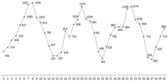
Figure 1.
Number of guest arrivals in one of the hotels of North Cyprus over 40 months.
For applying FCM clustering, we use the parameters as shown in Table 1. By using FCM, the data are clustered into clusters. The coordinates of the cluster centers with 5, 6, and 7 clusters are described in Table 2, Table 3 and Table 4, repectively.

Table 1.
Parameters of fuzzy c-means (FCM).
Table 2.
The coordinates of the cluster centers with 5 clusters.
Table 3.
The coordinates of the cluster centers with 6 clusters.
Table 4.
The coordinates of the cluster centers with 7 clusters.
After obtaining the center of each cluster, IF-THEN rules in Mamdani model should be considered. In order to have the system with high accuracy and low error value, different parameter values are tested. Mamdani-type FRBSs are designed which are based on clusters and inputs (the results for and are given in the text of the paper, and the results for and are given in Appendix A). All data are splitted into two sets called training set and testing set, and 70% of data are used for training, and other 30% of data are used for testing. To find the accuracy of each system, testing data are used. The accuracy and efficiency of each system is estimated based on the root mean square error (RMSE) and mean absolute percentage error (MAPE).
In Figure A1, the forecasting results of Mamdani-type (FRBSs) using testing data with clusters and inputs are demonstrated.
In Figure A2, the forecasting results of Mamdani-type FRBSs using testing data with clusters and inputs are demonstrated.
In Figure 2, the forecasting results of Mamdani-type FRBSs using testing data with clusters and inputs are demonstrated.
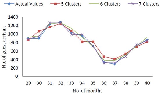
Figure 2.
Forecasting results of Mamdani-type fuzzy rule-based systems (FRBSs) using testing data with clusters and inputs.
After designing process, it is necessary to find errors for each of these models, and compare them to find the best model.
Figure A3 illustrates the actual values, forecast values and forecast errors of a time series with clusters and inputs. Figure A4 illustrates the actual values, forecast values and forecast errors of a time series with clusters and inputs. Figure 3 illustrates the actual values, forecast values and forecast errors of a time series with clusters and inputs. The forecast errors in Figure A3, Figure A4 and Figure 3 remark the performance of forecasting.
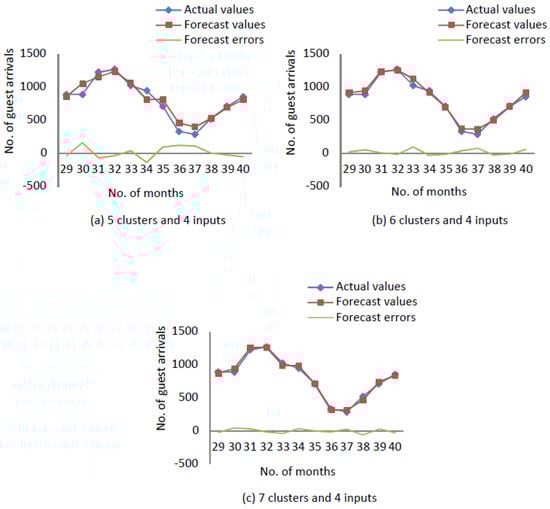
Figure 3.
Actual values, forecast values and forecast errors of a time series with clusters and inputs.
The Gaussian membership function plot and homogeneous fuzzy partitions with 7 clusters and 4 inputs are demonstrated in Figure 4.
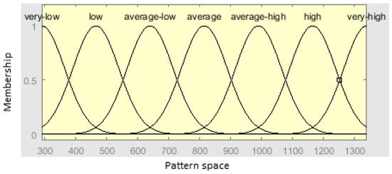
Figure 4.
Gaussian membership function plot and homogeneous fuzzy partitions with 7 clusters and 4 inputs.
The fuzzy sets and their corresponding membership functions for inputs and output of fuzzy rules are described in Figure 5.
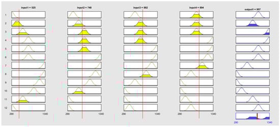
Figure 5.
Fuzzy sets and their corresponding membership functions for inputs and output of fuzzy rules.
In Mamdani-type FRBS with 7 clusters and 4 inputs, the obtained rules from testing data are represented as follows:
Rule 1: IF input1 is Gaussian(74.32, 290) and input2 is Gaussian(74.32, 465) and input3 is Gaussian(74.32, 640) and input4 is Gaussian(74.32, 815) THEN output is Gaussian(74.32, 815).
Rule 2: IF input1 is Gaussian(74.32, 290) and input2 is Gaussian(74.32, 290) and input3 is Gaussian(74.32, 465) and input4 is Gaussian(74.32, 640) THEN output is Gaussian(74.32, 990).
Rule 3: IF input1 is Gaussian(74.32, 465) and input2 is Gaussian(74.32, 640) and input3 is Gaussian(74.32, 815) and input4 is Gaussian(74.32, 815) THEN output is Gaussian(74.32, 815).
Rule 4: IF input1 is Gaussian(74.32, 640) and input2 is Gaussian(74.32, 815) and input3 is Gaussian(74.32, 815) and input4 is Gaussian(74.32, 815) THEN output is Gaussian(74.32, 1340).
Rule 5: IF input1 is Gaussian(74.32, 640) and input2 is Gaussian(74.32, 290) and input3 is Gaussian(74.32, 290) and input4 is Gaussian(74.32, 465) THEN output is Gaussian(74.32, 815).
Rule 6: IF input1 is Gaussian(74.32, 815) and input2 is Gaussian(74.32, 815) and input3 is Gaussian(74.32, 815) and input4 is Gaussian(74.32, 1340) THEN output is Gaussian(74.32, 1340).
Rule 7: IF input1 is Gaussian(74.32, 815) and input2 is Gaussian(74.32, 1340) and input3 is Gaussian(74.32, 1340) and input4 is Gaussian(74.32, 1165) THEN output is Gaussian(74.32, 990).
Rule 8: IF input1 is Gaussian(74.32, 815) and input2 is Gaussian(74.32, 815) and input3 is Gaussian(74.32, 1340) and input4 is Gaussian(74.32, 1340) THEN output is Gaussian(74.32, 990).
Rule 9: IF input1 is Gaussian(74.32, 990) and input2 is Gaussian(74.32, 640) and input3 is Gaussian(74.32, 290) and input4 is Gaussian(74.32, 290) THEN output is Gaussian(74.32, 465).
Rule 10: IF input1 is Gaussian(74.32, 1165) and input2 is Gaussian(74.32, 990) and input3 is Gaussian(74.32, 640) and input4 is Gaussian(74.32, 290) THEN output is Gaussian(74.32, 290).
Rule 11: IF input1 is Gaussian(74.32, 1340) and input2 is Gaussian(74.32, 1340) and input3 is Gaussian(74.32, 1165) and input4 is Gaussian(74.32, 990) THEN output is Gaussian(74.32, 815).
Rule 12: IF input1 is Gaussian(74.32, 1340) and input2 is Gaussian(74.32, 1165) and input3 is Gaussian(74.32, 990) and input4 is Gaussian(74.32, 640) THEN output is Gaussian(74.32, 290).
As it was mentioned, fuzzy IF-THEN rules with linguistic variables are used in Mamdani-type FRBS. The variables are expressed by such linguistic terms as “very low”, “low“, “average-low“, etc. Dealing with the linguistic terms is consistent with the vague and uncertain information. The experimental values with respect to the number of guest arrivals in the hotel include uncertainty, complexity, and nonlinearity. The traditional methods using a quantitative analysis disenable to address the matter of such imprecision and inaccuracy, and therefore, are unsuitable in these situations.
Before producing rules, the number of linguistic variables should be alleviated to a considerable size to prevent creating extra rules. With n linguistic variables, m inputs and one output, there are totally rules to be produced. However, in this research the number of rules is significantly reduced as it is depicted in Table 5 by classifying time series data.
Table 5.
Summary of performances of forecasting models
The accuracy of forecasting model is measured by applying such metrics as root mean square error (RMSE) and mean absolute percentage error (MAPE). It is obvious that the lowest values of RMSE and MAPE are the desired ones. RMSE and MAPE are calculated as follows:
where is the prediction|forecast value, and is the experimental value of ith testing data to be defined from the model, and N is the number of data used in testing.
As it can be observed from Table 5, the optimal forecasting model is the one with 7 clusters and 4 inputs with the value of RMSE equal to 31.8355 and value of MAPE equal to 4.1155%.
5. Discussion
Data-driven approach is more effective tool in fuzzy time series forecasting compare to other existing approaches. We have obtained fuzzy IF…THEN rules which are transparent, and interpretability is more suitable. By using the optimal number of IF…THEN rules, i.e., clusters from fuzzy clustering, we can get the desired accuracy of the model which is not reflected in existing time series studies. Intensive computer simulations have shown that fuzzy model with 7 clusters and 4 inputs can provide optimal solution for the forecasting problem.
6. Conclusions
Concluding above mentioned, we would like to note that data-driven approach based on fuzzy c-means technique was created to construct a fuzzy model. This model consists of 7 IF…THEN rules which include 4 antecedents. The computer experiments have proven that this model is more accurate for hotel occupancy problem. Mamdani reasoning was used for approximate reasoning which gives the forecasting value of a time series. It was defined that the measured forecasting accuracy based on the values of RMSE and MAPE which are equal to 31.8355 and 4.1155% respectively, are acceptable from point of view of hotel experts.
Author Contributions
Conceptualization and statement of the problem belong to R.A. (Rashad Aliyev); Calculation of time series processes and clusterization by using fuzzy c-means approach belong to S.S.; Reasoning processes and validity testing of the obtained results belong to R.A. (Rafig Aliyev).
Conflicts of Interest
The authors declare no conflict of interest.
Appendix A

Figure A1.
Forecasting results of Mamdani-type FRBSs using testing data with clusters and inputs.
Figure A1.
Forecasting results of Mamdani-type FRBSs using testing data with clusters and inputs.


Figure A2.
Forecasting results of Mamdani-type FRBSs using testing data with clusters and inputs.
Figure A2.
Forecasting results of Mamdani-type FRBSs using testing data with clusters and inputs.


Figure A3.
Actual values, forecast values and forecast errors of a time series with clusters and inputs.
Figure A3.
Actual values, forecast values and forecast errors of a time series with clusters and inputs.


Figure A4.
Actual values, forecast values and forecast errors of a time series with clusters and inputs.
Figure A4.
Actual values, forecast values and forecast errors of a time series with clusters and inputs.

References
- Zhang, G.P. Time series forecasting using a hybrid ARIMA and neural network model. Neurocomputing 2003, 50, 159–175. [Google Scholar] [CrossRef]
- Goh, C.; Law, R. Modeling and forecasting tourism demand for arrivals with stochastic nonstationary seasonality and intervention. Tour. Manag. 2002, 23, 499–510. [Google Scholar] [CrossRef]
- Lin, C.J.; Chen, H.F.; Lee, T.S. Forecasting Tourism Demand Using Time Series, Artificial Neural Networks and Multivariate Adaptive Regression Splines: Evidence from Taiwan. Int. J. Bus. Admin. 2011, 2, 14–24. [Google Scholar]
- Chen, K.-Y. Combining linear and nonlinear model in forecasting tourism demand. Expert Syst. Appl. 2011, 38, 10368–10376. [Google Scholar] [CrossRef]
- Nor, M.E.; Khamis, A.; Saharan, S.; Abdullah, M.A.A.; Salleh, R.M.; Asrah, N.M.; Khalid, K.; Aman, F.; Rusiman, M.S.; Halim, H.; et al. Malaysia Tourism Demand Forecasting by Using Time Series Approaches. Soc. Sci. 2016, 11, 2938–2945. [Google Scholar]
- Noersasongko, E.; Julfia, F.T.; Syukur, A.; Purwanto; Pramunendar, R.A.; Supriyanto, C. A Tourism Arrival Forecasting using Genetic Algorithm based Neural Network. Indian J. Sci. Technol. 2016, 9. [Google Scholar] [CrossRef]
- Mudiyanselage, K.; Konarasinghe, U.B. Forecasting Tourism Generated Employment in Sri Lanka: Multivariate Time Series Approach. Int. J. Res. Rev. 2018, 5, 61–67. [Google Scholar]
- Subedi, A. Time Series Modeling on Monthly Data of Tourist Arrivals in Nepal: An Alternative Approach. Nepal. J. Stat. 2017, 1, 41–54. [Google Scholar] [CrossRef]
- Hansen, J.V.; McDonald, J.B.; Nelson, R.D. Time series prediction with genetic-algorithm designed neural networks: An empirical comparison with modern statistical models. Comput. Intell. 1999, 15, 171–184. [Google Scholar] [CrossRef]
- Wang, C.-H.; Hsu, L.-C. Constructing and applying an improved fuzzy time series model: Taking the tourism industry for example. Expert Syst. Appl. 2008, 34, 2732–2738. [Google Scholar] [CrossRef]
- Shahrabi, J.; Hadavandi, E.; Asadi, S. Developing a hybrid intelligent model for forecasting problems: Case study of tourism demand time series. Knowl.-Based Syst. 2013, 43, 112–122. [Google Scholar] [CrossRef]
- Peng, B.; Song, H.; Crouch, G.I. A meta-analysis of international tourism demand forecasting and implications for practice. Tour. Manag. 2014, 45, 181–193. [Google Scholar] [CrossRef]
- Konar, A. Computational Intelligence: Principles, Techniques and Applications; Springer: Berlin, Germany, 2005. [Google Scholar]
- Hung, J.-C. A fuzzy GARCH model applied to stock market scenario using a genetic algorithm. Expert Syst. Appl. 2009, 34, 11710–11717. [Google Scholar] [CrossRef]
- Li, S.-T.; Cheng, Y.-C.; Lin, S.-Y. A FCM-based deterministic forecasting model for fuzzy time series. Comput. Math. Appl. 2008, 56, 3052–3063. [Google Scholar] [CrossRef]
- Song, Q.; Chissom, B.S. Forecasting enrollments with fuzzy time series—Part I. Fuzzy Sets Syst. 1993, 54, 1–9. [Google Scholar] [CrossRef]
- Song, Q.; Chissom, B.S. Fuzzy time series and its models. Fuzzy Sets Syst. 1993, 54, 269–277. [Google Scholar] [CrossRef]
- Chen, S.M. Forecasting enrollments based on fuzzy time series. Fuzzy Sets Syst. 1996, 81, 311–319. [Google Scholar] [CrossRef]
- Huarng, K. Heuristic models of fuzzy time series for forecasting. Fuzzy Sets Syst. 2001, 123, 369–386. [Google Scholar] [CrossRef]
- Yu, G.; Schwartz, Z. Forecasting short time-series tourism demand with artificial intelligence models. J. Travel Res. 2006, 45, 194–203. [Google Scholar] [CrossRef]
- Pai, P.-F.; Hung, K.-C.; Lin, K.-P. Tourism demand forecasting using novel hybrid system. Expert Syst. Appl. 2014, 41, 3691–3702. [Google Scholar] [CrossRef]
- Huang, Y.-L.; Horng, S.-J.; Kao, T.-W.; Kuo, I.-H.; Takao, T. A hybrid forecasting model based on adaptive fuzzy time series and particle swarm optimization. In Proceedings of the International Symposium on Biometrics and Security Technologies, Taipei, Taiwan, 26–29 March 2012; pp. 66–70. [Google Scholar]
- Huarng, K.-H.; Moutinho, L.; Yu, T.H.-K. An advanced approach to forecasting tourism demand in Taiwan. J. Travel Tour. Mark. 2007, 21, 15–24. [Google Scholar] [CrossRef]
- Sakhuja, S.; Jain, V.; Kumar, S.; Chandra, C.; Ghildayal, S.K. Genetic algorithm based fuzzy time series tourism demand forecast model. Ind. Manag. Data Syst. 2016, 116, 483–507. [Google Scholar] [CrossRef]
- Tsaur, R.-C.; Kuo, T.-C. The adaptive fuzzy time series model with an application to Taiwan’s tourism demand. Expert Syst. Appl. 2011, 38, 9164–9171. [Google Scholar] [CrossRef]
- Aliev, R.R.; Salehi, S. Implementation of fuzzy C-means clustering technique for the hotel occupancy problem. In Proceedings of the Ninth World Conference “Intelligent Systems for Industrial Automation”, WCIS-2016, Tashkent, Uzbekistan, 25–27 October 2016; pp. 14–19. [Google Scholar]
- Zadeh, L. Fuzzy sets. Inf. Control 1965, 8, 338–353. [Google Scholar] [CrossRef]
- Mamdani, E.H. Applications of fuzzy algorithm for control a simple dynamic plant. Proc. IEEE. Inst. Electr. Electron. Eng. 1974, 121, 1585–1588. [Google Scholar] [CrossRef]
- Mamdani, E.H.; Assilian, S. An experiment in linguistic synthesis with a fuzzy logic controller. Int. J. Man. Mach. Stud. 1975, 7, 1–13. [Google Scholar] [CrossRef]
- Aliev, R.A.; Aliev, R.R. Soft Computing and its Applications; World Scientific: Singapore, 2001. [Google Scholar]
- Aliev, R.A.; Fazlollahi, B.; Aliev, R.R. Soft Computing and its Applications in Business and Economics; Springer: Berlin, Germany, 2004. [Google Scholar]


© 2019 by the authors. Licensee MDPI, Basel, Switzerland. This article is an open access article distributed under the terms and conditions of the Creative Commons Attribution (CC BY) license (http://creativecommons.org/licenses/by/4.0/).