Abstract
Time series forecasting is a cornerstone of decision-making in energy and finance, yet many studies fail to rigorously analyse the underlying dataset characteristics, leading to suboptimal model selection and unreliable outcomes. This paper addresses these shortcomings by presenting a comprehensive framework that integrates fundamental time series diagnostics—stationarity tests, autocorrelation analysis, heteroscedasticity, multicollinearity, and correlation analysis—into forecasting workflows. Unlike existing studies that prioritise pre-packaged machine learning and deep learning methods, often at the expense of interpretable statistical benchmarks, our approach advocates for the combined use of statistical models alongside advanced machine learning methods. Using the Day-Ahead Market dataset from the Irish electricity market as a case study, we demonstrate how rigorous statistical diagnostics can guide model selection, improve interpretability, and improve forecasting accuracy. This work offers a novel, integrative methodology that bridges the gap between statistical rigour and modern computational techniques, improving reliability in time series forecasting.
1. Introduction
Time series forecasting has become an indispensable tool across domains such as energy, finance, healthcare, and supply chain management. As forecasting needs have evolved, so too have the models applied, with machine learning (ML) and deep learning (DL) techniques becoming increasingly prevalent. These methods excel in capturing complex patterns and processing large datasets, often achieving higher predictive accuracy compared to traditional statistical approaches. However, their widespread adoption has created a critical challenge: a tendency to overlook the intrinsic statistical properties of time series data, which can lead to misaligned models and unreliable results.
Understanding the statistical characteristics of time series data is fundamental to effective forecasting. Properties such as stationarity, autocorrelation, heteroscedasticity, multicollinearity, and correlation analysis are not only diagnostic tools but also essential for aligning models with the structural patterns of the data. Despite their importance, many studies bypass these diagnostics in favour of pre-packaged ML/DL solutions, often neglecting statistical models like Auto-Regressive Integrated Moving Average (ARIMA) and LASSO-Estimated AR (LEAR). These models serve as interpretable, robust benchmarks that can contextualise the performance of advanced methods. The absence of such benchmarks risks exaggerating the benefits of ML models, especially when residual analyses fail to detect or address issues like autocorrelation, heteroscedasticity, or structural misfit.
Furthermore, neglecting rigorous baseline testing undermines the ability to understand why models succeed or fail. Forecasting is not purely about minimising prediction error; it involves uncovering the interactions between data properties, model assumptions, and the dynamic behaviours of the underlying system. A systematic approach to time series analysis provides insights into necessary data transformations, appropriate model configurations, and iterative improvements. For instance, residual diagnostics can reveal overlooked seasonality or trends, enabling corrections that improve model interpretability.
This study bridges these gaps by proposing a systematic integration of time series diagnostics into forecasting workflows. Unlike prior work focused on performance metrics, this paper emphasises the synergy between statistical rigour and ML capabilities to improve dataset quality and model selection. Using the Day-Ahead Market (DAM) dataset as a case study, we demonstrate how a thorough time series analysis can uncover dataset nuances and refine model assumptions to deliver forecasts that are both accurate and generalisable.
2. Literature Review
Many recent studies in electricity price forecasting (EPF) adopt ML and DL approaches but fail to conduct comprehensive time series analyses, limiting their ability to select appropriate models. For instance, ref. [1] proposed a hybrid CNN-LSTM model with sensitivity analyses for predictor selection but neglected critical time series diagnostics, such as stationarity testing and autocorrelation analysis, relying instead on a basic multivariate linear regression as the statistical baseline. Similarly, ref. [2] employed a hybrid LSTM–Neural Prophet model but excluded traditional time series analysis and statistical models, undermining methodological rigour and comparative evaluation. In both cases, insufficient exploration of time series properties limits the interpretability of results, leaving their conclusions dependent on the implicit assumptions of ML models. Additionally, refs. [3,4] illustrated this trend by introducing ML/DL frameworks for EPF without incorporating time series diagnostics or statistical models as baselines, compromising the validity of their findings.
Conversely, while ML/DL methods excel in handling large, high-dimensional datasets and uncovering non-linear relationships, statistical approaches remain indispensable for their interpretability and robustness. For example, ref. [5] employ AR(FI)MA-GARCH models augmented with exogenous regressors to account for key market fundamentals, demonstrating strong performance in both point and density forecasting. Their approach showcases the advantages of leveraging domain knowledge and incorporating advanced statistical techniques for structured data. However, these studies, focusing on statistical models, overlook the potential of integrating modern ML methods, which could capture non-linear interactions to address diverse data characteristics and market dynamics.
Papers that successfully integrate statistical foundations with advanced ML/DL methods provide a promising direction for EPF research. For instance, ref. [6] employed detailed time series analyses, including stationarity diagnostics and feature selection, alongside benchmarks such as ARIMA and LEAR, to provide more comprehensive model comparisons. Similarly, ref. [7] demonstrated effective model selection through distributional neural networks, which accommodate the inherent uncertainties in electricity prices. However, their limited use of statistical diagnostics highlights opportunities for improvement in dataset evaluation. In contrast, this study takes a holistic approach by embedding rigorous time series diagnostics into workflows, ensuring that data properties guide model selection.
3. Methodology
This study employs statistical methods to preprocess and analyse time series data for accurate forecasting. Key steps include stationarity tests, diagnostics for serial correlation and heteroscedasticity, multicollinearity and correlation analysis, and a residual analysis.
3.1. Stationarity Test
In time series analysis, stationarity is a fundamental property where the statistical characteristics of a series, such as mean, variance, and autocorrelation, remain constant over time. Non-stationary data, which may exhibit trends, seasonality, or varying volatility, can lead to inaccurate and misleading forecasts. Ensuring stationarity in these datasets is fundamental to producing reliable forecasts, as forecasting techniques often assume that the data is stationary. To assess and address potential non-stationarity in time series datasets, two widely used tests were applied: the Augmented Dickey–Fuller (ADF) test, introduced in [8], and the Kwiatkowski–Phillips–Schmidt–Shin (KPSS) test, introduced in [9].
3.1.1. Augmented Dickey–Fuller Test
The ADF test is used to assess whether a time series contains a unit root, indicating non-stationarity. The ADF test evaluates the null hypothesis (), which states that it is stationary, using a model that incorporates differenced terms, a trend component, and lagged values to account for autocorrelation. The test statistic is then compared against critical values at standard significance levels; if the statistic is more negative than the critical value, the null hypothesis of non-stationarity is rejected. Applying the ADF test to time series datasets ensures that the data is suitable for further statistical modelling by either confirming stationarity or guiding the need for differencing, reducing the risk of spurious results.
3.1.2. Kwiatkowski–Phillips–Schmidt–Shin Test
The KPSS test complements the ADF test by reversing the null hypothesis and assessing trend stationarity. The KPSS model decomposes the time series into a deterministic trend, a random walk, and a stationary error term, expressed as , where is the observed series, is the intercept, represents the trend, and captures the non-stationary behaviour. If the KPSS statistic exceeds critical values, it indicates non-stationarity; values below critical thresholds support stationarity.
3.2. Serial Correlation Tests
Serial correlation, or autocorrelation, occurs when the residuals in a time series model are correlated with each other over time, which can lead to inefficient estimates, incorrect inferences, and unreliable models for time series forecasting. To address this, we employ the Least Absolute Shrinkage and Selection Operator (LASSO) model, which is well-suited for high-dimensional data. To test for serial correlation in the residuals of the LASSO model, we use the Ljung–Box test, introduced in [10], and the Breusch–Godfrey test, introduced in [11] and extended by [12]. These tests help diagnose whether any autocorrelation remains after accounting for the model’s structure, ensuring the adequacy of the forecasting models.
3.2.1. Ljung–Box Test
The Ljung–Box test assesses whether the residuals of a model are uncorrelated across multiple lags. The Ljung–Box test statistic Q is calculated as follows:
where T is the total number of observations, represents the sample autocorrelation at lag k, and m is the number of lags being tested.
3.2.2. Breusch–Godfrey Test
The Breusch–Godfrey test identifies higher-order serial correlations in residuals across multiple lags. Unlike tests limited to first-order autocorrelation, it evaluates dependencies over several periods. This is achieved by regressing the residuals from the original model on their lagged values (up to a specified lag m) and the independent variables from the model. This auxiliary regression takes the following form:
where coefficients β1, β2, …, βm represent the influence of past residuals on the current residual.
3.3. Heteroscedasticity Tests
Heteroscedasticity occurs when the variance of the residuals in a regression model are not constant across all levels of the independent variables. Addressing heteroscedasticity is important, as it violates the assumption of constant variance, a key foundation of many statistical models. If left uncorrected, heteroscedasticity can result in inefficient parameter estimates and unreliable hypothesis testing. To diagnose the presence of heteroscedasticity in the residuals, we employ two tests: the Breusch–Pagan Test [13] and the White Test [14].
3.3.1. Breusch–Pagan Test
The Breusch–Pagan Test is used to detect heteroscedasticity in the residuals of a regression model. The test involves running an auxiliary regression where the squared residuals from the original model are regressed on the independent variable vector . This auxiliary regression is expressed as follows:
where the coefficient vector measures the relationship between the variance of the residuals and independent variables, and represents the error term for the auxiliary regression.
3.3.2. White Test
The White Test is a versatile method for detecting heteroscedasticity in a regression model, without assuming any specific form of the relationship between the residual variance and the independent variables. Unlike the Breusch–Pagan Test, which tests for a linear relationship, the White Test can detect both linear and non-linear forms of heteroscedasticity. The auxiliary regression includes the independent variables, their squared terms, and interaction terms to capture potential non-linear effects:
where represents the squared residuals, denotes the independent variables, denotes their squared terms, and denotes the interaction terms capturing non-linear relationships.
3.4. Multicollinearity Tests
Multicollinearity occurs when two or more independent variables in a regression model exhibit a high degree of correlation, which can result in inflated standard errors, making coefficient estimates unreliable. This can obscure relationships between predictors and the dependent variable, leading to unstable models. Therefore, addressing multicollinearity is crucial for producing accurate, interpretable, and reliable models, reducing overfitting. To assess multicollinearity in datasets, two key diagnostic parameters are commonly employed: the Variance Inflation Factor (VIF) and the Condition Index, introduced in [15].
3.4.1. Variance Inflation Factor
The VIF measures how much the variance of a regression coefficient is inflated due to multicollinearity. It assesses the linear relationship between a predictor and the other predictors, and is calculated as follows:
where represents the proportion of variance in explained by the other predictors. A VIF above 10 generally signals problematic multicollinearity, which may require the removal or combination of predictors.
3.4.2. Condition Index
The Condition Index detects multicollinearity stemming from interactions among multiple variables. While the VIF targets individual predictors, the Condition Index evaluates overall multicollinearity using the eigenvalues of the design matrix , calculated as follows:
where is the largest eigenvalue, and is the t-th eigenvalue. A Condition Index above 30 typically indicates severe multicollinearity, suggesting that some variables may need to be removed or combined to improve model stability.
3.5. Correlation Analysis
Correlation analysis is fundamental to understanding the relationships between variables in time series datasets. By analysing the connections between each market’s predictors, correlation analysis aids in the development of accurate prediction models. This study utilises two key methods: the Pearson Correlation Coefficient [16], which measures linear relationships, and the Spearman Rank Correlation [17], assessing monotonic relationships.
3.5.1. Pearson Correlation Coefficient
The Pearson Correlation Coefficient, r, measures the strength and direction of the linear relationship between two continuous variables, defined as follows:
where and are individual data points at time t, and are the means of and y, and n is the number of observations. The coefficient r ranges from −1 to 1, with indicating a perfect positive linear relationship, indicating a perfect negative linear relationship, and indicating no linear relationship.
3.5.2. Spearman Rank Correlation
The Spearman Rank Correlation, denoted by , is a non-parametric measure that evaluates the strength and direction of the monotonic relationship between two variables. Unlike the Pearson correlation, which assesses only linear relationships, Spearman’s correlation determines how well the relationship between two variables can be described by a monotonic function. This makes it particularly useful for data that may not exhibit a linear relationship or does not follow a normal distribution. This is calculated as follows:
where represents the difference between the ranks of each pair of observations at time t, and n is the number of observations. Like r in (7), ranges from −1 to 1, with values near 1 indicating a strong positive monotonic relationship, and values near −1 indicating a strong negative monotonic relationship.
4. Experimental Evaluation
This section involves the evaluation of the DAM dataset using a rigorous selection of statistical and diagnostic techniques to investigate preprocessing for the dataset and appropriate models for forecasting the DAM price. Utilising datasets from the Irish electricity market spanning 2019 to 2022, as introduced in [18,19], the analysis focuses on a market with high curtailment rates due to surplus renewable generation during low-demand periods. Key steps include testing for stationarity, identifying temporal dependencies, and detecting serial correlation, heteroscedasticity, multicollinearity, and a residual analysis.
4.1. Stationarity
The initial ADF tests, as shown in Table 1, indicated that the DAM dataset is stationary without differencing, with highly negative test statistics and low p-values. However, the KPSS test identified non-stationarity, suggesting the presence of a trend. After differencing the data, the KPSS test confirmed that both of the DAM series became stationary.

Table 1.
ADF and KPSS test results for DAM datasets.
If the KPSS test did not confirm stationarity after differencing, further remedies, such as additional differencing or applying transformations like logarithms or de-trending via decomposition, with regular stationarity checks, were used when extending to new time periods.
4.2. Serial Correlation
The Ljung–Box test results (Table 2) for the LEAR model at lags 24, 48, 96, and 167 all show high p-values, well above 0.05, indicating no significant autocorrelation in the residuals. This suggests that the model effectively captures the temporal dependencies, and the residuals behave independently across the tested time lags. Similarly, the Breusch–Godfrey test shows no evidence of serial correlation at any of the tested lags, with all p-values above the conventional threshold. These results confirm that the DAM model adequately accounts for serial dependencies, resulting in robust and independent residuals.
Table 2.
Ljung–Box and Breusch–Godfrey test results for DAM models.
Residual diagnostics should remain a standard step when dealing with serial correlation, with fixes such as modifying the model to incorporate higher-order AR terms, or switching to models designed to handle serial correlation, such as ARIMA or state-space models.
4.3. Heteroscedasticity
The Breusch–Pagan Test (Table 3) for the DAM yielded an LM statistic of and a p-value of , rejecting the null hypothesis of homoscedasticity and indicating significant heteroscedasticity. Similarly, the White Test results (statistic = , p-value = 0.0) corroborate these findings, confirming that residual variance is not constant.
Table 3.
Breusch–Pagan and White Test results for DAM.
Heteroscedasticity in the DAM dataset, driven by demand fluctuations, price trends, and renewable variability, distorts standard errors and undermines forecasting accuracy, particularly during volatile periods like peak demand or energy surpluses. Addressing heteroscedasticity involves applying variance-stabilising transformations like logarithmic or Box–Cox methods or using heteroscedasticity-consistent regression models to ensure robust estimates. Advanced methods like GARCH further enhance resilience by explicitly modelling dynamic variance patterns, improving forecasting accuracy under market instability.
4.4. Multicollinearity
The VIF and Condition Index results (Table 4) indicate no significant multicollinearity issues. The variables Past Prices, Wind Forecast, and Demand Forecast all have VIF values close to 1, suggesting minimal correlations with other predictors. These results are corroborated by the low Condition Index values, all of which are well below the threshold of 30, indicating that the model is capable of providing both stable and reliable coefficient estimates.
Table 4.
VIF and Condition Index results for DAM.
Periodically reevaluating multicollinearity as the dataset evolves is key, and solutions include removing or combining correlated predictors and using regularisation methods like Ridge or LASSO, or principal component analysis (PCA) to reduce dimensionality.
4.5. Correlation Analysis
Pearson and Spearman Rank Correlations were calculated to assess the relationships between DAM prices and their predictors. The Pearson correlation matrix (Figure 1a) shows a moderate positive correlation () between DAM Prices and Demand Forecasts, indicating that higher demand forecasts tend to increase prices. In contrast, the correlation with Wind Forecasts is weak and negative (), suggesting minimal influence. The Spearman analysis (Figure 1b) highlights similar trends but captures additional non-linear dynamics. A stronger positive correlation () is observed between DAM Prices and Demand Forecasts, while the relationship with Wind Forecasts remains weakly negative (). A slight positive correlation () between Demand Forecasts and Wind Forecasts reflects their limited interaction. These results indicate that DAM Prices are more influenced by Demand Forecasts than Wind Forecasts, reinforcing insights from both correlation methods.
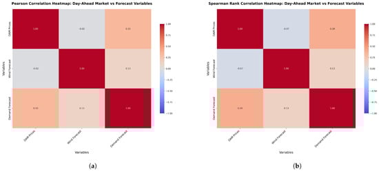
Figure 1.
Comparison of Pearson and Spearman correlation plots for the DAM prices and predictors. (a) Pearson correlation plots for the DAM prices and predictors; (b) Spearman Rank Correlation plots for the DAM prices and predictors.
If stronger correlations with wind forecasts or unexpected predictor relationships are observed, further exploratory analysis and advanced feature engineering, like polynomial or interaction terms, could capture non-linear dynamics and improve model fidelity.
4.6. Residual Analysis
Residual analysis evaluates model performance and identifies underlying issues by examining how residuals are distributed around zero. Ideally, residuals should be randomly dispersed, indicating that the model has captured the data structure well. For EPF in the DAM, residual plots assess non-linearity and heteroscedasticity, where patterns like funnels may suggest heteroscedasticity, and systematic curves may indicate non-linearity or misspecification. The residual plot for DAM (Figure 2) reveals that the LEAR model shows clustered residuals around zero, accompanied by a funnel shape, indicating both heteroscedasticity and non-linearity. Additionally, outliers suggest periods of poor model fit. In contrast, the RF model shows a more random residual dispersion around zero, reflecting a better fit but still with a few outliers at higher fitted values.
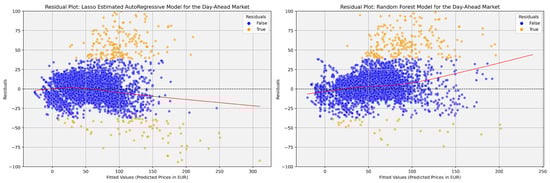
Figure 2.
Residual plots for Day-Ahead Market forecasts.
For the LEAR model, addressing heteroscedasticity and non-linearity in residuals requires either incorporating non-linear transformations or switching to non-linear or ensemble models. Detecting and managing outliers using methods such as robust regression or filtering techniques can enhance models, ensuring alignment with dataset characteristics.
5. Conclusions
This study underscores the fundamental role of time series analysis in EPF, demonstrating how rigorous statistical diagnostics provide a deeper understanding of dataset limitations and guide the selection of appropriate forecasting models. Using DAM datasets from the Irish electricity market, we conducted a comprehensive suite of tests for stationarity, autocorrelation, serial correlation, heteroscedasticity, and multicollinearity. These analyses ensured the data’s alignment with the assumptions of statistical and ML models, addressing challenges like seasonality, demand–supply fluctuations, and market volatility. Correlation analyses further refined this understanding by highlighting the moderate influence of demand forecasts on DAM prices, offering insights into the predictive power of specific variables. This analytical foundation revealed the strengths and limitations of various forecasting approaches, ensuring the selection of models that align with the dataset’s structure and market characteristics. Through this balanced integration of statistical rigour and advanced computational techniques, we demonstrate how time series analysis not only enhances model reliability and interpretability but also informs decisions about model selection. Whether opting for classical statistical methods or sophisticated ML frameworks, these insights ensure that forecasting approaches are both robust and contextually relevant for addressing the complex nature of electricity markets. Future works can work on applying these tests to new datasets (i.e., Balancing Market in [20,21]) for better model and variable selection. The code used for this analysis is available at GitHub Repository (https://github.com/ciaranoc123/Time-Series-Analysis) (access on 4 August 2025).
Author Contributions
Study conception and design: C.O. and A.V.; acquisition, analysis, creation of figures, and interpretation of data: C.O. and A.V.; drafting of manuscript: C.O., A.V. and S.P.; critical revision: C.O., A.V. and S.P. All authors have read and agreed to the published version of the manuscript.
Funding
This work was conducted with the financial support of Science Foundation Ireland under Grant Nos. 12/RC/2289-P2 and 18/CRT/6223, which are co-funded under the European Regional Development Fund. This research was partially supported by the EU’s Horizon Digital, Industry, and Space programme under grant agreement ID 101092989-DATAMITE. For the purpose of Open Access, the author has applied a CC BY public copyright license to any Author Accepted Manuscript version arising from this submission.
Institutional Review Board Statement
Not applicable.
Informed Consent Statement
Not applicable.
Data Availability Statement
The data was sourced from the SEMO (https://www.sem-o.com/) (access on 4 August 2025) and SEMOpx (https://www.semopx.com/market-data/) (access on 4 August 2025) websites, comprising historical and forward-looking data dating from 2019 to 2022. For interested readers, the data for the DAM and BM can be accessed at https://github.com/ciaranoc123/Balance-Market-Forecast (access on 4 August 2025).
Conflicts of Interest
The authors declare no conflicts of interest.
References
- Heidarpanah, M.; Hooshyaripor, F.; Fazeli, M. Daily electricity price forecasting using artificial intelligence models in the Iranian electricity market. Energy 2023, 263, 126011. [Google Scholar] [CrossRef]
- Shohan, M.J.A.; Faruque, M.O.; Foo, S.Y. Forecasting of electric load using a hybrid LSTM-neural prophet model. Energies 2022, 15, 2158. [Google Scholar] [CrossRef]
- Shi, W.; Wang, Y.F. A robust electricity price forecasting framework based on heteroscedastic temporal Convolutional Network. Int. J. Electr. Power Energy Syst. 2024, 161, 110177. [Google Scholar] [CrossRef]
- Nazir, A.; Shaikh, A.K.; Shah, A.S.; Khalil, A. Forecasting energy consumption demand of customers in smart grid using Temporal Fusion Transformer (TFT). Results Eng. 2023, 17, 100888. [Google Scholar] [CrossRef]
- Billé, A.G.; Gianfreda, A.; Del Grosso, F.; Ravazzolo, F. Forecasting electricity prices with expert, linear, and nonlinear models. Int. J. Forecast. 2023, 39, 570–586. [Google Scholar] [CrossRef]
- Kapoor, G.; Wichitaksorn, N. Electricity price forecasting in New Zealand: A comparative analysis of statistical and machine learning models with feature selection. Appl. Energy 2023, 347, 121446. [Google Scholar] [CrossRef]
- Marcjasz, G.; Narajewski, M.; Weron, R.; Ziel, F. Distributional neural networks for electricity price forecasting. Energy Econ. 2023, 125, 106843. [Google Scholar] [CrossRef]
- Dickey, D.A.; Fuller, W.A. Likelihood ratio statistics for autoregressive time series with a unit root. Econom. J. Econom. Soc. 1981, 49, 1057–1072. [Google Scholar] [CrossRef]
- Kwiatkowski, D.; Phillips, P.C.; Schmidt, P.; Shin, Y. Testing the null hypothesis of stationarity against the alternative of a unit root: How sure are we that economic time series have a unit root? J. Econom. 1992, 54, 159–178. [Google Scholar] [CrossRef]
- Ljung, G.M.; Box, G.E. On a measure of lack of fit in time series models. Biometrika 1978, 65, 297–303. [Google Scholar] [CrossRef]
- Breusch, T.S. Testing for autocorrelation in dynamic linear models. Aust. Econ. Pap. 1978, 17, 334–355. [Google Scholar] [CrossRef]
- Godfrey, L.G. Testing against general autoregressive and moving average error models when the regressors include lagged dependent variables. Econometrica 1978, 46, 1293–1301. [Google Scholar] [CrossRef]
- Breusch, T.S.; Pagan, A.R. A simple test for heteroscedasticity and random coefficient variation. Econometrica 1979, 47, 1287–1294. [Google Scholar] [CrossRef]
- White, H. A heteroskedasticity-consistent covariance matrix estimator and a direct test for heteroskedasticity. Econometrica 1980, 48, 817–838. [Google Scholar] [CrossRef]
- Snee, R.D. Regression diagnostics: Identifying influential data and sources of collinearity. J. Qual. Technol. 1983, 15, 149–153. [Google Scholar] [CrossRef]
- Pearson, K. VII. Note on regression and inheritance in the case of two parents. Proc. R. Soc. Lond. 1895, 58, 240–242. [Google Scholar] [CrossRef]
- Spearman, C. The proof and measurement of association between two things. In Studies in Individual Differences: The Search for Intelligence; Appleton-Century-Crofts: Norwalk, CT, USA, 1961. [Google Scholar]
- O’Connor, C.; Collins, J.; Prestwich, S.; Visentin, A. Electricity Price Forecasting in the Irish Balancing Market. Energy Strategy Rev. 2024, 54, 101436. [Google Scholar] [CrossRef]
- O’Connor, C.; Collins, J.; Prestwich, S.; Visentin, A. Optimising quantile-based trading strategies in electricity arbitrage. Energy AI 2025, 20, 100476. [Google Scholar] [CrossRef]
- O’Connor, C.; Prestwich, S.; Visentin, A. Conformal Prediction Techniques for Electricity Price Forecasting. In Advanced Analytics and Learning on Temporal Data; Springer: Cham, Switzerland, 2024; pp. 1–17. [Google Scholar]
- O’Connor, C.; Bahloul, M.; Rossi, R.; Prestwich, S.; Visentin, A. Conformal Prediction for Electricity Price Forecasting in the Day-Ahead and Real-Time Balancing Market. arXiv 2025, arXiv:2502.04935. [Google Scholar] [CrossRef]
Disclaimer/Publisher’s Note: The statements, opinions and data contained in all publications are solely those of the individual author(s) and contributor(s) and not of MDPI and/or the editor(s). MDPI and/or the editor(s) disclaim responsibility for any injury to people or property resulting from any ideas, methods, instructions or products referred to in the content. |
© 2025 by the authors. Licensee MDPI, Basel, Switzerland. This article is an open access article distributed under the terms and conditions of the Creative Commons Attribution (CC BY) license (https://creativecommons.org/licenses/by/4.0/).