Abstract
This study analyzes the evolution of the Mexico–U.S. trade balance as a seasonally adjusted time series, comparing the Hodrick–Prescott (HP) filter and wavelet analysis. The HP filter allowed the trend and cycle to be extracted from the series, while wavelets decomposed the information into different time scales, revealing short-, medium-, and long-term fluctuations. The results show that HP provides a simplified view of the trend, while wavelets more accurately capture key events and cyclical dynamics. It is concluded that wavelets offer a more robust tool for studying the volatility and persistence of economic shocks in bilateral trade.
1. Introduction
Time series analysis in economics has been dominated by methods such as ARIMA, smoothing filters, and cointegration, which have limitations in capturing non-stationary dynamics and structural shocks [1,2]. In contrast, wavelet transforms offer a more flexible and accurate multiscale decomposition, overcoming the restrictions of traditional approaches [3]. Although this type of analysis has been widely applied in other disciplines, its use in economics has been more limited. Among the studies employing wavelet analysis, the works of [4,5] are particularly noteworthy.
This study highlights the potential of wavelet analysis as an alternative to the HP filter, commonly used in macroeconomics to separate trends and cycles [6]. While the HP filter is a standard method, it has been criticized for its sensitivity to the smoothing parameter and its limited ability to capture structural changes [7]. To illustrate the applicability of wavelet analysis, the time series of the trade balance between Mexico and the United States was used as a case study in the context of international trade.
Bilateral trade between these two nations is a key pillar for both economies, and its evolution has been marked by trade agreements, macroeconomic fluctuations, and global events. This context demands methodologies that more accurately capture the complexity and dynamism of trade interactions.
In this scenario, wavelet analysis presents itself as an effective alternative for decomposing and examining economic time series from a multiscale perspective. Analyzing the evolution of the aforementioned relationship allows us to evaluate the ability of modern methodologies to identify patterns at different time scales and extract economically relevant information.
The main objective is to simultaneously analyze the trade balance series between Mexico and the U.S. using the HP filter and wavelet analysis, in order to compare the results and offer a more complete assessment of the phenomenon. In particular, the impact of macroeconomic events on bilateral trade dynamics is examined from a multiscale perspective, demonstrating the relevance of the wavelet approach to economic analysis.
Overall, this study contributes to the methodological debate by rigorously comparing the HP filter with the wavelet transform in the context of Mexico–U.S. bilateral trade, using recently adopted quantitative metrics and multiscale visualization.
Although the HP filter has been criticized—notably by [7], who proposes an alternative based on autoregressive models—its use remains common due to its simplicity and ability to separate structural components. Wavelet transforms, on the other hand, stand out for their multiscale approach and adaptability, although more recent advances combine them with machine learning techniques. In this context, this study provides a structured and quantitative comparison of both methodologies, applied to the case of Mexico–U.S. bilateral trade, to evaluate both their technical performance and practical utility in cycle and trend analysis.
2. Formalization of the Methodology
First, the HP filter is a widely used methodology in macroeconomics for decomposing time series into their trend and cycle components. According to [6], it is based on minimizing the following loss function:
where
- is the original time series
- is the estimated trend
- is the smoothing parameter that controls the degree of smoothness of the trend.
This function penalizes both data deviations from the trend and its curvature, represented by the second difference.
Despite its popularity, the HP filter has significant limitations. It is highly sensitive to the choice of parameter λ, which can distort economic interpretation [2], and it does not adequately capture structural changes in the series [7], which can induce false cycles and affect volatility analysis.
Wavelet transforms, on the other hand, are an alternative that allows series to be analyzed simultaneously in the time and frequency domains. Unlike the HP filter, they offer a more flexible and adaptive decomposition without requiring the assumption of stationarity [8].
Mathematically, the continuous wavelet transform (CWT) of a function is defined as
The family of basis functions is defined as follows:
In the computational implementation, the Discrete Wavelet Transform (DWT) is used, whose discrete formulation for a time series is given by
where represents the level of decomposition and represents the position in time.
3. Empirical Estimation
To avoid biases derived from seasonality, the trade balance series was seasonally adjusted using the Census X-12-ARIMA method, developed by the U.S. Census Bureau [9]. This procedure, based on ARIMA models, decomposes the series into trend-cycle, seasonality, and noise.
The X-12 method applies adaptive moving average filters and corrects for outliers, level changes, and irregular seasonality. The adjusted series allows for better identification of the trend and cycle, facilitating analysis with the Hodrick–Prescott and wavelet methods without seasonal distortions.
Figure 1 shows the monthly evolution of the trade balance between Mexico and the U.S. from 1995 to 2024. The blue line represents the original series, and the red line represents the seasonally adjusted series (BC_SA). Both reflect a growing trend, although the original series shows greater seasonal fluctuations, especially in recent years.
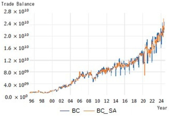
Figure 1.
Trade balance between Mexico and the United States from 1995 to 2024, original and seasonally adjusted series. Source: Prepared by the authors using E-views with data from [10].
Table 1 summarizes the main statistics for both series, facilitating their comparison in terms of central tendency, extremes, and dispersion.

Table 1.
Descriptive statistics for the original and seasonally adjusted trade balance between Mexico and the U.S.
3.1. Trade Balance Analysis Using HP
Figure 2 presents the seasonally adjusted trade balance series (BC_SA) along with its decomposition using the HP filter. The blue line shows the original series, with sustained growth and bouts of volatility, especially in recent years. The green line represents the trend estimated by HP, which smooths out short-term variations and reflects structural developments. The orange line shows the cyclical component, highlighting temporary deviations from the trend, useful for identifying periods of trade expansion and contraction.
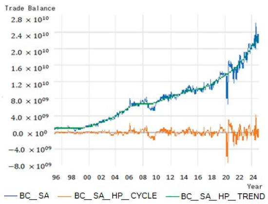
Figure 2.
Seasonally adjusted trade balance between Mexico and the U.S. from January 1995 to November 2024 (value in USD). Source: Prepared by the authors using E-views with data from the Bank of Mexico [10].
This decomposition allows for the analysis of long-term dynamics and economic cycles and serves as a benchmark for comparison with the wavelet approach. The results obtained with HP show a sustained trend and cyclical fluctuations that reflect the evolution of foreign trade between Mexico and the U.S., in a context of high trade dependence.
Regarding the long-term trend, sustained growth is observed, reflecting Mexico’s consolidation within the framework of the North American Free Trade Agreement (NAFTA) (1994–2020) and its transition to the United States–Mexico–Canada Agreement (USMCA) (2020 to date). This upward trend confirms three aspects.
First, there is a sustained increase in bilateral trade, with Mexico consolidating its position as a key player in global value chains, particularly in the automotive, manufacturing, and technology sectors. Second, the structural impact of trade liberalization is notable, as liberalization and productive integration with the U.S. have contributed to greater stability in foreign trade, favoring high-value-added manufacturing exports. Finally, resilient growth in the face of crises is evident, as despite adverse events such as the 2008 financial crisis, the 2014 oil price crash, and the 2020 pandemic, the trade balance has maintained a stable trajectory, consolidating its role as a structural component of the Mexican economy.
On the other hand, the analysis of cyclical fluctuations allows us to identify the impact of various economic crises and external events through temporary deviations from the long-term trend. For example, during the 2008–2009 global financial crisis, a marked decline in the cycle was observed, consistent with the contraction of global trade and the U.S. recession. In 2014, the cycle deteriorated due to the fall in oil prices and its impact on Mexican exports. In 2018, the trade war between the U.S. and China generated an increase in the cycle’s volatility, possibly associated with the reconfiguration of global supply chains. Finally, 2020 saw a sharp contraction followed by a rapid recovery, reflecting the disruption caused by the COVID-19 pandemic and the fiscal stimulus implemented in the US.
The results obtained using the HP filter show that Mexico’s trade balance with the U.S. has followed a path of sustained growth, capable of withstanding various economic crises and external shocks. However, cyclical fluctuations reveal a structural vulnerability to global events, highlighting the need to promote greater market diversification to reduce dependence on the U.S., strengthen regional production chains through the USMCA, and establish response mechanisms to mitigate the impact of international recessions on bilateral trade.
This analysis provides a solid basis for comparison with the results from the wavelet approach and for assessing whether frequency-domain analysis offers a more accurate understanding of bilateral trade dynamics. The series were seasonally adjusted in EViews (version 12) using the X-12 ARIMA method with default parameters. Trend and cycle estimation were performed using the @hpfilter function in the same software, using a smoothing parameter λ = 14,400, suitable for monthly series. These procedures are detailed to ensure the transparency and reproducibility of the analysis, in accordance with good practices in time series studies.
3.2. Analysis of the Trade Balance Using Wavelets
After applying the HP filter and interpreting its results, wavelet analysis was performed as an alternative method. To do this, Python was run on the Google Colab platform using the PyWavelets (pywt) library, using the wavedec() function to perform the orthonormal Discrete Wavelet Transform (DWT). The decomposition was performed using the Daubechies wavelet of order 4 (db4), widely used in economic series due to its convenient temporal localization and smoothness.
A level 4 decomposition was applied, appropriate for the monthly frequency and length of the series. The components—A4 (trend), D1 to D3 (short- and medium-term fluctuations), and D4 (noise)—were reconstructed with the upcoef() function, using the take=len(series) argument to preserve the original length. This technique allows the signal to be analyzed at multiple time scales, offering a more precise view of its fluctuations and noise component. Figure 3 shows this decomposition applied to the trade balance between Mexico and the U.S.
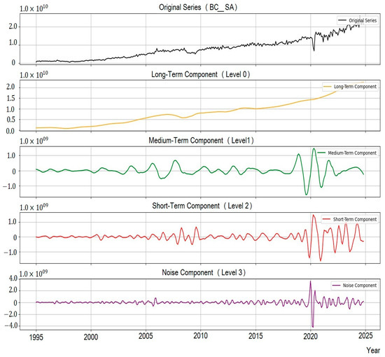
Figure 3.
Multiscale decomposition of the trade balance using wavelets. Source: Prepared by the authors using Python.
The original series (BC_SA) shows the historical evolution of the seasonally adjusted trade balance. The long-term fluctuations (orange line) below reflect structural trends in foreign trade, similar to those estimated with the HP filter. However, unlike the HP filter, which applies smoothing using a penalty parameter, wavelets allow for more precise detection of structural changes associated with trade agreements or tariff policies.
The green line represents medium-term fluctuations associated with business cycles influenced by global demand, monetary policies, or changes in the terms of trade. These cycles may reflect phases of growth or contraction in strategic sectors, such as the manufacturing industry, which is closely linked to trade with the U.S.
The red line represents short-term fluctuations, highlighting high-frequency variations that could be explained by shorter-duration external shocks, such as exchange rate fluctuations, commodity price changes, or production adjustments due to global uncertainty. At this level, wavelets offer a significant advantage over HP, as they allow for a more precise decomposition and analysis of the influence of short-term events, such as financial crises or supply chain disruptions.
The noise component, represented in purple, reflects the residual volatility of the trade balance, attributable to unsystematic factors such as logistical delays, irregular shipments, or political uncertainty. Unlike the HP filter, which imposes a fixed cyclical component, wavelet analysis more accurately captures the stochastic nature of these movements, offering a more realistic representation of high-frequency disturbances. Furthermore, the power spectrum was estimated to observe the variation of the dominant frequencies over time.
Figure 4 presents the wavelet power spectrum applied to the seasonally adjusted trade balance series (SC_SA). This graph displays when and with what intensity fluctuations occur on different time scales, thus providing a dynamic view of the series’ cyclical structure.
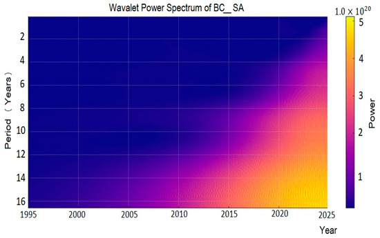
Figure 4.
Wavelet power spectrum of BC_SA. Source: Prepared by the authors using Python.
The horizontal axis represents time (years), while the vertical axis shows the fluctuation period, expressed in years. The colors indicate the strength of each component at each moment in time; the brightest areas (in yellow or red tones) reflect a higher concentration of energy in a cycle of a given duration, while the darker areas represent low activity in that range.
It is also observed that most of the power is concentrated on timescales longer than 8 years, indicating the presence of dominant long-term cycles in the series. In contrast, short periods (less than 3 years) show very little activity, suggesting a limited relevance of high-frequency fluctuations. This representation reinforces the argument in favor of wavelet analysis, as it reveals temporal structures that are not detectable by traditional methods such as the Hodrick–Prescott filter, which assume a rigid separation between cycle and trend.
3.3. The Contrast Between Both Methodologies
The comparison between the HP filter and the DWT is based on both theoretical and practical reasons for analyzing economic series. The HP filter, traditionally used to separate trends and cycles, assumes a constant smoothness that facilitates general macroeconomic analysis. However, this rigidity can underestimate transient shocks and high-frequency fluctuations, limiting its ability to capture short-term events or abrupt changes in the series.
The Wavelet Transform, for its part, allows for a multiscale decomposition of the series, segmenting fluctuations into different time horizons. Theoretically, it offers a more flexible and detailed representation, capable of revealing hidden patterns, identifying structural changes, and more accurately capturing the response of the trade balance to temporary events such as financial crises or trade reforms.
To evaluate the performance of both approaches, three comparison levels were established. First, long-term trends were contrasted: those estimated with the HP filter versus wavelet level 0, which represents the underlying structure of the series. Second, cyclical fluctuations were analyzed over different time horizons, comparing the cycle obtained with the HP filter with wavelet levels 1 to 3, which, together with level 0, make up the four levels analyzed. Finally, we examined which method most accurately captures transient events and structural changes, such as those resulting from NAFTA, the USMCA, and various global economic crises.
From a methodological perspective, the wavelet-reconstructed signal offers a more flexible representation of the trend, allowing for a clearer distinction between short-, medium-, and long-term fluctuations. Compared with the HP filter, wavelets more accurately capture the effects of short-term events and structural changes, providing a more detailed view of the evolution of bilateral trade between Mexico and the U.S.
This analysis seeks to determine whether wavelets offer a more detailed and adaptable view than the HP filter, which would represent a significant methodological advance in the study of the trade balance and other key economic series. To this end, graphs and metrics were used to compare both methods, highlighting the dynamics each captures and the distinct contributions of wavelet analysis compared to the traditional approach.
Figure 5 compares the trend in the trade balance between Mexico and the U.S. estimated using the HP filter and wavelet filters. While both methodologies capture the overall evolution of the series, they present important differences in their behavior.
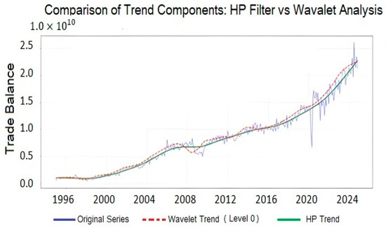
Figure 5.
Comparison of the HP trend with wavelet analysis. Source: Prepared by the authors using Python.
The trend estimated with the HP filter provides a smoother view of the trade balance by eliminating short-term fluctuations. In contrast, the wavelet estimation shows greater sensitivity to changes in the series, adapting better to abrupt variations and short-term events. This capability suggests that wavelet analysis is a more flexible and accurate tool for assessing the evolution of bilateral trade, capturing both long-term trends and adjustments resulting from economic shocks.
On the other hand, Figure 6 compares the cyclical fluctuations in the trade balance obtained using the HP filter and wavelet analysis.
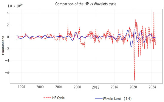
Figure 6.
Comparison of HP cyclical fluctuations with wavelet analysis. Source: Prepared by the authors using Python.
The cycle estimated with the HP filter (red line) exhibits more abrupt variations and greater volatility, while the cycle obtained with wavelets (blue line) smooths these movements and reflects fluctuations across different time horizons with greater stability. This difference is relevant, as the HP filter tends to amplify short-term fluctuations, which can lead to more volatile interpretations of the business cycle. In contrast, wavelet analysis allows the series to be broken down by frequency levels, providing a more nuanced representation of business cycles between Mexico and the U.S., making it a more robust tool, especially in contexts of high uncertainty.
To quantitatively assess these differences, two dimensions were analyzed: the long-term trend and the cyclical components. Regarding the structural trend, both methods produced highly consistent results; the correlation between the two estimates was 0.998, and their fit with respect to the original series was 0.988 for HP and 0.986 for wavelets. These values indicate that both methodologies offer similar estimates of the overall trajectory of the trade balance.
However, when comparing the cyclic components, the differences become significant. The correlation between the cycle estimated by HP and that obtained using wavelets was only −0.091, indicating that each method captures different fluctuation patterns. Furthermore, the Mean Square Error (MSE) was and the Mean Absolute Error (MAE) reached , demonstrating a considerable divergence in the amplitude and direction of the captured oscillations.
These differences are summarized in the following comparison table (Table 2), which presents the main correlation and error metrics for the trends and cycles generated by both approaches.

Table 2.
Statistical comparison between the trends and cycles obtained by the HP filter and wavelet analysis.
Based on the visual results, quantitative metrics, and economic interpretation, wavelets emerge as a more robust and flexible methodology for capturing short-term dynamics, while the HP filter remains useful for analyzing long-term trends.
On the other hand, considering that one of the main limitations of the HP filter is its sensitivity to the smoothing parameter λ, a comparison exercise was carried out to illustrate this dependence. Figure 7 shows the estimated trend on the seasonally adjusted series using two different values of the parameter: the conventional value for monthly data (λ = 14,400) and a high value (λ = 100,000), which imposes a greater degree of smoothness.
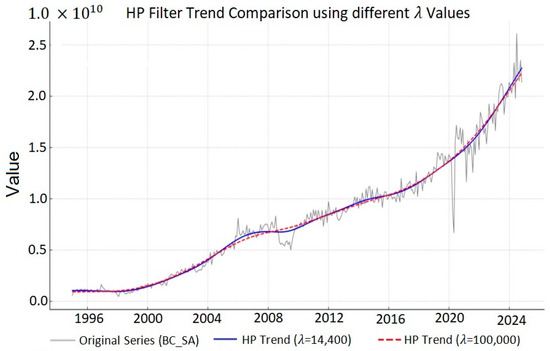
Figure 7.
HP filter trend comparison using different λ values. Source: Prepared by the authors using Python.
Although both curves present a similar general trajectory, differences are observed in the local slope and inflection point detection. These discrepancies are reflected in the MCE between the two estimates, which amounts to 2.59 × 10¹⁶, confirming that parameter selection has a significant impact on the results obtained.
This quantitative evidence supports one of the central arguments of this study—wavelet analysis offers a methodologically more flexible and robust alternative, as it does not rely on a single arbitrary parameter, and is especially useful in contexts where local changes or non-permanent structural fluctuations need to be captured.
4. Conclusions
The analysis of the trade balance between Mexico and the U.S. using wavelet transforms represents a novel methodological contribution to applied economic research. Unlike the HP filter, which imposes a rigid separation between trend and cycle, the wavelet approach allows the series to be decomposed into multiple time scales, more accurately capturing short-, medium-, and long-term fluctuations.
This flexibility is particularly valuable when studying a strategic variable such as the trade balance, whose behavior is influenced by dynamics of varying frequency, such as seasonality, specific economic crises, and structural transformations in trade flows. The use of wavelets in this context not only improves the ability to detect relevant patterns but also represents a methodological innovation applicable to other key economic series.
The results show that the wavelet approach offers a more detailed and realistic representation of trade dynamics by reducing data noise and aligning its fluctuations with historical events such as China’s entry into the World Trade Organization (WTO) in 2001, the 2008 financial crisis, and the COVID-19 pandemic. This reinforces its usefulness as a tool for economic policy analysis and for studying complex phenomena in international trade.
Although the HP filter remains a recognized tool in the economic literature, this study demonstrates that wavelets can complement—or even replace—it in contexts requiring greater sensitivity to short-term variations. In short, the application of wavelets to the analysis of the bilateral trade balance provides a richer and more adaptable perspective, constituting a significant contribution in both methodological and empirical terms, with the potential to be replicated in other foreign trade studies.
Author Contributions
Conceptualization, J.G.C. and X.L.; methodology, J.G.C. and X.L.; software, J.G.C.; validation, J.G.C. and X.L.; formal analysis, X.L.; investigation, J.G.C.; resources, J.G.C. and X.L.; data curation, J.G.C.; writing—original draft preparation, J.G.C.; writing—review and editing, X.L.; visualization, J.G.C.; supervision, X.L.; project administration, X.L.; funding acquisition, J.G.C. All authors have read and agreed to the published version of the manuscript.
Funding
This research was funded by the Programa de Becas Posdoctorales por México of the Secretaría de Ciencia, Humanidades, Tecnología e Innovación (SCHTI), grant number [CVU 417717].
Institutional Review Board Statement
Not applicable.
Informed Consent Statement
Not applicable.
Data Availability Statement
The data used in this study were obtained from the Foreign Trade Cube (Cubo de Comercio Exterior) of Banco de México, which is publicly available at https://www.banxico.org.mx/CuboComercioExterior/ (accessed on 6 February 2025).
Conflicts of Interest
The authors declare that they have no conflicts of interest.
Abbreviations
The following abbreviations are used in this manuscript:
| HP | Hodrick–Prescott (filter) |
| DWT | Discrete Wavelet Transform |
| ARIMA | Autoregressive Integrated Moving Average |
| NAFTA | North American Free Trade Agreement |
| USMCA | United States–Mexico–Canada Agreement |
| MAE | Mean Absolute Error |
| MSE | Mean Squared Error |
| WTO | World Trade Organization |
References
- Singh, R.; Das, D.; Jana, R.K.; Tiwari, A.K. A wavelet analysis for exploring the relationship between economic policy uncertainty and tourist footfalls in the USA. Curr. Issues Tour. 2019, 22, 1789–1796. [Google Scholar] [CrossRef]
- González-Concepción, G.; Gil-Fariña, M.C.; Pestano-Gabino, C.B. Identifying Economic Cycles in Spain Using Wavelet Functions: Oil Price, Industrial Production and Consumer Price Indices. Rev. Iber. Comun. Trab. ASEPUMA 2018, 19, 1–16. [Google Scholar] [CrossRef]
- Hamilton, J.D. Time Series Analysis; Princeton University Press: Princeton, NJ, USA, 1994. [Google Scholar]
- Ravn, M.O.; Uhlig, H. On Adjusting the Hodrick–Prescott Filter for the Frequency of Observations. Rev. Econ. Stat. 2002, 84, 371–376. [Google Scholar] [CrossRef]
- Gençay, R.; Selçuk, F.; Whitcher, B. An Introduction to Wavelets and Other Filtering Methods in Finance and Economics; Academic Press: San Diego, CA, USA, 2001. [Google Scholar] [CrossRef]
- Hodrick, R.J.; Prescott, E.C. Postwar U.S. Business Cycles: An Empirical Investigation. J. Money Credit Bank. 1997, 29, 1–16. [Google Scholar] [CrossRef]
- Hamilton, J.D. Why You Should Never Use the Hodrick–Prescott Filter. Rev. Econ. Stat. 2018, 100, 831–843. [Google Scholar] [CrossRef]
- Crowley, P.M. A Guide to Wavelets for Economists. J. Econ. Surv. 2007, 21, 207–267. [Google Scholar] [CrossRef]
- Findley, D.F.; Monsell, B.C.; Bell, W.R.; Otto, M.C.; Chen, B. New Capabilities and Methods of the X-12-ARIMA Seasonal-Adjustment Program. J. Bus. Econ. Stat. 1998, 16, 127–152. [Google Scholar] [CrossRef]
- Banco de México. Cubo de Comercio Exterior. Available online: https://www.banxico.org.mx/CuboComercioExterior/ (accessed on 6 February 2025).
Disclaimer/Publisher’s Note: The statements, opinions and data contained in all publications are solely those of the individual author(s) and contributor(s) and not of MDPI and/or the editor(s). MDPI and/or the editor(s) disclaim responsibility for any injury to people or property resulting from any ideas, methods, instructions or products referred to in the content. |
© 2025 by the authors. Licensee MDPI, Basel, Switzerland. This article is an open access article distributed under the terms and conditions of the Creative Commons Attribution (CC BY) license (https://creativecommons.org/licenses/by/4.0/).