A Tool for a Fast and Accurate Evaluation of the Energy Production of Bifacial Photovoltaic Modules

Abstract

In this work, we propose a simulation tool designed for the analysis and optimization of bifacial photovoltaic (PV) modules, which are currently under the spotlight in the renewable energy scenario. The tool is conceived to support researchers and engineers by providing fast and accurate predictions of the PV module yield under various operating and environmental conditions. For a chosen geographical site, the impact of module orientation, tilt, albedo, sky conditions, ambient temperature, and so on can be effortlessly determined. In case of nonuniformity across the cells dictated by localized architectural shading, dirt, bird drops, and defects, a circuit-based cell-level approach can be activated to compute the module production. An extensive simulation campaign is performed by assuming that the panels are installed in Naples without loss of generality. Results are shown to give detailed insights into the performance of bifacial modules, thus providing unambiguous guidelines for their correct installation. Further analyses are conducted to demonstrate the tool capability to quantify the detrimental influence of a poorly-irradiated cell on the backside, as well as of cracked cells.

1. Introduction

The global energy landscape is rapidly shifting towards renewable energy sources to alleviate climate change and reduce the dependence on fossil fuels. Among renewable sources, photovoltaic (PV) technology stands out due to its scalability, decreasing costs, and widespread adoption.

Traditionally, the market has been dominated by monofacial PV modules (hereinafter also referred to as panels), which capture sunlight only on one side (front). However, in recent times, bifacial PV modules, engineered to capture sunlight also on the backside (henceforth denoted as rear), have emerged as a valuable alternative, as they are supposed to offer higher energy yields at a price of a minor and affordable upgrade of the fabrication equipment. Promising results have been obtained in many applications like agrivoltaics, aquavoltaics, or in high-reflection environments such as deserts, snow-covered areas, and urban architectures with reflective surfaces (e.g., [1,2,3,4,5,6,7,8,9,10,11] and references therein).

The literature is populated by papers comparing monofacial and bifacial panels in terms of cost, efficiency, and production under various operating conditions [12,13,14,15,16,17,18,19]. However, there is still a lack of unambiguous guidelines defining in which circumstances (in terms of orientation, inclination, reflection from ground, partial shading on either the front or rear and so on) bifacial modules offer clear and distinct advantages with respect to the monofacial counterparts. This challenge can only be addressed by resorting to advanced simulation tools suited to predict the performance of bifacial and monofacial modules in any environment, thereby supporting engineers and researchers in making choices oriented to energy yield and return-on-investment maximization.

In this paper, we present a comprehensive modeling framework, programmatically implemented as a simulation tool, conceived to analyze bifacial PV modules and small-scale plants without overlooking any key details. The proposed tool allows for a fast, yet accurate enough, evaluation of the multifaceted behavior and energy performance of the modules, with total immunity to convergence problems. The required inputs include the day of the year, the geographical coordinates of the installation site, the evolution along the day of total and diffuse irradiance on the horizontal plane, as well as ambient temperature (available on online databases), orientation, tilt, albedo, and some datasheet parameters. The tool determines the current–voltage ($I-V$) characteristic of the module, and thus the maximum produced power, at each clock time in the day. The computation is automated and very fast, taking only tens of seconds to cover a whole day with a 15 min discretization.

The tool is entirely developed as a Matlab code, except when there are discrepancies among the cells in terms of irradiances (on the front and/or on the rear) or other parameters. In such a nonuniform case, Matlab is still used to determine front/rear irradiances and temperature on the cells behaving uniformly, but the circuit simulation program OrCAD PSPICE [20] is invoked to compute the $I-V$ characteristics along the day with a high-granularity cell-level approach. By virtue of this dual-software feature, it is possible to predict the impact of partial architectural shading, bird drops, accumulated dirt, snow, and cell defects (e.g., cracks).

The remainder of this work is articulated as follows: Section 2 details the modeling strategy, offering a clear and comprehensive overview of the adopted formulations. The tutorial-style presentation is designed to inspire readers and provide them with the necessary guidance to confidently and easily implement the methodology themselves. In Section 3, the tool is adopted to explore the daily, monthly, and yearly energy production of bifacial PV modules located in Naples by varying orientation, tilt, and albedo values. The bifacial performance is compared against a south-oriented monofacial module tilted by 30°, which is the optimal condition in Naples and is therefore taken as a reference. It is found that west- or east-oriented vertical bifacial modules outperform the reference monofacial counterpart in terms of yearly energy yield, which makes them suitable for applications like agrivoltaics or noise barriers along highways. Moreover, a counter-intuitive result is achieved: it is shown that the reduction of the current photogenerated by a rear cell (e.g., due to a mud spot) can lead to bypass activation even if the Sun rays are only hitting the front. The detrimental impact of cracked cells is also quantified. Section 3 concludes by highlighting the strengths of the tool over specialized software, namely, easy customization, capability to perform extensive simulation campaigns in a short time, inclusion of an accurate, physically meaningful model for the albedo reflection, and the possibility to execute simulations with cell-level granularity. Conclusions are finally drawn in Section 4.

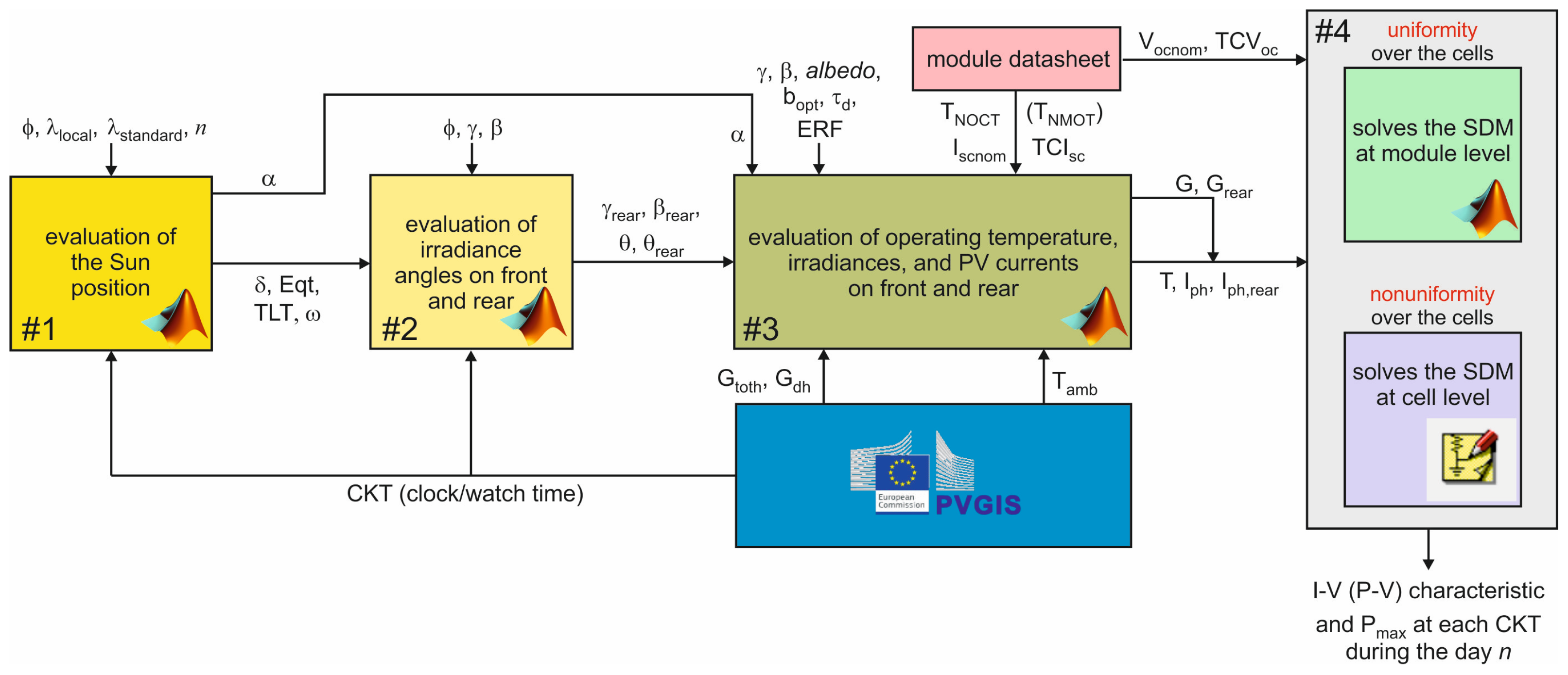
2. The Tool

The block diagram of the tool is represented in Figure 1. As can be seen, the tool is articulated into four primary blocks. Blocks #1, #2, and #3 are Matlab codes, while for #4 two options are possible: (1) if all the cells in the module share the same irradiance on the front, the same irradiance on the rear, as well as the same parameters, a Matlab block is used to solve the single-diode model (SDM) described in Section 2.4 at module level, that is, the voltage drop across the module is obtained by multiplying the voltage drop across the cell $V_{cell}$ by the number of cells embedded in the panel; (2) if there is a nonuniformity among the cells in the module (either on the front or on the rear) in terms of irradiances (dictated by partial shading) and/or electrical parameters (induced by defects), then the solution is handled by the circuit simulator PSPICE, in which each cell is individually described by its own subcircuit. PSPICE was chosen since it is equipped with a robust engine suited for the solution of systems of nonlinear algebraic equations, which ensures short CPU times and unlikely occurrence of convergence problems.

The detailed description of each block is provided in the following.

2.1. Block #1

Block #1 is fed with

• The latitude ϕ and the local longitude $\lambda$, denoted as ${\lambda }_{local}$, of the geographical site where the PV module is installed (ϕ is equal to 0° at the equator and ranges from 0° to 90° to the north and from 0° to −90° to the south; ${\lambda }_{local}$ is equal to 0° at the Prime, or Greenwich, meridian, and ranges from 0° to 180° to the east and from 0° to −180° to the west).
• The longitude ${\lambda }_{standard}$ of the standard meridian on which the clock time (CKT, also referred to as watch time or standard local time) is based.
• The day of the year n.
• The CKT values during the day, i.e., the daytime discretization.

• and calculates

• The solar declination δ, i.e., the angle between the Sun rays (the beam radiation) and the equatorial plane, which is positively defined in the northern hemisphere. Angle δ can be reasonably assumed constant during a day (it varies by at most 0.5°) and is dependent on the day of the year n through the empirical Cooper’s relation

  $$\mathsf{\delta }=23.45\sin \left[{\displaystyle \frac{360}{365}}\left(284+n\right)\right]$$

  (1)

  On the summer solstice, δ assumes the maximum value of 23.45° (23°27′); on the winter solstice, it is equal to the minimum value of −23.45° (−23°–27′); δ = 0° on the spring and autumn equinoxes. It must be observed that (1) assumes a year of exactly 365 days, that is, it does not account for the extra 0.2422 days. Over a span of four years, this approximation would result in a deviation of about one day. One way to modify (1) is to adjust the constant 360/365 to 360/365.24 in the sine argument; however, this adjustment is not strictly necessary, as the error introduced is negligible.
• The so-called True Local Time (TLT), which can be obtained from the CKT by applying two corrections. The first correction is dictated by the difference between the local longitude ${\lambda }_{local}$ and the longitude of the standard meridian ${\lambda }_{standard}$; more specifically, the displacement of 1° between these longitudes corresponds to 4 min. The second correction is made to account for the non-constancy of the rotation rate of the Earth around the Sun during the year. This effect can be described by introducing a characteristic time referred to as Equation of Time (Eqt), expressed in minutes, which depends on n through the following relation [21,22,23]:

  $$Eqt=K_1\left(K_2+K_3\cos B-K_4\sin B-K_5\cos 2B-K_6\sin 2B\right)\hspace{0.17em}\hspace{0.17em}\hspace{0.17em}\hspace{0.17em}\hspace{0.17em}\hspace{0.17em}\hspace{0.17em}\hspace{0.17em}B=\left(n-1\right){\displaystyle \frac{360}{365}}$$

  (2)

  with K₁ = 229.2 min, K₂ = 0.000075, K₃ = 0.001868, K₄ = 0.032077, K₅ = 0.014615, and K₆ = 0.04089 [22,23] (or 0.040849 [21] without appreciable Eqt variation). By applying both corrections, under standard time (standard conditions) the relation between TLT (in hours) and CKT is given by

  $$TLT=CKT-{\displaystyle \frac{4}{60}}\left({\lambda }_{standard}-{\lambda }_{local}\right)+{\displaystyle \frac{Eqt}{60}}$$

  (3)

  which, under daylight-saving time/conditions, is modified into

  $$TLT=CKT-1-{\displaystyle \frac{4}{60}}\left({\mathsf{\lambda }}_{standard}-{\mathsf{\lambda }}_{local}\right)+{\displaystyle \frac{Eqt}{60}}$$

  (4)

  that is, a further hour must be deducted.
• The hour angle ω, i.e., the angular displacement of the Sun with respect to the local meridian compared to the case in which TLT = 12 due to the rotation from west to east of the Earth around its axis (also denoted as angle subtended by the Sun [24]). Angle ω is negative in the morning, positive in the afternoon, and given by [21,23,25,26,27,28]

  $$\mathsf{\omega }=15\left(TLT-12\right)$$

  (5)

  As can be seen, a one-hour deviation corresponds to a displacement of 15°.
• The solar altitude, or elevation, α, i.e., the angle between the horizontal plane (also denoted as plane of horizon) and the Sun rays, positive during daytime; α is a function of latitude ϕ, solar declination δ, and hour angle ω according to [21,24,25,26,27]

  $$\sin \mathsf{\alpha }=\sin \mathsf{\varphi }\sin \mathsf{\delta }+\cos \mathsf{\varphi }\cos \mathsf{\delta }\cos \mathsf{\omega }$$

  (6)

  The outcomes of block #1 for some application examples are reported in

  Table 1. Outputs of block #1 for selected geographical sites, days of the year, and clock times.

  Naples Italy	Stuttgart Germany [21]	Madison WI, USA [22]	Cape Town South Africa
  inputs ϕ = 40°50′ λlocal = 14°15′ λstandard = 15° July 15 (n = 196), CKT = 16 (4:00 PM) daylight-saving time	inputs ϕ = 48°46′ λlocal = 9°10′ λstandard = 15° July 1 (n = 182), CKT = 12 (12:00 AM) daylight-saving time	inputs ϕ = 43°04′ λlocal = −89°–23′ λstandard = −90° February 3 (n = 34), CKT = 10.5 (10:30 AM) standard time	inputs ϕ = −33°–55′ λlocal = 18°25′ λstandard = 30° December 10 (n = 344), CKT = 9.25 (9:15 AM) standard time
  outputs δ = 21.52° Eqt = −5.79 min TLT = 14.85 (2:51 PM) ω = 42.80° α = 49.13°	outputs δ = 23.12° Eqt = −3.46 min TLT = 10.55 (10:33 AM) ω = −21.70° α = 59.15°	outputs δ = −16.97° Eqt = −13.49 min TLT = 10.32 (10:19 AM) ω = −25.26° α = 25.64°	outputs δ = −23.05° Eqt = 7.14 min TLT = 8.60 (8:36 AM) ω = −51.05° α = 44.31°

  .

2.2. Block #2

Block #2 is fed with

• The latitude ϕ of the site.
• The CKT values.
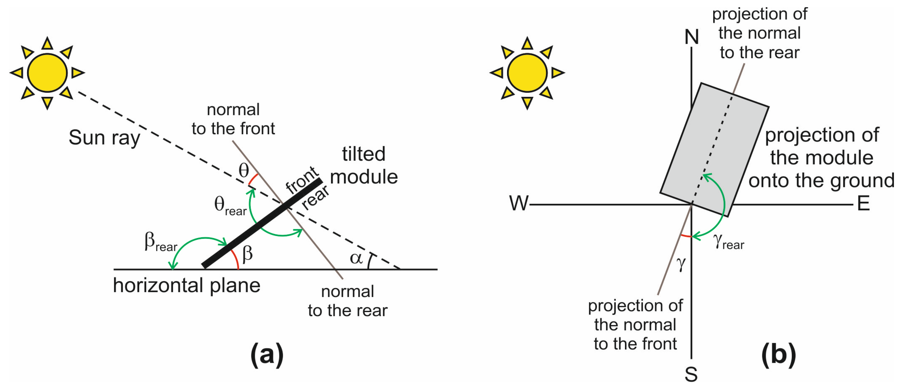
• The azimuth angle of the module front γ, which defines the module orientation, as it is the angular displacement from the south of the projection of the normal to the module front onto the horizontal plane. An azimuth γ = 0° means that the front is south-oriented; γ is positive clockwise (to west), reaching 180° next to north, and is negative counter-clockwise (to east), reaching −180° next to north [22]. Hence, γ = 90° corresponds to a module with a west-oriented front, while γ = −90° identifies an east-oriented front.
• The tilt angle of the module front β, which is the inclination with respect to the horizontal plane.
• The solar declination δ and the hour angle ω computed by block #1.

• and calculates

• The azimuth angle of the module rear ${\mathsf{\gamma }}_{rear}=\mathsf{\gamma }-180°$.
• The tilt angle of the module rear as the supplement of β, that is, ${\mathsf{\beta }}_{rear}=180°-\mathsf{\beta }$.
• The incidence angles of the Sun rays on the module front $\mathsf{\theta }$ and rear ${\mathsf{\theta }}_{rear}$ (both being ≥ 0°). $\mathsf{\theta }$ is the angle between the Sun rays and the normal to the module front, and is evaluated from [21,22,23,24,28]

  $$\begin{array}{c}\cos \mathsf{\theta }=\cos \mathsf{\delta }\cos \mathsf{\omega }\left(\sin \mathsf{\varphi }\cos \mathsf{\gamma }\sin \mathsf{\beta }+\cos \mathsf{\varphi }\cos \mathsf{\beta }\right)+\\ \hspace{1em}\hspace{1em}\hspace{1em}+\sin \mathsf{\delta }\left(\sin \mathsf{\varphi }\cos \mathsf{\beta }-\cos \mathsf{\varphi }\cos \mathsf{\gamma }\sin \mathsf{\beta }\right)+\\ \hspace{1em}\hspace{1em}\hspace{1em}+\cos \mathsf{\delta }\sin \mathsf{\omega }\sin \mathsf{\gamma }\sin \mathsf{\beta }\end{array}$$

  (7)

• It can be inferred that θ = 0° for a horizontal module (β = 0°) at the equator (ϕ = 0°) at TLT = 12 (noon, ω = 0°) of the equinoxes (δ = 0°); angle θ may exceed 90°, which means that the Sun is behind the surface.
• As an example, if it is required to determine the angle of incidence of the Sun rays on the front of a module installed at Madison, WI, USA, with orientation γ = 15° and tilt β = 45° at CKT = 10.7 (10:42 AM) on February 13 (n = 44), then block #1 evaluates that δ = −13.95°, Eqt = −14.26 min, TLT = 10.50 (10:30 AM), ω = −22.50°, α = 29.38°, and block #2 calculates θ = 35° [22].
• ${\mathsf{\theta }}_{rear}$ is the angle between the Sun rays and the normal to the module back, and is computed as $180°-\mathsf{\theta }$ or equivalently from

  $$\begin{array}{c}\cos {\mathsf{\theta }}_{rear}=\cos \mathsf{\delta }\cos \mathsf{\omega }\left(\sin \mathsf{\varphi }\cos {\mathsf{\gamma }}_{rear}\sin {\mathsf{\beta }}_{rear}+\cos \mathsf{\varphi }\cos {\mathsf{\beta }}_{rear}\right)+\\ \hspace{1em}\hspace{1em}\hspace{1em}\hspace{1em}+\sin \mathsf{\delta }\left(\sin \mathsf{\varphi }\cos {\mathsf{\beta }}_{rear}-\cos \mathsf{\varphi }\cos {\mathsf{\gamma }}_{rear}\sin {\mathsf{\beta }}_{rear}\right)+\\ \hspace{1em}\hspace{1em}\hspace{1em}\hspace{1em}+\cos \mathsf{\delta }\sin \mathsf{\omega }\sin {\mathsf{\gamma }}_{rear}\sin {\mathsf{\beta }}_{rear}\end{array}$$

  (8)
• Figure 2 is intended to provide a clear understanding of some key angles introduced so far.

2.3. Block #3

Block #3 relies on the widely-used 2-D representation, i.e., it assumes infinitely-long modules (which corresponds to the practical case of a long row). Its inputs are

• The solar altitude α evaluated by block #1.
• The azimuth angles $\mathsf{\gamma }$, ${\mathsf{\gamma }}_{rear}$, the tilt angles $\mathsf{\beta }$, ${\mathsf{\beta }}_{rear}$, and the incidence angles θ, ${\mathsf{\theta }}_{rear}$.
• The total irradiance $G_{toth}$, the diffuse irradiance $G_{dh}$ hitting the horizontal plane (the beam, or direct, irradiance $G_{bh}$ is determined as $G_{toth}-G_{dh}$), and the ambient temperature $T_{amb}$ vs. CKT at the selected geographical site. For the analysis performed in Section 3, these data were taken from the PhotoVoltaic Geographical Information System (PVGIS) website [29]. Here, it is stated that they were evaluated for the mean day of the chosen month from satellite data through a sophisticated algorithm accounting for sky obstruction (shading) by local terrain features (hills or mountains) calculated from a digital elevation model.
• The albedo value, namely, the ratio of the reflected upward radiation from the ground to the incident downward radiation upon it (typical albedo values are 0.04 for fresh asphalt, 0.1–0.15 for soil ground, 0.25–0.3 for green grass, 0.4 for desert sand, 0.55 for fresh concrete, and 0.8–0.85 for freshly fallen snow).
• Some key parameters available in the datasheet, i.e., the temperature $T_{NOCT}$ (or $T_{NMOT}$), the short-circuit current $I_{scnom}$, and the percentage temperature coefficient $TC{I}_{sc}$ of the short-circuit current $I_{sc}$, the definitions of which will be provided in the following.

• The block calculates

• The beam irradiance impinging on the module front as [21,22,23,24,30,31,32,33]

  $$G_b=\max \left\{0,\hspace{0.17em}\hspace{0.17em}{G}_{bh}{\displaystyle \frac{\cos \mathsf{\theta }}{\sin \mathsf{\alpha }}}\right\}$$

  (9)

  If $\mathsf{\theta }>90°$, the Sun is behind the panel, $\cos \mathsf{\theta }$ becomes negative, and thus $G_b=0\hspace{0.33em}{\mathrm{W}/\mathrm{m}}^2$ from (9).
• The diffuse irradiance on the front coming from the sky, for which there are two options.

• If the sky is completely and densely overcast, the same irradiance comes from any point of the sky, which is thus called isotropic. In this case, the diffuse irradiance is expressed as

  $$G_{di}=G_{dh}{F}_i$$

  (10)

  where the dimensionless front-sky view factor $F_i$ (≤1) accounts for the reduction of the sky dome due to the tilt angle β; using the cross-string approach [34], it can be easily determined that

  $$F_i={\displaystyle \frac{1+\cos \mathsf{\beta }}{2}}={\cos }^2{\displaystyle \frac{\mathsf{\beta }}{2}}$$

  (11)

  Formulation (11), sometimes referred to as Kondrat’yev’s view factor [35], is widely accepted [2,9,10,12,13,21,22,23,24,25,26,30,31,36,37,38,39,40,41,42,43,44], and coincides with the ratio between the projection onto the horizontal plane of the portion of the hemisphere seen from the tilted panel and the projection of the whole sky dome [45].
• If the sky is clear or at least partially cloudy, the diffuse irradiance depends on the position of the Sun in the sky due to effects like horizon brightening and circumsolar radiation, and the sky is thus referred to as anisotropic. In this case, the diffuse irradiance can be expressed as

  $$G_{da}=G_{dh}{F}_a$$

  (12)

  where the front-sky view factor $F_a$ is given by the sum of two terms $F_{a1}$ and $F_{a2}$ accounting for the horizon brightening and circumsolar radiation, respectively [22,31,33].

  $$F_a=F_{a1}+F_{a2}=F_i\left(1-A_i\right)\left(1+f{\sin }^3{\displaystyle \frac{\mathsf{\beta }}{2}}\right)+\max \left\{0,\hspace{0.33em}{A}_i{\displaystyle \frac{\cos \mathsf{\theta }}{\sin \mathsf{\alpha }}}\right\}$$

  (13)

  In (13),

  $$f=\sqrt{{\displaystyle \frac{G_{bh}}{G_{toth}}}}$$

  (14)

  and $A_i$ is the anisotropic index, given by

  $$A_i={\displaystyle \frac{G_{bh}}{G_0}}$$

  (15)

  where $G_0$ is the solar irradiance incident on a horizontal plane outside the atmosphere, also referred to as extraterrestrial irradiance on a horizontal surface, whose expression is [22,33]

  $$G_0=G_{sc}\left[1+0.033\cos \left({\displaystyle \frac{360}{365}}n\right)\right]\left(\cos \mathsf{\varphi }\cos \mathsf{\delta }\cos \mathsf{\omega }+\sin \mathsf{\varphi }\sin \mathsf{\delta }\right)$$

  (16)

  $G_{sc}=1353\hspace{0.17em}{\mathrm{W}/\mathrm{m}}^2$ being the solar constant.

• Differently from the isotropic view factor $F_i$, the anisotropic one $F_a$ can be >1 if the panel is oriented to the portion of the sky dome where the Sun is located. It is worth noting that $F_a$ reduces to $F_i$ if $G_{bh}=0\hspace{0.33em}{\mathrm{W}/\mathrm{m}}^2$ (uniformly cloudy, or isotropic, sky), which implies that $f=0$ and $A_i=0$.

• The diffuse irradiance on the front due to the reflection from the ground, typically considered as a Lambertian (isotropic) process, calculated as

  $$G_{d,albedo}=G_{toth}\cdot albedo\cdot F_{albedo}$$

  (17)

  where the front-ground view factor $F_{albedo}$ is expressed as [2,9,10,12,13,21,22,23,30,31,32,33,36,37,38,39,40,42,44,46,47]

  $$F_{albedo}={\displaystyle \frac{1-\cos \mathsf{\beta }}{2}}={\sin }^2{\displaystyle \frac{\mathsf{\beta }}{2}}$$

  (18)

  Model (18) works quite well in the entire range of practical β values, namely, from β = 0° (horizontal panel) to β = 90° (vertically-deployed panel); $F_{albedo}=0$ if β = 0° since the panel front does not see the ground (it only sees the sky); $F_{albedo}$ increases with β and becomes eventually equal to 0.5 if β = 90° since the front sees half ground.

• It is worth noting that under isotropic conditions the sum of the front-sky and front-ground view factors is 1, that is,

  $$F_i+F_{albedo}=1$$

  (19)

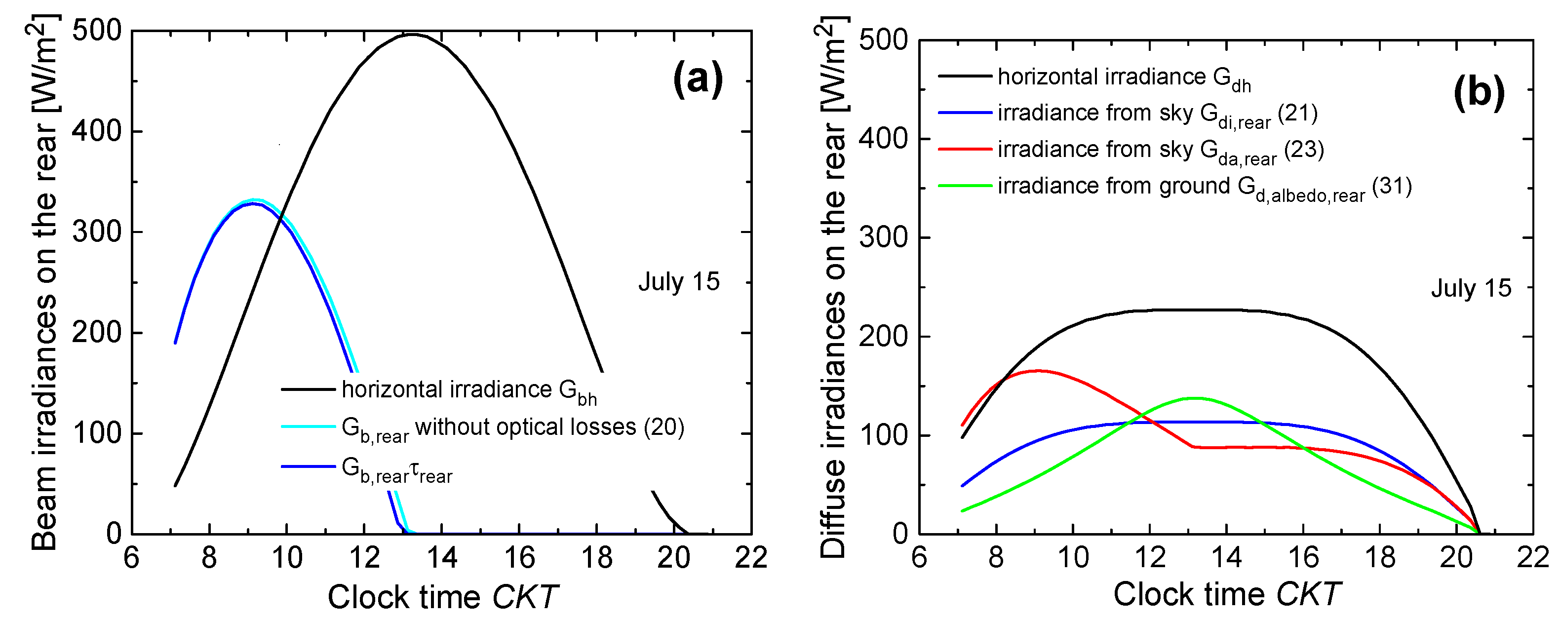
• The beam irradiance landing on the rear

  $$G_{b,rear}=\max \left\{0,\hspace{0.33em}{G}_{bh}{\displaystyle \frac{\cos {\mathsf{\theta }}_{rear}}{\sin \mathsf{\alpha }}}\right\}=\max \left\{0,\hspace{0.33em}-G_{bh}{\displaystyle \frac{\cos \mathsf{\theta }}{\sin \mathsf{\alpha }}}\right\}$$

  (20)
• The diffuse irradiance on the rear coming from the sky. Analogously to the module front, there are two possible options.

• Under isotropic conditions, the diffuse irradiance is given by

  $$G_{di,rear}=G_{dh}{F}_{i,rear}$$

  (21)

  with the rear-sky view factor [2,42,44]

  $$F_{i,rear}={\displaystyle \frac{1+\cos {\mathsf{\beta }}_{rear}}{2}}={\cos }^2{\displaystyle \frac{{\mathsf{\beta }}_{rear}}{2}}={\displaystyle \frac{1-\cos \mathsf{\beta }}{2}}={\sin }^2{\displaystyle \frac{\mathsf{\beta }}{2}}$$

  (22)

  Under anisotropic conditions,

  $$G_{da,rear}=G_{dh}{F}_{a,rear}$$

  (23)

  where

  $$F_{a,rear}=F_{a1,rear}+F_{a2,rear}=F_{i,rear}\left(1-A_i\right)\left(1+f{\sin }^3{\displaystyle \frac{{\mathsf{\beta }}_{rear}}{2}}\right)+\max \left\{0,\hspace{0.33em}{A}_i{\displaystyle \frac{\cos {\mathsf{\theta }}_{rear}}{\sin \mathsf{\alpha }}}\right\}$$

  (24)

• The diffuse irradiance on the rear due to the reflection from the ground, which deserves significant attention, as discussed in our recent work [48]. One might mistakenly apply the same approach used for the frontside and express this irradiance as

  $$G_{d,albedo,rear}=G_{toth}\cdot albedo\cdot F_{albedo,rear}$$

  (25)

  with the rear-ground view factor $F_{albedo,rear}$ given by [41,42,43,44]

  $$F_{albedo,rear}={\displaystyle \frac{1-\cos {\mathsf{\beta }}_{rear}}{2}}={\sin }^2{\displaystyle \frac{{\mathsf{\beta }}_{rear}}{2}}={\displaystyle \frac{1+\cos \mathsf{\beta }}{2}}={\cos }^2{\displaystyle \frac{\mathsf{\beta }}{2}}$$

  (26)

• Unfortunately, different from (17), model (25) does not provide physically meaningful results within the range of practical β values. If β is reduced from 90° to 0°, $F_{albedo,rear}$ increases, eventually becoming 1 for β = 0° (horizontal panel with the frontside oriented towards the sky and backside lying on the ground); as a result, $G_{d,albedo,rear}$ incorrectly increases as β decreases and reaches its maximum value for β = 0° when instead it should be 0 W/m², as the ground beneath the flat panel cannot reflect sunlight. This is the consequence of the incorrectness of (25), which assumes that the ground reflects an irradiance given by $G_{toth}\cdot albedo$ independently of the inclination of the module and thus of the sky dome visible to the ground. In addition, (25) does not consider the shadow cast by the module itself onto the ground (self-shading) and does not include the dependence upon the vertical distance d between the module edge and the ground. The standard strategy to account for the self-shading is to express $G_{d,albedo,rear}$ as [6,9,13,42,47,49]

  $$G_{d,albedo,rear}=G_{toth}\cdot albedo\cdot F_{albedo,rear,unshaded}+G_{dh}\cdot albedo\cdot F_{albedo,rear,shaded}$$

  (27)

  where $F_{albedo,rear,unshaded}$ is the view factor between rear and unshaded ground, whereas $F_{albedo,rear,shaded}$ is the view factor between rear and ground shaded by the panel. For the case d = 0 (lowest panel edge in contact with the ground), such view factors can be determined by resorting to the cross-string rule and are given by [42,48]

  $$F_{albedo,rear,unshaded}={\displaystyle \frac{\sin \mathsf{\beta }}{2}}\cdot {\displaystyle \frac{1-\cos \mathsf{\alpha }}{\sin \mathsf{\alpha }}}$$

  (28)

  $$F_{albedo,rear,shaded}={\displaystyle \frac{1+\cos \mathsf{\beta }}{2}}-{\displaystyle \frac{\sin \mathsf{\beta }}{2}}\cdot {\displaystyle \frac{1-\cos \mathsf{\alpha }}{\sin \mathsf{\alpha }}}$$

  (29)
• It is worth noting that

  $$F_{i,rear}+F_{albedo,rear,unshaded}+F_{albedo,rear,shaded}=1$$

  (30)

  However, also (27) provides unreasonable results since $G_{dh}\cdot albedo\cdot F_{albedo,rear,shaded}$ incorrectly increases with decreasing β and tends to its maximum value for β = 0°, when it is expected to be 0 W/m² since the backside lies flat on the ground.
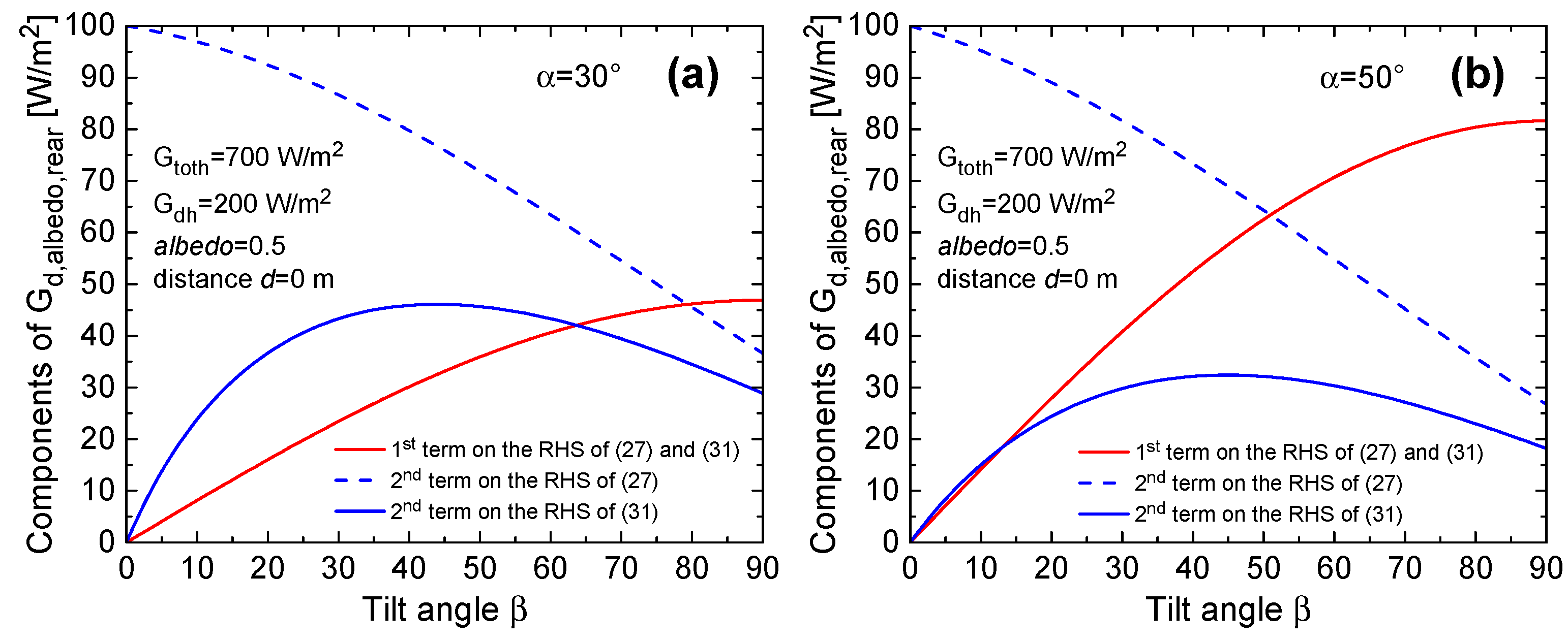
• In [48], we proposed an improved version of (27) to solve this inconsistency, namely,

  $$G_{d,albedo,rear}=G_{toth}\cdot albedo\cdot F_{albedo,rear,unshaded}+G_{dh}\cdot F_{shaded-sky}\cdot albedo\cdot F_{albedo,rear,shaded}$$

  (31)

  where $F_{shaded-sky}$ is the view factor between shaded ground and sky, and is given by

  $$F_{shaded-sky}={\displaystyle \frac{\cos \mathsf{\beta }+\sin \mathsf{\beta }\cdot \frac{1+\cos \mathsf{\alpha }}{\sin \mathsf{\alpha }}-1}{2\left(\cos \mathsf{\beta }+\frac{\sin \mathsf{\beta }}{\tan \mathsf{\alpha }}\right)}}$$

  (32)

  Our modeling methodology includes formulation (31) with (28), (29), and (32) for $F_{albedo,rear,unshaded}$, $F_{albedo,rear,shaded}$, and $F_{shaded-sky}$, as well as extended variants for these view factors to capture the case of panels mounted on a suspended framework (d > 0 m) [48]. Figure 3 clearly demonstrates the physical validity of our approach. More specifically, such a figure shows the behavior of the 1st and 2nd terms on the right-hand side (RHS) of (31), namely, $G_{toth}\cdot albedo\cdot F_{albedo,rear,unshaded}$ and $G_{dh}\cdot F_{shaded-sky}\cdot albedo\cdot F_{albedo,rear,shaded}$ by varying β for $G_{toth}=700\hspace{0.33em}{\mathrm{W}/\mathrm{m}}^2$, $G_{dh}=200\hspace{0.33em}{\mathrm{W}/\mathrm{m}}^2$, albedo = 0.5, d = 0 m, with α = 30° (Figure 3a) and α = 50° (Figure 3b). It can be inferred that, if β = 0°, both contributions are equal to 0 W/m², as the backside entirely lies on the ground, so that $F_{albedo,rear,unshaded}=0$ and, despite $F_{albedo,rear,shaded}=1$, the 2nd term $G_{dh}\cdot F_{shaded-sky}\cdot albedo\cdot F_{albedo,rear,shaded}$ is equal to 0 since the shaded area of the ground does not see the sky ($F_{shaded-sky}=0$). Also shown in Figure 3 is the meaningless behavior that would be obtained by using the 2nd term $G_{dh}\cdot albedo\cdot F_{albedo,rear,shaded}$ on the RHS of (27). Further details can be found in [48].

Figure 3. 1st (solid red line) and 2nd (solid blue) terms on the right-hand side (RHS) of (31), along with the 2nd term on the RHS of (27) (dashed blue) as a function of tilt angle β for G_toth = 700 W/m², G_dh = 200 W/m², albedo = 0.5, d = 0 m, (a) α = 30°, (b) α = 50°.

Figure 3. 1st (solid red line) and 2nd (solid blue) terms on the right-hand side (RHS) of (31), along with the 2nd term on the RHS of (27) (dashed blue) as a function of tilt angle β for G_toth = 700 W/m², G_dh = 200 W/m², albedo = 0.5, d = 0 m, (a) α = 30°, (b) α = 50°.

• The reduction in beam irradiance on the front due to optical losses under realistic operating conditions [50] is modeled by multiplying the irradiance (9) by a dimensionless reduction factor dependent on the incidence angle θ and given by

  $$\mathsf{\tau }=1-b_{opt}\left({\displaystyle \frac{1}{\cos \mathsf{\theta }}}-1\right)$$

  (33)

  where $b_{opt}$ is an empirical parameter; τ is forced to be 0 for θ values giving rise to $1-b_{opt}\left({\displaystyle \frac{1}{\cos \mathsf{\theta }}}-1\right)<0$ or $1-b_{opt}\left({\displaystyle \frac{1}{\cos \mathsf{\theta }}}-1\right)>1$. In a similar fashion, the reduction in beam irradiance on the rear is described by multiplying the irradiance (20) by

  $${\mathsf{\tau }}_{rear}=1-b_{opt}\left({\displaystyle \frac{1}{\cos {\mathsf{\theta }}_{rear}}}-1\right)$$

  (34)

  The optical losses affecting the total diffuse irradiance given by the sum of the sky and ground contributions are only negligibly dependent on θ, and thus they are incorporated by multiplying the diffuse irradiance on both front and rear by a constant reduction factor ${\mathsf{\tau }}_d$ (typically in the range of 0.9 to 0.95).

Figure 4 shows the irradiances determined by block#3 on the rear of a west-oriented (γ = 90°) vertically-deployed (β = 90°) bifacial module in Naples (ϕ = 40°50′, ${\lambda }_{local}=14°15\prime$) vs. clock time CKT on July 15. More specifically, Figure 4a illustrates the beam irradiance $G_{b,rear}$ obtained with (20) and the beam irradiance accounting for optical losses computed by multiplying (20) by the reduction factor ${\mathsf{\tau }}_{rear}$ given by (34), along with the horizontal irradiance $G_{bh}=G_{toth}-G_{dh}$, $G_{toth}$ and $G_{dh}$ being sourced from PVGIS. Figure 4b depicts the diffuse irradiance from sky under isotropic conditions $G_{di,rear}$ given by (21), the diffuse irradiance from sky under anisotropic conditions $G_{da,rear}$ given by (23), as well as the irradiance reflected from the ground given by the innovative model (31), along with the horizontal irradiance $G_{dh}$ taken from PVGIS.

• The total irradiances on the front (G) and rear ($G_{rear}$). As first suggested in [30] and commonly accepted since then, the evaluation of the total irradiance hitting the panel is performed by summing the contributions due to the beam irradiance, the diffuse irradiance from the sky, and the diffuse irradiance reflected from the ground (transposition approach).

• Concerning the front,

  $$G=G_b\mathsf{\tau }+\left(G_{di}+G_{d,albedo}\right){\mathsf{\tau }}_d$$

  (35)

  for an isotropic sky, or

  $$G=G_b\mathsf{\tau }+\left(G_{da}+G_{d,albedo}\right){\mathsf{\tau }}_d$$

  (36)

  for an anisotropic one.
• Concerning the rear,

  $$G_{rear}=G_{b,rear}{\mathsf{\tau }}_{rear}+\left(G_{di,rear}+G_{d,albedo,rear}\right){\mathsf{\tau }}_d$$

  (37)

  for an isotropic sky, and

  $$G_{rear}=G_{b,rear}{\mathsf{\tau }}_{rear}+\left(G_{da,rear}+G_{d,albedo,rear}\right){\mathsf{\tau }}_d$$

  (38)

  for an anisotropic one.

• The operating temperature T of the cells as a function of CKT. By disregarding the self-heating, which is a reasonable approximation when the cells are producing power, T [°C] is a function of $T_{amb}$, $G$, and $G_{rear}$ according to the following law [6,9,12,51]:

  $$T=T_{amb}+\left(T_{NOCT}-20°\right){\displaystyle \frac{G+G_{rear}}{G_{nomT}}}$$

  (39)

  where $T_{NOCT}$ is the nominal operating temperature (NOCT) measured on the panel backside under open-circuit conditions at $T_{amb}=20 °\mathrm{C}$, nominal irradiance $G_{nomT}=800\hspace{0.33em}{\mathrm{W}/\mathrm{m}}^2$, air mass AM 1.5, and wind speed lower than 1 m/s. As mentioned earlier, $T_{amb}$ vs. CKT at the selected geographical site is taken from PVGIS, and the total irradiances on the module front (G) and rear ($G_{rear}$) are evaluated by the tool. In (39), it is in principle possible to multiply $G_{rear}$ by an empirical coefficient c (<1) related to the bifaciality factor, i.e., the ratio between the power produced by the rear illuminated under standard test conditions (STCs) while the front is covered, and the power produced by the front illuminated under STCs while the rear is covered; STCs are defined below. Formulation (39) is also referred to as the NOCT model.

• On the other hand, as lucidly expressed in [52], in recent years manufacturers have questioned the uncertainty due to large fluctuations in NOCT and have expressed doubts about the reliability of NOCT-based energy assessments. Consequently, NOCT tests have been replaced by nominal module operating temperature (NMOT) tests; $T_{NMOT}$ represents the temperature measured on the backside while the module is connected to a load, the experimental procedure being reported in [52,53]. For modern bifacial modules, whose datasheets provide $T_{NMOT}$, the tool computes the cell temperature T as

  $$T=T_{NMOT}+\Delta T_{c-b}{\displaystyle \frac{G+G_{rear}}{G_{nomT}}}$$

  (40)

  where $\Delta T_{c-b}$ is the temperature difference between the cell and backside at $G_{nomT}$, usually in the range of 2 to 3 °C. Formulation (40) is denoted as NMOT model.

• Once the irradiance G and the temperature T vs. CKT are known, the current photogenerated by the module front is evaluated at each CKT as [24,54]

  $$I_{ph}=I_{scnom}{\displaystyle \frac{G}{G_{nom}}}+\mathsf{\kappa }\left(T-25°\right)$$

  (41)

  where the datasheet parameter $I_{scnom}$ is the short-circuit current measured by keeping the frontside under STCs, i.e., nominal irradiance $G_{nom}=1000\hspace{0.33em}{\mathrm{W}/\mathrm{m}}^2$, 1.5 AM, and cell temperature equal to 25 °C, and covering the backside or at least markedly limiting its irradiance. It is worth noting that the first term on the RHS is the photogenerated current that would be obtained for an irradiance G at T = 25 °C. The temperature coefficient κ [A/°C] can be easily determined from the datasheet parameter $TC{I}_{sc}$ [%/°C], namely, the percentage temperature coefficient of $I_{sc}$ measured by the module manufacturer under the same conditions mentioned above; $TC{I}_{sc}$ is given by

  $$TC{I}_{sc}={\displaystyle \frac{100}{I_{scnom}}}{\displaystyle \frac{\partial I_{sc}}{\partial T}}={\displaystyle \frac{100}{I_{scnom}}}\mathsf{\kappa }$$

  (42)

• Equation (41) allows capturing the positive temperature coefficient of $I_{ph}$ due to the bandgap shrinking and the resulting increase in the number of photons with enough energy to generate electron–hole pairs, and can be recast as

  $$I_{ph}=I_{scnom}{\displaystyle \frac{G}{G_{nom}}}+\mathsf{\kappa }\left(T-T_0+T_0-25°\right)=I_{scnom}{\displaystyle \frac{G}{G_{nom}}}+\mathsf{\kappa }\left(\Delta T+T_0-25°\right)$$

  (43)

  where $T_0$ is a reference temperature and $\Delta T=T-T_0$; by assuming $T_0=27 °\mathrm{C}$ for consistency with PSPICE [41,55],

  $$I_{ph}=I_{scnom}{\displaystyle \frac{G}{G_{nom}}}+\mathsf{\kappa }\left(\Delta T+2°\right)$$

  (44)
• The current photogenerated by the module rear vs. CKT is calculated as

  $$I_{ph,rear}=ERF\left[I_{scnom}{\displaystyle \frac{G_{rear}}{G_{nom}}}+\mathsf{\kappa }\left(T-25°\right)\right]=ERF\left[I_{scnom}{\displaystyle \frac{G_{rear}}{G_{nom}}}+\mathsf{\kappa }\left(\Delta T+2°\right)\right]$$

  (45)

  where ERF (<1) is an efficiency reduction factor needed to account for the fact that the PV cell is asymmetric, being technologically designed to maximize light absorption on the front, and T is given by (39) or (40).

2.4. Block #4

Block #4 is intended to evaluate the $I-V$ characteristic of the module (and consequently the maximum produced power $P_{max}$) at each CKT during the day.

The individual cell is described through an extended version of the SDM presented in [41,43,55,56] and inspired by [57]. In particular, the cell current $I_{cell}$ is expressed as

$$I_{cell}=I_{ph}+I_{ph,rear}-I_D-I_{sh}+I_{av}$$

(46)

$I_{ph}$ and $I_{ph,rear}$ being given by (44) and (45). In (46), $I_D$ is the current flowing through the intrinsic resistance-free diode. The expression of $I_D$ is derived from the well-known Shockley’s equation

$$I_D\left(T\right)=I_0\left(T\right)\left[\exp \left({\displaystyle \frac{V_D}{\mathsf{\eta }{V}_T}}\right)-1\right]$$

(47)

where $V_D$ is the voltage drop across the diode, given by

$$V_D=V_{cell}+R_s{I}_{cell}$$

(48)

$V_{cell}$ and $R_s$ being the voltage drop over the cell and the series resistance, the dimensionless parameter η is the ideality coefficient, and $V_T={\displaystyle \frac{k}{q}}\left(T+273\right)$ is the thermal voltage, with k and q being the Boltzmann’s constant and the elementary charge. As described in detail in [43,55,58], (47) can be conveniently modified into

$$I_D\left(\Delta T\right)=I_0\left(T_0\right)\left[\exp \left({\displaystyle \frac{V_D+{\mathsf{\varphi }}_0\Delta T}{\mathsf{\eta }{V}_{T0}+\mathsf{\eta }\frac{k}{q}\Delta T}}\right)-1\right]$$

(49)

which better evidences the diode current dependence on the temperature increase $\Delta T=T-T_0$. The value of the key coefficient ϕ₀ is extracted through the following procedure. As illustrated in Figure 1, block #4 also receives the open-circuit voltage $V_{ocnom}$ of the module front and the temperature coefficient $TC{V}_{oc}$ of the open-circuit voltage $V_{oc}$, both measured by keeping the frontside under STCs and the backside covered; $TC{V}_{oc}$ is given by

$$TC{V}_{oc}={\displaystyle \frac{100}{V_{ocnom}}}{\displaystyle \frac{\partial V_{oc}}{\partial T}}$$

(50)

from which ${\displaystyle \frac{\partial V_{oc}}{\partial T}}$ is determined. Then, block #4 executes Matlab simulations of the module with covered backside (setting $I_{ph,rear}=0\hspace{0.33em}\mathrm{A}$) with $G=G_{nom}=1000\hspace{0.33em}{\mathrm{W}/\mathrm{m}}^2$ and T = 25 °C and 30 °C and automatically calculates ${\displaystyle \frac{\partial V_{oc}}{\partial T}}$; parameter ϕ₀ is calibrated to obtain a good agreement between the ${\displaystyle \frac{\partial V_{oc}}{\partial T}}$ value resulting from $I-V$ simulations and the one calculated from (50).

$I_{sh}$ is the current traversing the shunt resistance $R_{sh}$, given by

$$I_{sh}={\displaystyle \frac{V_D}{R_{sh}}}$$

(51)

Resistance $R_{sh}$ is assumed to be temperature-insensitive; nevertheless, $R_{sh}$ might exhibit a negative temperature coefficient induced by the thermal trapping–detrapping of carriers through the defect states in the space charge region [59].

$I_{av}$ is the (positive) avalanche current induced by a reiterated impact-ionization mechanism (avalanche multiplication) in the space-charge region of the cell when subject to high reverse voltages, e.g., in the presence of localized shading; $I_{av}$ is expressed as

$$I_{av}=-{\displaystyle \frac{V_D}{R_{sh}}}{\displaystyle \frac{a_{II}}{{\left(1-\frac{V_D}{BV}\right)}^{m_{II}}}}$$

(52)

where BV (<0 V) is the breakdown voltage of the junction, while $a_{II}$ and $m_{II}$ are dimensionless fitting parameters. From (52), it can be inferred that if $V_D$ is positive, then the denominator of (52) is high and $I_{av}$ is negligible; instead, if $V_D$ is negative and approaches the negative BV, then the positive $I_{av}$ increases and tends to infinity. The temperature-related mitigation of avalanche multiplication can be enabled through the relation

$$BV\left(\Delta T\right)=BV\left(T_0\right)\exp \left(b_{II}\Delta T\right)$$

(53)

$b_{II}$ [°C⁻¹] (>0) being another fitting parameter.

For the series resistance $R_s$, a positive temperature coefficient is accounted for according to the following power relation:

$$R_s\left(\Delta T\right)=R_s\left(T_0\right){\left({\displaystyle \frac{T_0+273+\Delta T}{T_0+273}}\right)}^{m_R}$$

(54)

with $m_R>0$, although in principle any other law (e.g., exponential [60] or linear) can be implemented and enabled.

It was mentioned that if all the cells in the module share the same G, $G_{rear}$, and the same model parameters, the tool resorts to Matlab to solve the SDM given by (46) with (48), (49), (51), (52), (54) at module level: once the $I_{cell}-V_{cell}$ characteristic is evaluated at a selected CKT, the $I-V$ curve of the module is obtained by considering $I=I_{cell}$ and $V=N\cdot I_{cell}$, N being the number of cells in the module.

Instead, if any nonuniformity is present, the commercial circuit simulator OrCAD PSPICE is enabled to compute the $I-V$ characteristic by extending to bifacial modules the approach proposed for monofacial panels in [41,43,55,56,61,62]. PSPICE is a widespread tool well suited to solve systems of algebraic equations in electrical and electronics engineering. Its robust and optimized engine allows preventing large requirements in terms of CPU time and memory storage, as well as potential convergence issues, which would arise by adopting other approaches. Using Simulink [63,64,65] for the simulations in [41,43,56,61] turned out to be a challenging or even unviable solution. Moreover, PSPICE allows for an easy integration of an equivalent compact electrical network (composed of controlled sources, resistors, and capacitors, and denoted as thermal feedback block, or TFB) to efficiently describe the dynamic heat propagation in the module, i.e., the power–temperature feedback, which is required when cells dissipate power. Such an approach was already implemented and used for monofacial panels [41,43] by resorting to a Matlab code referred to as FANTASTIC [66], which receives as an input the 3-D replica of the panel built in the environment of the software COMSOL based on the finite-element method [67] and automatically extracts the TFB. In the proposed tool developed for bifacial modules, we will integrate an advanced TFB accounting for nonlinear thermal effects, as determined by an extended version of FANTASTIC called TONIC [68].

The PSPICE-based strategy can be described as follows:

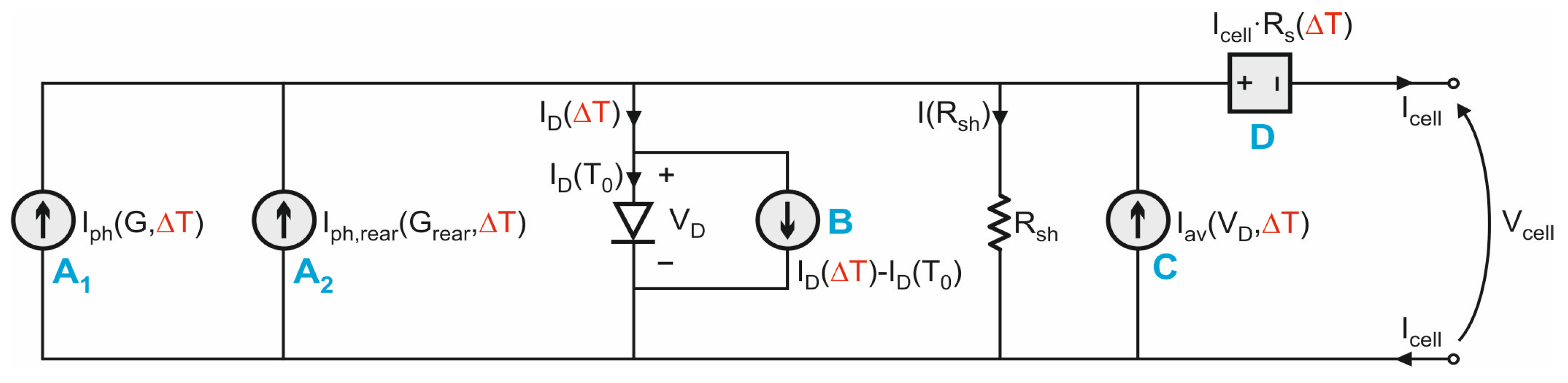
• The module is composed of N series-connected cells, each modeled with a subcircuit implementing the SDM described above, which is fed with G, $G_{rear}$, and $\Delta T=T-T_0$.
• The module can be partitioned into a chosen number of subpanels, each equipped with a bypass diode.
• The PSPICE temperature of all components embedded in the circuit is forced to the reference value $T_0=27\hspace{0.33em}°\mathrm{C}$; the temperature rise $\Delta T$, represented as a voltage, is provided to analog behavioral modeling, or ABM, components, i.e., nonlinear current/voltage sources, to modify the temperature-sensitive parameters (e.g., [69]).

An illustrative sketch of the subcircuit modeling the individual cell is shown in Figure 5.

The ABM components A₁ and A₂ calculate the currents photogenerated by the module front and rear using (44) and (45), respectively. The standard diode, being at the reference temperature $T_0$, conducts the current

$$I_D\left(T_0\right)=I_0\left(T_0\right)\left[\exp \left({\displaystyle \frac{V_D}{\mathsf{\eta }{V}_{T0}}}\right)-1\right]$$

(55)

where $V_{T0}$ is equal to ${\displaystyle \frac{k}{q}}\left(T_0+273\right)$. In order to allow the flow of the temperature-dependent current $I_D\left(\Delta T\right)$ given by (49) in the diode branch, the ABM B is used, which calculates and forces the current $I_D\left(\Delta T\right)-I_D\left(T_0\right)$, $I_D\left(\Delta T\right)$ being evaluated with (49).

To account for the avalanche multiplication, the cell current $I_{cell}$ is computed as the sum of an avalanche-free current (i.e., the current that would flow in the absence of avalanche), and an avalanche-dictated current $I_{av}$ forced by the ABM C and given by (52).

The power dependence on temperature of the series resistance $R_s$ is implemented by forcing on the branch traversed by $I_{cell}$ a voltage drop given by the product between $I_{cell}$ and $R_s$, where $R_s$ is expressed by (54). This is put into practice by making use of the ABM designated as D in Figure 5, which accepts as inputs the temperature rise $\Delta T$ and the current $I_{cell}$ (transformed into a voltage) and imposes the drop $I_{cell}{R}_s\left(\Delta T\right)$.

2.5. Simplified Variant of the Tool for Monofacial Modules

A simplified tool variant is also available, which allows simulating monofacial modules and strings. In this variant:

• Block #1 coincides with the analogous block of the tool for bifacial panels.
• Block #2 only determines the incidence angle θ.
• Block #3 evaluates G, T, $I_{ph}$, where T is given by

  $$T=T_{amb}+\left(T_{NOCT}-20°\right){\displaystyle \frac{G}{G_{nomT}}}$$

  (56)

  according to the NOCT model [27,56,63], or by

  $$T=T_{NMOT}+\Delta T_{c-b}{\displaystyle \frac{G}{G_{nomT}}}$$

  (57)

  according to the NMOT approach.
• Block #4 solves the SDM only with the source for the current $I_{ph}$ photogenerated by the front.

3. Results and Discussion

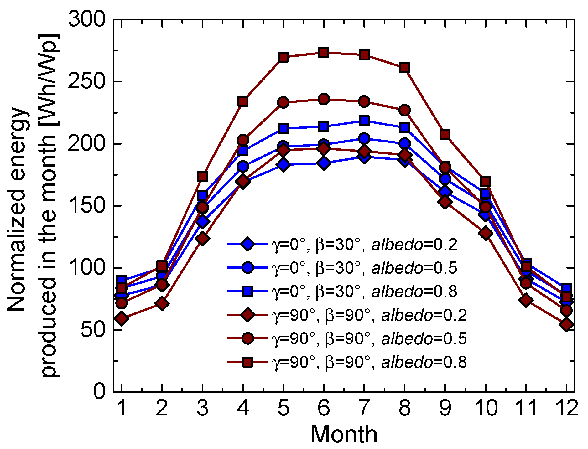
3.1. Optimization of Orientation and Tilt for a Bifacial Module

This section demonstrates the effectiveness of the proposed tool in optimizing the orientation and tilt of a bifacial module at a chosen geographical site.

The site selected as a case-study is again Naples (ϕ = 40°50′, ${\lambda }_{local}=14°15\prime$). It is widely accepted that for the northern hemisphere the yearly energy production for a monofacial panel is maximized if the panel is oriented to the south (γ = 0°) and the tilt angle is determined by the empirical rule of thumb β = ϕ − 15° to ϕ − 10°, which allows for the best performance (the minimum average θ value) from the spring equinox to the autumn one, i.e., when there is the maximum energy availability [22,23,27,39,70], although β deviations up to 15° are expected to marginally affect the energy yield [22]. We performed preliminary simulations of a south-oriented monofacial module showing that the yearly energy production is maximized with β = 30° (=ϕ − 10°), it is negligibly impacted when increasing β up to 45° (=ϕ + 5°), and decreases by 5% when reducing β down to 15% (=ϕ − 25°). Hence, we chose γ and β equal to 0° and 30°, respectively. Such a condition, schematically shown in Figure 6a, will be henceforth considered as a reference to assess the performance of bifacial modules in the same technology.

The analysis was performed by considering the monofacial ET Solar silicon module ET-M54050 embedding N = 40 cells and subdivided into two 20-cell subpanels, each equipped with a bypass diode [41,43,55,56].

The key datasheet parameters are peak power of 50 Wp, $I_{scnom}=2.81\hspace{0.33em}\mathrm{A}$, $T_{NOCT}=44.4\hspace{0.33em}°\mathrm{C}$, $TC{I}_{sc}=0.06\hspace{0.33em}\%/°\mathrm{C}$, and $TC{V}_{oc}=-0.397\hspace{0.33em}\%/°\mathrm{C}$, while the other (either calculated or optimized) model parameters are κ = 1.69 mV/°C, $I_0\left(T_0\right)=8\hspace{0.33em}\mathrm{nA}$, η = 1.2, ϕ₀ = 4.4 mV/°C, $R_{sh}=100\hspace{0.33em}\mathsf{\Omega }$, BV = −15 V, $a_{II}=0.1$, $m_{II}=1.1$, $R_s\left(T_0\right)=12\hspace{0.33em}\mathrm{m}\mathsf{\Omega }$, and $m_R=1.5$. The extension of the cell model to the bifacial case was made by adding in parallel to the current source $I_{ph}$ another current source forcing a photogenerated current $I_{ph,rear}$ given by (45), where ERF was chosen equal to 0.9, that is, the efficiency on the rear was assumed to be 90% of that on the frontside.

The investigation was carried out for d = 0 (i) by initially assuming that the cells share the same irradiances and model parameters, (ii) by considering clear-sky anisotropic conditions from April to October and isotropic sky conditions for the other months, and (iii) setting $b_{opt}=0.05$ and ${\mathsf{\tau }}_d=0.95$ for the optical losses.

Under the above assumptions, the tool was used to evaluate the $I-V$ characteristic of both the monofacial and the corresponding bifacial panel as a function of CKT for a given day of the year n; consequently, the maximum power produced $P_{max}$ was determined at each CKT, and the daily produced energy was calculated by integrating $P_{max}$ over the whole day. The monthly energy was obtained by multiplying the energy produced on a representative day of the selected month (the 15th in our analysis) by the number of days in that month; for instance, the energy produced in April was determined multiplying by 30 the energy produced on April 15. This simplified approach allowed speeding up the analysis without significantly sacrificing the accuracy of the results.

Figure 7 shows the energy production over one year normalized to the peak power (50 Wp) for the reference monofacial module (south-oriented, i.e., with γ = 0°, and tilted by β = 30°) and for the corresponding (γ = 0°, β = 30°) bifacial module for various albedo values. It can be inferred that (i) due to the low tilt angle, the reflection from the ground does not significantly impact the production of the monofacial panel, and (ii) the energy increment obtained with a bifacial module under this condition is marginal due to the poor irradiance contribution of the rear.

In Figure 8, both the monofacial and bifacial panels are south-oriented (γ = 0°) and vertically deployed (β = 90°); the vertical arrangement draws interest as more bifacial modules can be installed in the same field. In this case, using a monofacial module is not convenient since from April to September the angle of incidence is on average rather high, and therefore the energy production is low. Unlike the β = 30° inclination, here using a bifacial panel allows obtaining a significant gain, as the backside is also hit by beam irradiance.

Figure 9a,b report the case of west- (γ = 90°) and east-oriented (γ = −90°) vertical (β = 90°) modules, respectively. Again, the monofacial module is compared with the corresponding bifacial one for different albedo values. The following considerations are in order:

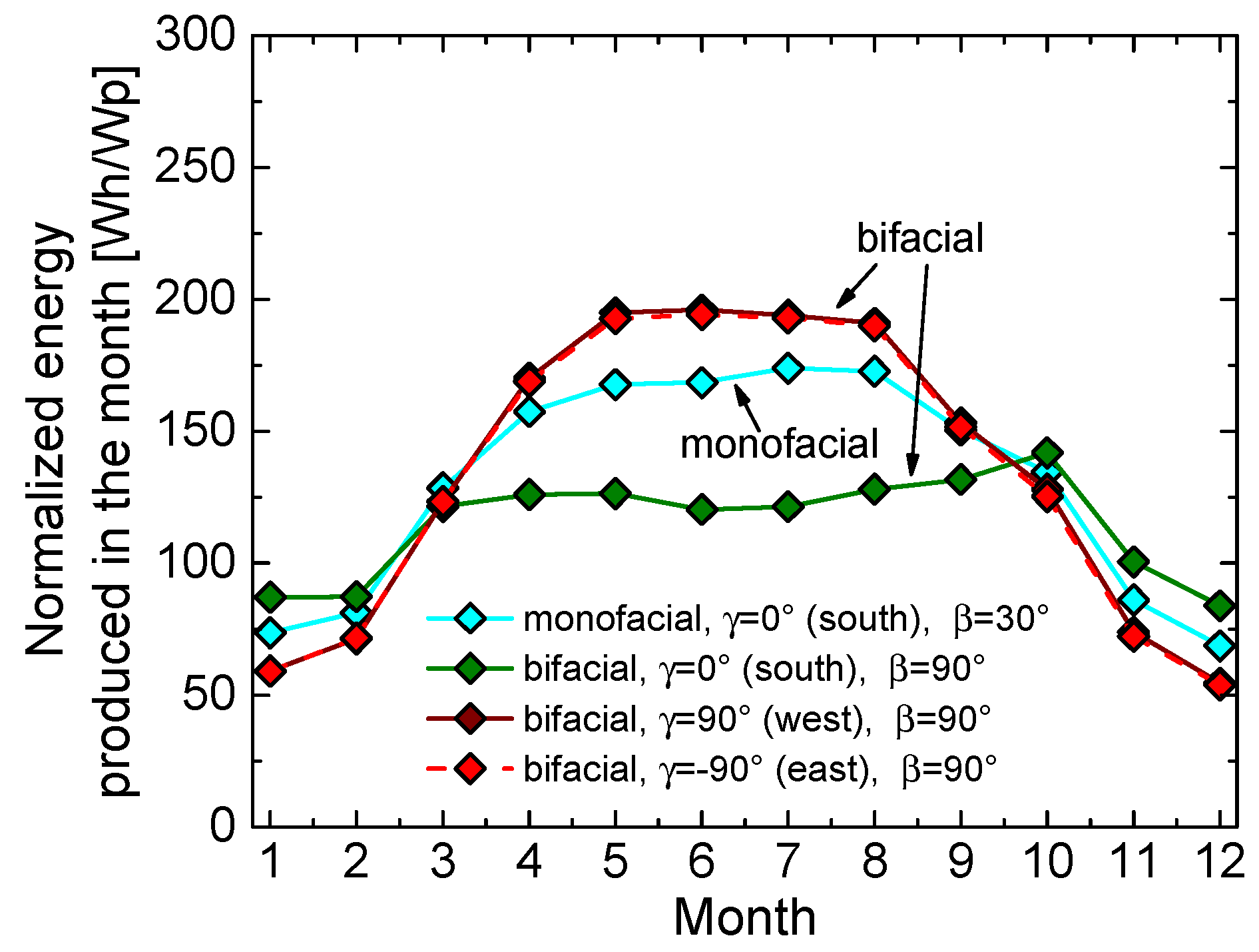
• By specifically referring to the monofacial module, the energy produced by orienting the frontside to the west is slightly better than the one obtained by orienting it to the east; this result is reasonable since Naples faces the sea to the west, while mountains lie to the east.
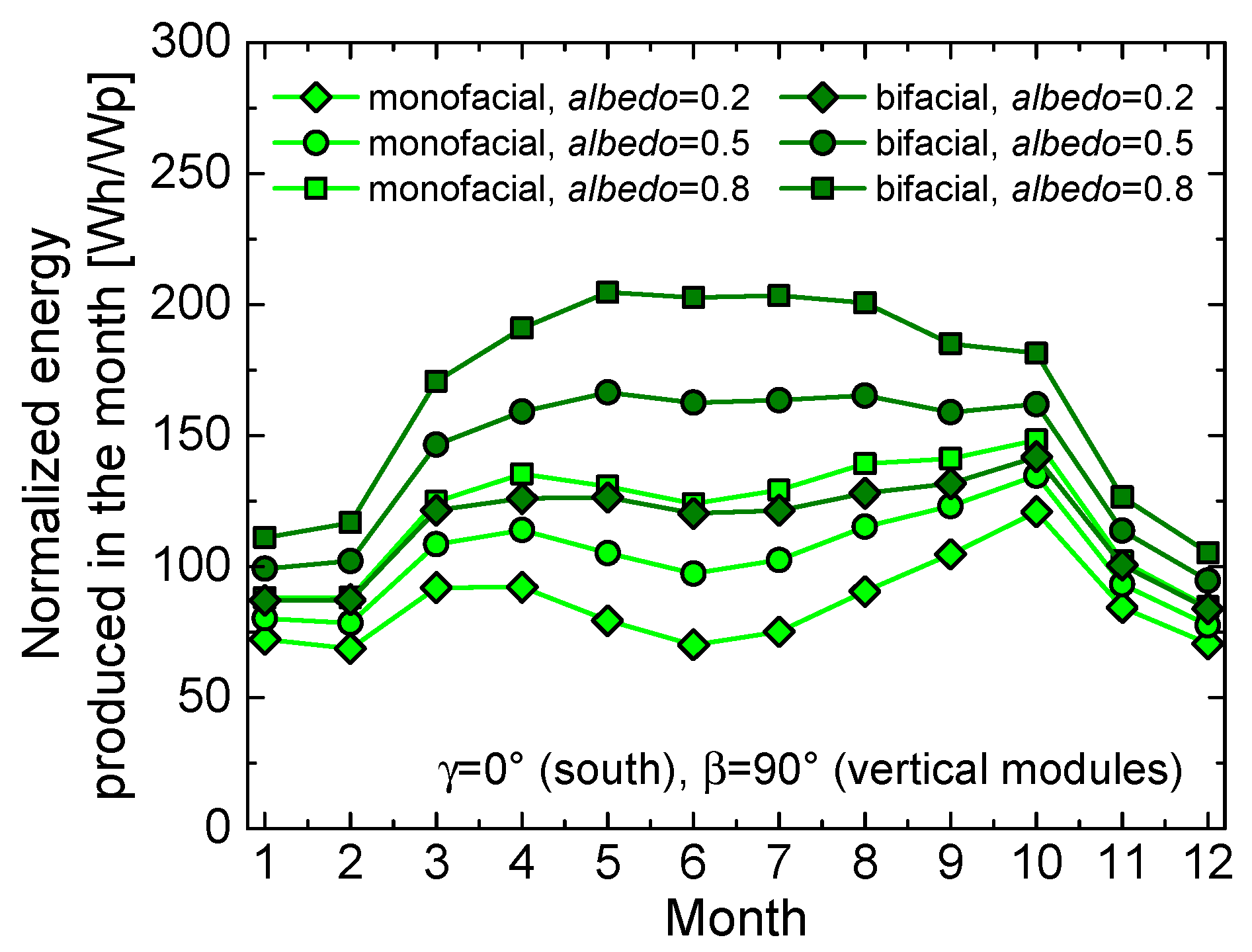
• As a main finding, it is observed that in these cases the bifacial module allows achieving a significant improvement. While the monofacial panel receives beam irradiance for only half of the day, bifacial panels benefit from effective beam irradiance (hitting the module sides with low incidence angles) both in the morning (rear for a west-oriented panel, as sketched in Figure 6b, and front for an east-oriented one) and afternoon (the other way around).
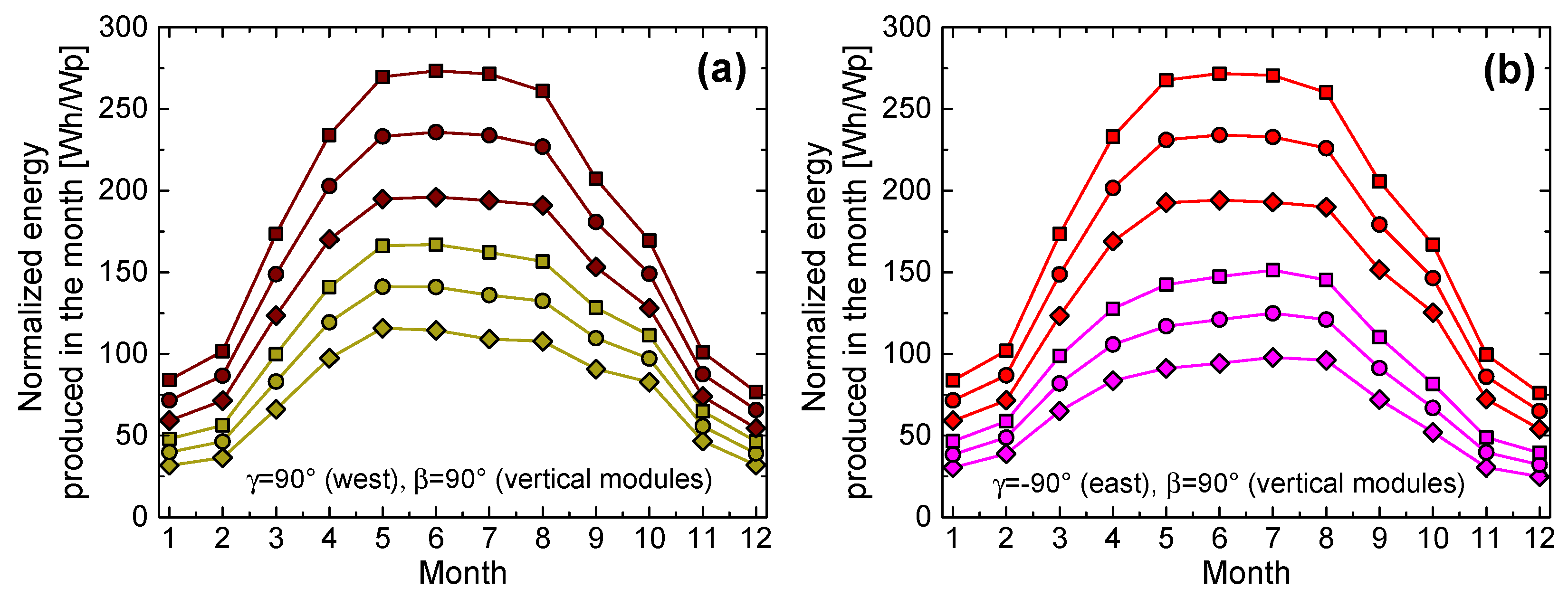
• West- and east-oriented vertical bifacial panels produce the same amount of energy.

In Figure 10, the normalized energies produced by the vertical bifacial panels for a south-, west-, and east-oriented front are compared with the reference monofacial case (the albedo being 0.2 for all cases). By inspecting the curves, it can be inferred that:

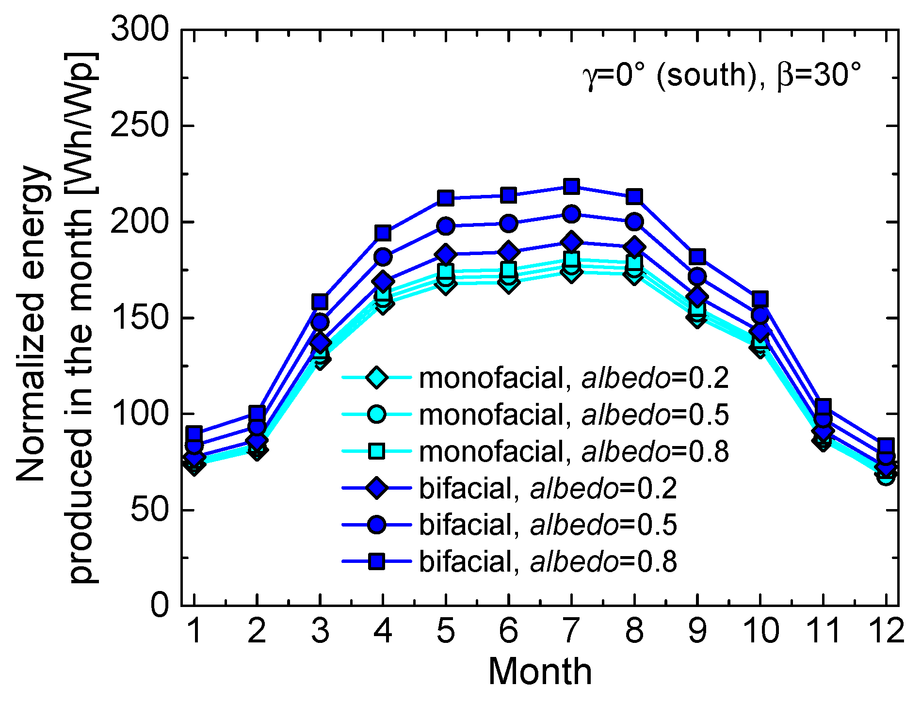
• West- and east-oriented vertical bifacial modules offer improved performance with respect to the reference monofacial counterpart during the time span from April to September, in which they benefit from a low incidence angle of the Sun rays hitting the front and rear of the panel in the mid-morning and mid-afternoon [1,5,10]. In terms of yearly energies (all reported in

  Table 2. Normalized yearly energies for all the cases examined in Section 3.1.

  Orientation (γ) and Tilt (β)	Normalized Yearly-Produced Energy [Wh/Wp]
  	Monofacial	Bifacial
  γ = 0° (south), β = 30°	1560 (albedo = 0.2) reference 1590 (albedo = 0.5) reference 1620 (albedo = 0.8) reference	1680 (albedo = 0.2) 1810 (albedo = 0.5) 1930 (albedo = 0.8)
  γ = 0° (south), β = 90°	1020 (albedo = 0.2) 1230 (albedo = 0.5) 1440 (albedo = 0.8)	1380 (albedo = 0.2) 1690 (albedo = 0.5) 2000 (albedo = 0.8)
  γ = 90° (west), β = 90°	930 (albedo = 0.2) 1140 (albedo = 0.5) 1350 (albedo = 0.8)	1610 (albedo = 0.2) 1920 (albedo = 0.5) 2220 (albedo = 0.8)
  γ = −90° (east), β = 90°	780 (albedo = 0.2) 990 (albedo = 0.5) 1200 (albedo = 0.8)	1600 (albedo = 0.2) 1910 (albedo = 0.5) 2210 (albedo = 0.8)

  ), the gain compared with the reference monofacial case amounts to 3%, 21%, and 37% for albedo values of 0.2, 0.5, and 0.8, respectively.
• West- and east-oriented vertical bifacial modules also provide a considerable production improvement with respect to the south-oriented vertical bifacial counterpart, which is estimated to be 17%, 14%, and 11% for albedo values of 0.2, 0.5, and 0.8, respectively. This is again due to the much better performance of west- and east-oriented panels from April to September, while during wintertime the south-oriented module performs better. An in-depth insight into this behavior can be achieved by showing the normalized maximum power over CKT on July 15 (Figure 11a) and December 15 (Figure 11b) for such cases. In July (and more in general during the whole period from late spring to early autumn), it is confirmed that the orientations of the module front to west and east allow for a very effective exploitation of the beam light impinging on one of the two sides in the mid-morning and on the other in the mid-afternoon, whereas in December (and more in general during wintertime) the orientation to south is better over the mid-day. Throughout the whole year, the first effect markedly prevails over the second.

Figure 10. Normalized energy produced in the months of the year for the reference south-oriented (γ = 0°) monofacial panel tilted by β = 30° (cyan line) and various vertical (β = 90°) bifacial panels, namely, with south-oriented (γ = 0°, dark green), west-oriented (γ = 90°, wine), and east-oriented (γ = −90°, red) front, the latter two practically coinciding, all installed in Naples. An albedo = 0.2 was considered for all cases.

Figure 10. Normalized energy produced in the months of the year for the reference south-oriented (γ = 0°) monofacial panel tilted by β = 30° (cyan line) and various vertical (β = 90°) bifacial panels, namely, with south-oriented (γ = 0°, dark green), west-oriented (γ = 90°, wine), and east-oriented (γ = −90°, red) front, the latter two practically coinciding, all installed in Naples. An albedo = 0.2 was considered for all cases.

Figure 11. Normalized maximum power vs. CKT on (a) July 15 and (b) December 15 for vertical (β = 90°) bifacial modules, with south- (γ = 0°, dark green line), west- (γ = 90°, wine), and east-oriented (γ = −90°, red) front. An albedo = 0.2 was considered for all cases.

Figure 11. Normalized maximum power vs. CKT on (a) July 15 and (b) December 15 for vertical (β = 90°) bifacial modules, with south- (γ = 0°, dark green line), west- (γ = 90°, wine), and east-oriented (γ = −90°, red) front. An albedo = 0.2 was considered for all cases.

Lastly, west- and east-oriented vertical bifacial modules are compared with the south-oriented bifacial one tilted by the optimum β = 30°. From Figure 12 and Table 2, it can be inferred that for albedo = 0.2 the latter performs slightly better, while the vertical ones ensure a superior production for higher albedo values. Such a finding aligns fairly well with that derived in [2], where a simplified analysis only based on the evaluation of annual irradiance [kWh/m²] incident on single (i.e., not included in rows) bifacial PV modules was performed by considering Tel Aviv (ϕ = 32°04′, ${\lambda }_{local}=34°46\prime$) as a geographical site. More specifically, west- (γ = 90°) and east-oriented (γ = −90°) vertical (β = 90°) bifacial modules were compared with a south-oriented (γ = 0°) bifacial one tilted by β = 20°, optimum angle given by the empirical rule ϕ − 15° to ϕ − 10°. It was found that (i) the annual incident irradiance is significantly higher for the latter panel, although its rear side suffers from a negligible irradiance contribution; (ii) vertical bifacial modules can produce more annual energy than a bifacial one with an optimum tilt angle if the ground albedo is very high.

A key conclusion of this analysis is that west- and east-oriented vertical bifacial panels can be recommended for some applications in Naples (and more in general in Italy), e.g., for agrivoltaics, as the vertical installation does not significantly reduce the land available for cultivation, or for building noise barriers along highways, especially for high albedo values.

3.2. Nonuniform Irradiance Distribution over the Panel Rear

Let us consider the scenario of a vertical (β = 90°) bifacial module with an east-oriented front (γ = −90°) located in Naples for agrivoltaics applications (albedo = 0.2, d = 0, ERF = 0.9) on July 15. Under clear-sky conditions, the outcomes of block #3 are as follows:

• G = 412 W/m², $G_{rear}=124\hspace{0.33em}{\mathrm{W}/\mathrm{m}}^2$, T = 43.2 °C, $I_{ph}=1.19\hspace{0.33em}\mathrm{A}$, $I_{ph,rear}=0.34\hspace{0.33em}\mathrm{A}$ at 11:00 AM
• G = 147 W/m², $G_{rear}=391\hspace{0.33em}{\mathrm{W}/\mathrm{m}}^2$, T = 44.1 °C, $I_{ph}=0.44\hspace{0.33em}\mathrm{A}$, $I_{ph,rear}=1.02\hspace{0.33em}\mathrm{A}$ at 3:00 p.m.

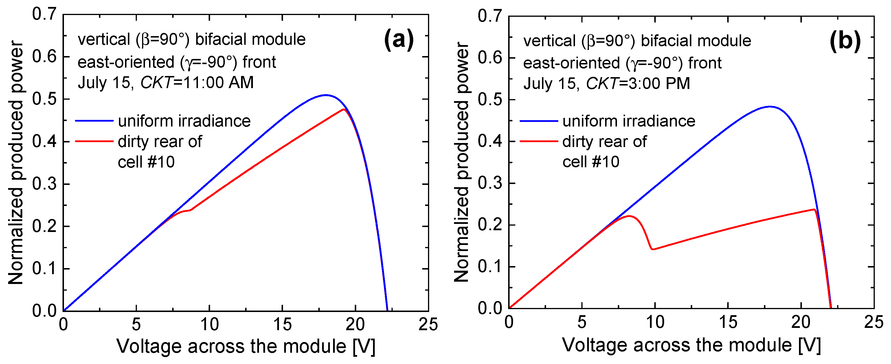
• The normalized power vs. voltage characteristics of the module under uniform irradiance conditions are reported in Figure 13a (CKT = 11:00 AM) and 13b (CKT = 3:00 PM); the maximum powers normalized to the peak value provided in the datasheet are 0.51 and 0.48, respectively. A likely case of a mud spot partially covering the rear of cell #10, sketched in Figure 14, was then considered, which was assumed to reduce the irradiance down to 10% of that of the clean cells. As can be seen, the PSPICE simulations lead to a counter-intuitive result, that is, although the spot is located on the rear, submodule #1 embedding cell #10 is bypassed also in the morning (CKT = 11:00 AM) when the Sun rays hit the module front; such surprising detrimental behavior cannot be overlooked for a more complete comparison between west- or east-oriented vertical bifacial panels and the reference monofacial counterpart. In the afternoon (CKT = 3:00 PM), when the Sun rays impinge on the backside, the power production dramatically drops, as expected.

3.3. Cracked Cell(s)

The proposed tool is also suited to describe a condition with malfunctioning or defective cells. Let us again consider the scenario of a vertical (β = 90°) bifacial module with east-oriented front (γ = −90°) located in Naples for agrivoltaics applications (albedo = 0.2, d = 0 m, ERF = 0.9) on July 15. Under clear-sky conditions, the outputs of block #3 at 10:00 AM are: G = 500 W/m², $G_{rear}=114\hspace{0.33em}{\mathrm{W}/\mathrm{m}}^2$, T = 44.6 °C, $I_{ph}=1.44\hspace{0.33em}\mathrm{A}$, and $I_{ph,rear}=0.32\hspace{0.33em}\mathrm{A}$. Figure 15 illustrates the normalized power against voltage for the panel under normal conditions, i.e., with all non-defective cells. Then the PSPICE-based block #4 was used to assess the impact of cracked cells [71], which were emulated by setting the shunt resistance $R_{sh}$ to 1 Ω instead of 100 Ω. In particular, the cases of one, two, and three cracked cells belonging to submodule #1 were simulated, and the resulting power–voltage curves were reported in Figure 15 as well. 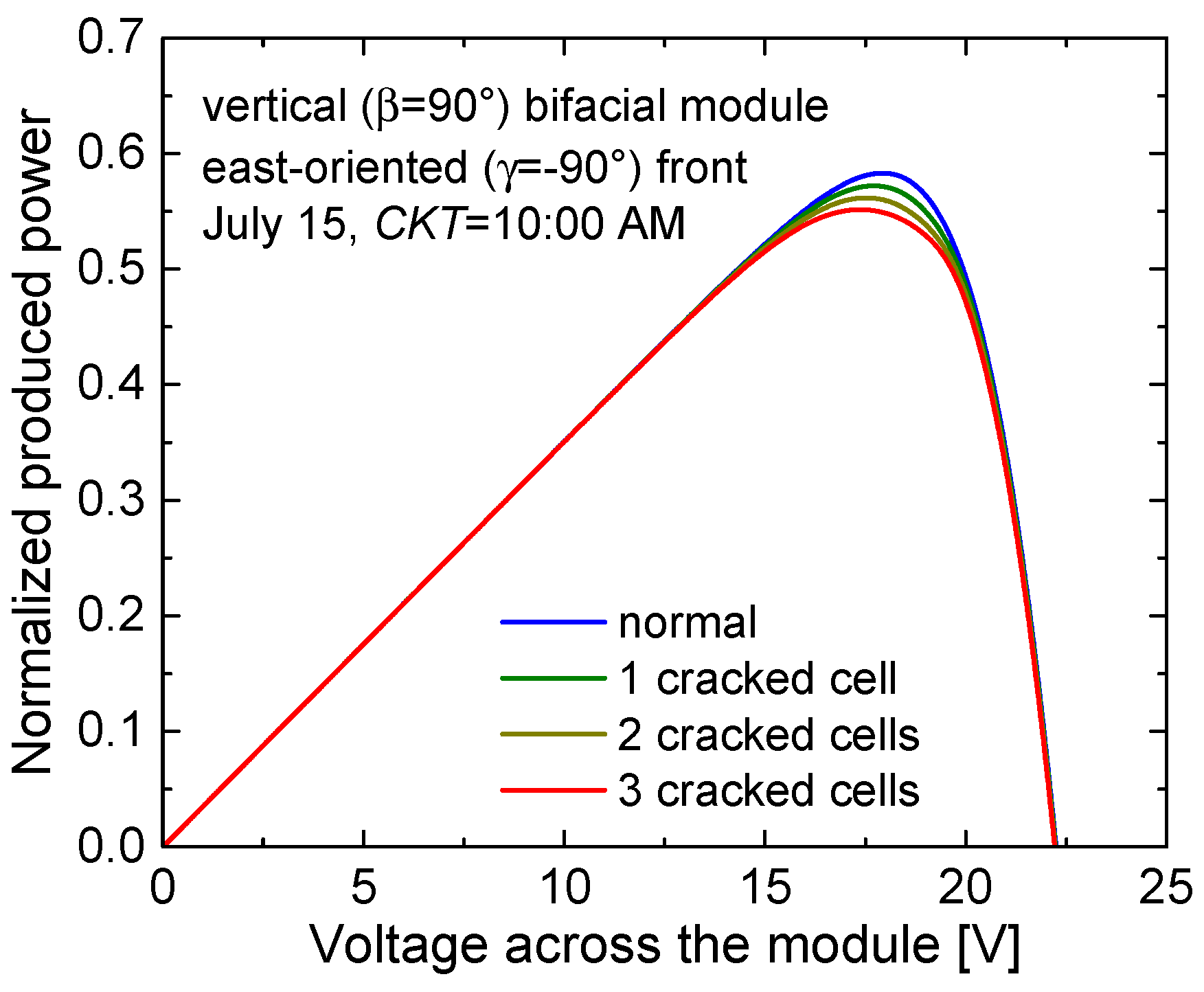It can be observed that the yield degradation is perceptible only for a significant number of damaged cells.

3.4. Summary of the Main Advantages of the Tool and Comparison with Other Programs

The distinctive strengths of our tool can be summarized as follows:

• High flexibility, that is, straightforward customization; it is very easy to modify an analytical model or integrate a new one, to adjust the value of a parameter, and so on.
• Simple monitoring and storing of all the relevant quantities for better insight into the panel behavior and performance.
• Capability of performing extensive simulation campaigns (e.g., parametric studies) in a short time.
• Inclusion of an innovative, physically-meaningful albedo reflection modeling strategy.
• Accurate description of the effects of (even small) architectural or cloud-induced shadows, bird drops, localized accumulation of dirt, dust, snow, other residues, and presence of defective/cracked cells through the PSPICE-based block #4 that benefits from cell-level discretization.
• Possibility of including a thermal feedback block in the PSPICE environment for a high-granularity dynamic electrothermal simulation of the module (already implemented in the tool variant for monofacial panels [41,43]).

It is worth noting that other commercial or open-source software tools are available, which represent an industry/academic standard for design, optimization, and performance forecasting of grid-connected PV systems, besides being capable of providing economic assessment for project feasibility. However, such tools suffer from some limitations, namely, they (i) improperly model the albedo reflection on the backside, (ii) do not generally allow incorporating new models, and (iii) rely on a coarse subpanel- or panel-level discretization; due to the latter issue, they are not suited to fully capture the real behavior of a panel or plant subject to (potentially harmful) small shadows. Based on these observations, although our modeling framework is not intended as a general alternative to other widely-used programs, its implementation and adoption should be recommended for performing fast, yet accurate enough, simulations of the multifaceted behavior of bifacial modules and small-scale plants targeted at specific research goals and needs, like, e.g., parametric studies, impact of innovative models, effect of small shadows and defective cells, and dynamic electrothermal analyses.

4. Conclusions

Bifacial PV modules are relentlessly drawing attention by virtue of their capability of harvesting sunlight on both sides. In this paper, we have proposed a modeling methodology, programmatically implemented as a tool, specifically conceived for trustworthy simulations of bifacial modules and small-scale strings mounted in a selected geographical site. The resulting framework is highly customizable and offers the possibility of tracking and storing all the key quantities for better insight into the behavior and performance of the module. Moreover, it includes an innovative, physically-based, model for the albedo reflection, it is computationally efficient, immune to convergence issues, and very fast: the calculation of the $I-V$ characteristics along an entire day with a 15-min discretization requires only tens of seconds. A simulation campaign has been performed with the aim of identifying the optimal orientation and tilt of bifacial modules in Naples, chosen as a case-study. The normalized energies produced by such modules have been compared against a monofacial panel in the same technology oriented to the south and tilted by 30°, which is assumed to be the reference configuration in Naples. As a main finding, it has been determined that either west- or east-oriented vertical bifacial modules allow improving performance with respect to the reference case. This is mainly due to the low incidence angle of the Sun rays impinging on the front and rear of the bifacial module in the mid-morning and mid-afternoon during the time frame from late spring to early autumn. As a further distinctive advantage, the tool is equipped with a circuital PSPICE-based solution block allowing for high-granularity cell-level simulations, which are typically not possible in standard programs used for the analysis of production, feasibility, and economic assessments of PV systems. This feature allows for an accurate representation of nonuniform conditions induced by localized shading, dirt, bird drops, or defects. In particular, the impact of dirt obscuring a rear cell has been evaluated; it has been surprisingly shown that the submodule embedding that cell is driven into bypass even when the Sun rays hit the front of the module. Lastly, the influence of cracked cells has been examined.

While the proposed modeling framework is not intended to serve as a general alternative to standard software widely adopted in industry and academia, we believe it can provide valuable support for researchers and engineers when targeted at specific needs and goals. All details of the methodology are presented in the paper, allowing readers to easily implement the tool themselves. Future developments will include—though will not be limited to—the integration of an AutoCAD-based scenario to build arbitrarily-shaped obstacles casting shadows, and the addition of a thermal feedback block for dynamic electrothermal analyses, features already available in a former tool version developed for monofacial panels and strings. After further improvements and rigorous testing, the tool will be adapted to enable broader accessibility and use.

References

- Guo, S.; Walsh, T.M.; Peters, M. Vertically mounted bifacial photovoltaic modules: A global analysis. Energy 2013, 61, 447–454. [Google Scholar] [CrossRef]
- Appelbaum, J. Bifacial photovoltaic panels field. Renew. Energy 2016, 85, 338–343. [Google Scholar] [CrossRef]
- Guerrero-Lemus, R.; Vega, R.; Kim, T.; Kimm, A.; Shephard, L.E. Bifacial solar photovoltaics—A technology review. Renew. Sustain. Energy Rev. 2016, 60, 1533–1549. [Google Scholar] [CrossRef]
- Deline, C.; MacAlpine, S.; Marion, B.; Toor, F.; Asgharzadeh, A.; Stein, J.S. Assessment of bifacial photovoltaic module power rating methodologies–Inside and out. IEEE J. Photovolt. 2017, 7, 575–580. [Google Scholar] [CrossRef]
- Sun, X.; Khan, M.R.; Deline, C.; Alam, M.A. Optimization and performance of bifacial solar modules: A global perspective. Appl. Energy 2018, 212, 1601–1610. [Google Scholar] [CrossRef]
- Gu, W.; Ma, T.; Ahmed, S.; Zhang, Y.; Peng, J. A comprehensive review and outlook of bifacial photovoltaic (bPV) technology. Energy Convers. Manag. 2020, 223, 113283. [Google Scholar] [CrossRef]
- Kopecek, R.; Libal, J. Bifacial photovoltaics 2021: Status, opportunities and challenges. Energies 2021, 14, 2076. [Google Scholar] [CrossRef]
- Bouchakour, S.; Valencia-Caballero, D.; Luna, A.; Roman, E.; Boudjelthia, E.A.K.; Rodriguez, P. Modelling and simulation of bifacial PV production using monofacial electrical models. Energies 2021, 14, 4224. [Google Scholar] [CrossRef]
- Mouhib, E.; Micheli, L.; Almonacid, F.M.; Fernández, E.F. Overview of the fundamentals and applications of bifacial photovoltaic technology: Agrivoltaics and aquavoltaics. Energies 2022, 15, 8777. [Google Scholar] [CrossRef]
- Garrod, A.; Ghosh, A. A review of bifacial solar photovoltaic applications. Front. Energy 2023, 17, 704–726. [Google Scholar] [CrossRef]
- Zhong, J.; Zhang, W.; Xie, L.; Zhao, O.; Wu, X.; Zeng, X.; Guo, J. Development and challenges of bifacial photovoltaic technology and application in buildings: A review. Renew. Sustain. Energy Rev. 2023, 187, 113706. [Google Scholar] [CrossRef]
- Rodríguez-Gallegos, C.D.; Bieri, M.; Gandhi, O.; Singh, J.P.; Reindl, T.; Panda, S.K. Monofacial vs bifacial Si-based PV modules: Which one is more cost effective? Sol. Energy 2018, 176, 412–438. [Google Scholar] [CrossRef]
- Gu, W.; Ma, T.; Li, M.; Shen, L.; Zhang, Y. A coupled optical-electrical-thermal model of the bifacial photovoltaic module. Appl. Energy 2020, 258, 114075. [Google Scholar] [CrossRef]
- Riaz, M.H.; Imran, H.; Younas, R.; Alam, M.A.; Butt, N.Z. Module technology for agrivoltaics: Vertical bifacial versus tilted monofacial farms. IEEE J. Photovolt. 2021, 11, 469–477. [Google Scholar] [CrossRef]
- Ayadi, O.; Jamra, M.; Jaber, A.; Ahmad, L.; Alnaqep, M. An experimental comparison of bifacial and monofacial PV modules. In Proceedings of the IEEE International Renewable Engineering Conference (IREC), Amman, Jordan, 14–15 April 2021. [Google Scholar]
- Tina, G.M.; Bontempo Scavo, F.; Merlo, L.; Bizzarri, F. Comparative analysis of monofacial and bifacial photovoltaic modules for floating power plants. Appl. Energy 2021, 281, 116084. [Google Scholar] [CrossRef]
- Matarneh, G.A.; Al-Rawajfeh, M.A.; Gomaa, M.R. Comparison review between monofacial and bifacial solar modules. Technol. Audit Prod. Reserves–Alternat. Renew. Energy Sources 2022, 6, 24–29. [Google Scholar] [CrossRef]
- Eidiani, M.; Zeynal, H.; Ghavami, A.; Zakaria, Z. Comparative analysis of mono-facial and bifacial photovoltaic modules for practical grid-connected solar power plant using PVsyst. In Proceedings of the IEEE International Conference on Power and Energy (PECon), Langkawi, Malaysia, 5–6 December 2022; pp. 499–504. [Google Scholar]
- Juaidi, A.; Kobari, M.; Mallak, A.; Titi, A.; Abdallah, R.; Nassar, M.; Albatayneh, A. A comparative simulation between monofacial and bifacial PV modules under Palestine conditions. Sol. Compass 2023, 8, 100059. [Google Scholar] [CrossRef]
- PSPICE User’s Manual. In Cadence OrCAD, Version 16.5; Cadence Design Systems, Inc.: San Jose, CA, USA, 2011.
- Eicker, U. Solar Technologies for Buildings; John Wiley & Sons Ltd: Chichester, UK, 2003. [Google Scholar]
- Duffie, J.A.; Beckman, W.A. Solar Engineering of Thermal Processes, 3rd ed.; John Wiley & Sons, Inc.: Hoboken, NJ, USA, 2006. [Google Scholar]
- Tiwari, G.N.; Dubey, S. Fundamentals of Photovoltaic Modules and Their Applications; The Royal Society of Chemistry (RSC): Cambridge, UK, 2010. [Google Scholar]
- Passias, D.; Källbäck, B. Shading effects in rows of solar cell panels. Sol. Cells 1984, 11, 281–291. [Google Scholar] [CrossRef]
- Appelbaum, J.; Bany, J. Shadow effect of adjacent solar collectors in large scale systems. Sol. Energy 1979, 23, 497–507. [Google Scholar] [CrossRef]
- Bany, J.; Appelbaum, J. The effect of shading on the design of a field of solar collectors. Sol. Cells 1987, 20, 201–228. [Google Scholar] [CrossRef]
- Messenger, R.A.; Ventre, J. Photovoltaic System Engineering, 2nd ed.; CRC Press: Boca Raton, FL, USA, 2004. [Google Scholar]
- Sadineni, S.B.; Boehm, R.F.; Hurt, R. Spacing analysis of an inclined solar collector field. In Proceedings of the ASME 2nd International Conference on Energy Sustainability, Jacksonville, FL, USA, 10–14 August 2008. [Google Scholar]
- PVGIS—PhotoVoltaic Geographical Information System. Available online: https://pvgis.com/ (accessed on 4 March 2024).
- Liu, B.Y.H.; Jordan, R.C. A rational procedure for predicting the long-term average performance of flat-plate solar-energy collectors—With design data for the U.S., its outlying possessions and Canada. Sol. Energy 1963, 7, 53–74. [Google Scholar] [CrossRef]
- Reindl, D.T.; Beckman, W.A.; Duffie, J.A. Evaluation of hourly tilted surface radiation models. Sol. Energy 1990, 45, 9–17. [Google Scholar] [CrossRef]
- Quaschning, V.; Hanitsch, R. Shade calculations in photovoltaic systems. In Proceedings of the ISES Solar World Conference, Harare, Zimbabwe, 11–15 September 1995. [Google Scholar]
- Yang, H.; Lu, L. The optimum tilt angles and orientations of PV claddings for building-integrated photovoltaic (BIPV) applications. ASME J. Sol. Energy Eng. 2007, 129, 253–255. [Google Scholar] [CrossRef]
- Hottel, H.C.; Sarofim, A.F. Radiative Transfer; McGraw-Hill: New York, NY, USA, 1967. [Google Scholar]
- Kondrat’yev, K.Ya. Radiative Heat Exchange in the Atmosphere; Pergamon Press: Oxford, NY, USA, 1965. [Google Scholar]
- Garnier, B.J.; Ohmura, A. The evaluation of surface variations in solar radiation income. Sol. Energy 1970, 13, 21–34. [Google Scholar] [CrossRef]
- Calabrò, E. Determining optimum tilt angles of photovoltaic panels at typical north-tropical latitudes. J. Renew. Sustain. Energy 2009, 1, 033104. [Google Scholar] [CrossRef]
- Gueymard, C.A. Direct and indirect uncertainties in the prediction of tilted irradiance for solar engineering applications. Sol. Energy 2009, 83, 432–444. [Google Scholar] [CrossRef]
- Gueymard, C.A.; Myers, D. Solar resource for space and terrestrial application. In Solar Cells and Their Applications, 2nd ed.; Fraas, L., Partain, L., Eds.; John Wiley & Sons, Inc.: Hoboken, NJ, USA, 2010; Chapter 19; pp. 427–461. [Google Scholar]
- Maor, T.; Appelbaum, J. View factors of photovoltaic collector systems. Sol. Energy 2012, 86, 1701–1708. [Google Scholar] [CrossRef]
- d’Alessandro, V.; Magnani, A.; Codecasa, L.; Di Napoli, F.; Guerriero, P.; Daliento, S. Dynamic electrothermal simulation of photovoltaic plants. In Proceedings of the IEEE 5th International Conference on Clean Electrical Power (ICCEP), Taormina, Italy, 16–18 June 2015; pp. 682–688. [Google Scholar]
- Appelbaum, J. The role of view factors in solar photovoltaic fields. Renew. Sustain. Energy Rev. 2018, 81, 161–171. [Google Scholar] [CrossRef]
- Guerriero, P.; Codecasa, L.; d’Alessandro, V.; Daliento, S. Dynamic electro-thermal modeling of solar cells and modules. Sol. Energy 2019, 179, 326–334. [Google Scholar] [CrossRef]
- Durusoy, B.; Ozden, T.; Akinoglu, B.G. Solar irradiation on the rear surface of bifacial solar modules: A modeling approach. Sci. Rep. 2020, 10, 13300. [Google Scholar] [CrossRef]
- Rakovec, J.; Zakšek, K. On the proper analytical expression for the sky-view factor and the diffuse irradiation of a slope for an isotropic sky. Renew. Energy 2012, 37, 440–444. [Google Scholar] [CrossRef]
- Yang, D.; Dong, Z.; Nobre, A.; Khoo, Y.S.; Jirutitijaroen, P.; Walsh, W.M. Evaluation of transposition and decomposition models for converting global solar irradiance from tilted surface to horizontal in tropical regions. Sol. Energy 2013, 97, 369–387. [Google Scholar] [CrossRef]
- Yusufoglu, U.A.; Lee, T.H.; Pletzer, T.M.; Halm, A.; Koduvelikulathu, L.J.; Comparotto, C.; Kopecek, R.; Kurz, H. Simulation of energy production by bifacial modules with revision of ground reflection. Energy Procedia 2014, 55, 389–395. [Google Scholar] [CrossRef]
- d’Alessandro, V.; Daliento, S.; Dhimish, M.; Guerriero, P. Albedo reflection modeling in bifacial photovoltaic modules. Solar 2024, 4, 660–673. [Google Scholar] [CrossRef]
- Yusufoglu, U.A.; Pletzer, T.M.; Koduvelikulathu, L.J.; Comparotto, C.; Kopecek, R.; Kurz, H. Analysis of the annual performance of bifacial modules and optimization methods. IEEE J. Photovolt. 2015, 5, 320–328. [Google Scholar] [CrossRef]
- Krauter, S.; Hanitsch, R. Actual optical and thermal performance of PV-modules. Sol. Energy Mater. Sol. Cells 1996, 41/42, 557–574. [Google Scholar] [CrossRef]
- Leonardi, M.; Corso, R.; Milazzo, R.G.; Connelli, C.; Foti, M.; Gerardi, C.; Bizzarri, F.; Privitera, S.M.S.; Lombardo, S.A. The effects of module temperature on the energy yield of bifacial photovoltaics: Data and model. Energies 2022, 15, 22. [Google Scholar] [CrossRef]
- Bae, J.-H.; Kim, D.-Y.; Shin, J.-W.; Lee, S.-E.; Kim, K.-C. Analysis on the features of NOCT and NMOT tests with photovoltaic module. IEEE Access 2000, 8, 151546–151554. [Google Scholar] [CrossRef]
- Liu, T.; Xu, X.; Zhang, Z.; Xiao, J.; Yu, Y.; Jaubert, J.-N. Bifacial PV module operating temperature: High or low? A cross-comparison of thermal modeling results with outdoor on-site measurements. In Proceedings of the IEEE Photovoltaic Specialists Conference (PVSC), Fort Lauderdale, FL, USA, 20–25 June 2021; pp. 2070–2073. [Google Scholar]
- Rauschenbach, H.S. Solar Cell Array Design Handbook—The Principles and Technology of Photovoltaic Energy Conversion; Van Nostrand Reinhold Company: New York, NY, USA, 1980. [Google Scholar]
- d’Alessandro, V.; Di Napoli, F.; Guerriero, P.; Daliento, S. A novel circuit model of PV cell for electrothermal simulations. In Proceedings of the 3rd Renewable Power Generation (RPG) Conference, Naples, Italy, 24–25 September 2014. [Google Scholar]
- d’Alessandro, V.; Di Napoli, F.; Guerriero, P.; Daliento, S. An automated high-granularity tool for a fast evaluation of the yield of PV plants accounting for shading effects. Renew. Energy 2015, 83, 294–304. [Google Scholar] [CrossRef]
- Bishop, J.W. Computer simulation of the effects of electrical mismatches in photovoltaic cell interconnection circuits. Sol. Cells 1988, 25, 73–89. [Google Scholar] [CrossRef]
- d’Alessandro, V.; Sasso, G.; Rinaldi, N.; Aufinger, K. Thermal behavior of toward-THz SiGe:C HBTs. IEEE Trans. Electron Devices 2014, 61, 3386–3394. [Google Scholar] [CrossRef]
- Banerjee, S.; Andreson, W.A. Temperature dependence of shunt resistance in photovoltaic devices. Appl. Phys. Lett. 1986, 49, 38–40. [Google Scholar] [CrossRef]
- Ding, J.; Cheng, X.; Fu, T. Analysis of series resistance and P–T characteristics of the solar cell. Vacuum 2005, 77, 163–167. [Google Scholar] [CrossRef]
- d’Alessandro, V.; Guerriero, P.; Daliento, S. A simple bipolar transistor-based bypass approach for photovoltaic modules. IEEE J. Photovolt. 2014, 1, 405–413. [Google Scholar] [CrossRef]
- Catalano, A.P.; Scognamillo, C.; Guerriero, P.; Daliento, S.; d’Alessandro, V. Using EMPHASIS for the thermography-based fault detection in photovoltaic plants. Energies 2021, 14, 1559. [Google Scholar] [CrossRef]
- Tsai, H.-L. Insolation-oriented model of photovoltaic module using Matlab/Simulink. Sol. Energy 2010, 84, 1318–1326. [Google Scholar] [CrossRef]
- Celsa, G.; Tina, G.M. Matlab/Simulink model of photovoltaic modules/strings under uneven distribution of irradiance and temperature. In Proceedings of the 6th International Renewable Energy Congress (IREC), Sousse, Tunisia, 24–26 March 2015. [Google Scholar]
- Wang, K.; Ma, J.; Man, K.L.; Hong, D.; Huang, K.; Huang, X. Real-time modeling of photovoltaic strings under partial shading conditions. In Proceedings of the 10th IEEE Data Driven Control and Learning Systems (DDCLS) Conference, Suzhou, China, 14–16 May 2021. [Google Scholar]
- Codecasa, L.; d’Alessandro, V.; Magnani, A.; Rinaldi, N.; Zampardi, P.J. FAst Novel Thermal Analysis Simulation Tool for Integrated Circuits (FANTASTIC). In Proceedings of the 20th International Workshop on THERMal Investigations on ICs and Systems (THERMINIC), Greenwich, London, UK, 24–26 September 2014. [Google Scholar]
- COMSOL Multiphysics, User’s Guide, Release 5.3a, Dec. 2017. Available online: https://www.comsol.it/blogs/introducing-comsol-software-version-5-3a (accessed on 4 March 2024).
- Codecasa, L.; D’Amore, D.; d’Alessandro, V. TONIC: TOol for Nonlinear BCI CTMs of Integrated Circuits. In Proceedings of the 27th International Workshop on THERMal Investigations on ICs and Systems (THERMINIC), Berlin, Germany (held in remote mode), 23 September 2021. [Google Scholar]
- Nenadović, N.; d’Alessandro, V.; La Spina, L. Restabilizing mechanisms after the onset of thermal instability in bipolar transistors. IEEE Trans. Electron Devices 2006, 53, 643–653. [Google Scholar] [CrossRef]
- Heywood, H. Operating experience with solar water heating. J. Inst. Heat. Vent. Eng. 1971, 39, 63–69. [Google Scholar]
- Dhimish, M.; d’Alessandro, V.; Daliento, S. Investigating the impact of cracks on solar cells performance: Analysis based on nonuniform and uniform crack distributions. IEEE Trans. Ind. Informat. 2022, 18, 1684–1693. [Google Scholar] [CrossRef]