Modeling Real-Value Preservation in Retirement Planning via Geometric Progressions: An Applied Math Perspective

Abstract

This paper proposes a mathematical model based on modified geometric progressions for supplementary retirement planning. Unlike traditional annuity models that assume fixed contributions and withdrawals, the proposed method incorporates inflation-indexed contributions and withdrawals. This allows for accurate simulations aligned with real-world financial behavior. The model has practical applicability in pension fund policy, personal financial planning tools, and governmental simulations. A case study is developed, demonstrating that with a 3% annual geometric annuity and a 0.5% monthly interest rate, an initial deposit of R$ 767.67 over 25 years results in a monthly retirement income of R$ 3049.19 for 30 years, with preserved purchasing power. The model offers a practical and realistic tool for individual retirement planning and paves the way for future applications in both public and private pension systems.

1. Introduction

The sustainability of retirement systems is increasingly challenged by macroeconomic factors such as persistent inflation, market volatility, and demographic shifts. Traditional models in financial mathematics, which often assume fixed contributions and withdrawals, fail to account for the dynamic nature of these variables, leading to potential underestimations of the resources required for a secure retirement.

Recent studies have highlighted the considerable impact of inflation on retirement savings. For instance, Foziah et al. [1] demonstrated that varying inflation levels adversely affect both the accumulation and decumulation phases of retirement funds, emphasizing the need for investment strategies that outpace inflation to maintain purchasing power [1]. Similarly, Liu et al. [2] proposed a valuation model for hybrid pension schemes that treats inflation as a stochastic process, revealing that inflation volatility substantially increases actuarial liabilities [2]. These findings align with those of Costa-Font et al. [3], who showed that the failure to consider real-value corrections in pension models leads to substantial shortfalls in income adequacy over time [3].

The complexity of pension planning further exacerbated by stochastic wage growth and market volatility. Shao et al. [4] developed an optimal investment strategy for defined contribution pension plans, incorporating inflation risk and hybrid stochastic volatility models. Their results indicate that maximizing the expected utility of real terminal wealth necessitates dynamic asset allocation adjustments, particularly in inflationary environments [4]. Further contributions by Wang and Li [5] explored time-consistent investment strategies under inflation and wage uncertainty, emphasizing the role of intertemporal risk aversion and model calibration [5].

Beyond theoretical models, empirical data highlight the tangible effects of inflation on retirement behavior. According to the TIAA Institute’s 2023 report, 25% of American workers reduced their retirement savings due to inflation-induced financial pressures, with 12% halting savings entirely [6]. This trend is corroborated by Allianz Life’s [7] study, which found that 54% of Americans either stopped or reduced retirement savings in response to inflation, and 43% had to tap into existing retirement funds [7].

In the Brazilian context, characterized by historically high inflation and wage volatility, the need for adaptable retirement models is paramount. This article introduces a mathematical model for supplementary retirement planning that incorporates geometric annuity to both contributions and withdrawals, aligned with inflation or wage indices. Utilizing adjusted geometric progressions, the model aims to maintain the purchasing power of retirees over time, offering a realistic and adaptable tool for individual retirement planning in Brazil’s economic landscape. In Brazil, between 2012 and 2022, the minimum wage increased by an average of 6.2% annually, while inflation (IPCA) averaged 5.8% per year, according to IBGE. These dynamics underline the urgency of incorporating real-value corrections in pension simulations.

While previous models have treated inflation as a stochastic variable, few approaches have analytically linked wage growth and indexed withdrawals modeled through geometric sequences, as detailed in the methodological framework presented in Section 2 [8,9]. Our study fills this gap through a deterministic yet structurally inflation-linked modeling.

The contribution of this work lies in the formulation of a simple yet rigorous deterministic model for retirement planning based on geometric progressions. Unlike stochastic or highly parametric models that may demand advanced computational resources or access to specific financial instruments, our approach is mathematically transparent and easily adaptable. It is especially suited for educational settings and practical use by individuals or institutions seeking accessible tools for real value preservation under inflationary conditions.

1.1. Related Work

Although there is extensive literature on retirement planning, many models rely on complex simulations or stochastic formulations that are difficult to implement in practice. Montufar-Benítez et al. [10] introduced a deterministic multi-objective optimization model for defined contribution pension plans, with a focus on inflationary environments. Wang, Xu, and Zhang [11] derived an optimal investment strategy for DC plans with stochastic income and inflation risk, offering a clear analytical solution. Donnelly, Khemka, and Limb [12] investigated the impact of money illusion in the context of minimum guarantees, emphasizing how inflation affects real retirement outcomes. Barucci and Marazzina [13] explored deterministic investment strategies that account for labor income and inflation, providing operationally robust alternatives.

Our proposed model stands out by being deterministic, mathematically rigorous, and yet operationally simple. By incorporating inflation-indexed geometric annuities in both the accumulation and decumulation phases, we offer a clear, closed-form solution suitable for both individuals and institutions. This practical approach enables realistic retirement projections without requiring advanced programming or simulation tools, making it an accessible and impactful option for both collective and individual planning contexts.

Thus, this study proposes an alternative deterministic model that, despite its simplicity, proves to be effective and more accessible for both collective and individual retirement planning.

1.2. The Brazilian Context and the Need for Inflation-Indexed Models

In Brazil, historically high and persistent inflation has had a major impact on retirement planning, requiring models capable of preserving purchasing power over time. Silva [14] demonstrated that although Brazilian inflation is stationary, it exhibits high persistence and mean-reverting dynamics, which calls for periodic and realistic adjustments in financial models. Furthermore, França and Hershey [15] highlighted how cultural and psychological factors influence retirement planning behavior in Brazil, reinforcing the need for accessible, transparent, and practical planning tools. In addition, Muralidhar and Vitorino [16] proposed the use of inflation-linked government bonds—such as Brazil’s “SeLFIES” or RendA+—as innovative solutions to mitigate retirement risk under defined contribution schemes. These studies support the relevance of our proposed deterministic and inflation-indexed model as a viable tool for addressing the practical demands of the Brazilian context.

Based on this background, the following section formally presents the proposed model, which aims to address these challenges through a practical and analytically solid approach.

Traditional pension planning approaches often rely on actuarial calculations or annuity-based withdrawal schemes, which take into account variables such as life expectancy, market volatility, and contribution history. These models are widely adopted by Brazilian pension funds, such as Previ. To illustrate the practical applicability of the proposed model, it is worth noting that Previ’s Plan 1 achieved a 13.5% return in 2022 [17]. Although the model presented here does not aim to replace actuarially calibrated approaches, it can be easily adjusted to simulate similar conditions with far less computational effort and minimal data input, providing a transparent and accessible alternative.

The remainder of the paper is organized as follows: Section 2 (Materials and Methods) presents the theoretical and methodological basis for the development of the proposed model; Section 2.1 (Comparative methodological perspective) provides a contextual discussion contrasting the present approach with related studies; Section 3 (Results and Discussion) reports and analyzes the results obtained from applying the model; Section 3.1 (Alternative scenario—historical IPCA average 6.2%) explores a scenario based on the long-term historical average of Brazil’s inflation; Section 3.2 (Limitations and possible extensions) examines the scope and constraints of the proposed model; Section 3.3 (Sensitivity Analysis) evaluates the robustness of the results to changes in key parameters; Section 4 (Modeling Perpetual Pension Streams with Indexed Geometric Annuities) develops the theoretical formulation for perpetual payment flows; Section 5 (Conclusions) summarizes the main findings and implications; and finally (Appendix A. Full Derivation of Key Equations) presents the complete mathematical derivations and supplementary information for replicating and understanding the study.

2. Materials and Methods

The proposed model was developed in response to a specific research question: Can classical annuity frameworks be reformulated through geometric progression techniques to construct a deterministic model that preserves purchasing power over time?

We hypothesize that, by incorporating inflation-indexed adjustments into both contributions and withdrawals using geometric sequences, it is possible to improve the realism and applicability of traditional retirement planning models—particularly in contexts of persistent inflation, such as Brazil.

This study develops a financial mathematical model that introduces a geometric annuity index (denoted as $i_r$) into both the accumulation (contribution) and decumulation (withdrawal) phases of a retirement plan. The model modifies classical equations for calculating the future value of uniform deposits and the present value of uniform withdrawals by incorporating a geometric progression that accounts for annual percentage increases.

The methodology begins with the derivation of the total future amount ($M_T$) accumulated over $n$ years, assuming monthly interest rate $i$ and an annual growth rate of deposits $i_r$. The contribution values are modeled as a geometric sequence, and their future values are compounded to determine $M_T$. Similarly, the present value of the withdrawal stream ($V_0$) is calculated by adjusting each annual withdrawal $S_j$ with $i_r$, discounting it to present value using $i$, and summing all present values.

Equating $M_T$ and $V_0$, we solve for the required initial deposit $D_1$, which increases annually at rate $i_r$, ensuring that the withdrawal schedule can be sustained throughout the retirement period while preserving purchasing power. The model is also extended to consider the case of perpetual annuities ($V_p$), providing insights into the long-term sustainability of retirement income under continuous corrections.

Proposals to reform Brazil’s Social Security system have sparked widespread debate and controversy due to numerous factors associated with the rules governing the granting of benefits—for instance, full benefit entitlement, taxation of retirees, implementation of new minimum retirement age requirements, reduction of survivor pensions, and the imposition of a unified ceiling for benefit payments. The latter, although not yet altered by the current reform efforts, is already in effect with a maximum benefit limit currently set at R$ 5531.31 [18]. Consequently, workers earning above this threshold are compelled to seek complementary retirement income solutions.

In this context, maintaining a supplementary pension fund has become essential for individuals who aim to minimize income losses stemming from the limitations of the official pension system and to preserve the purchasing power of their earnings during retirement.

To address the problem of how to obtain a fixed income over a specific period, based on equal and regular deposits, we must analyze two types of problems commonly encountered in financial mathematics. One involves calculating the installment payments of a loan, given the principal amount, the periodic interest rate, and the repayment period. The other concerns the determination of the future value of a series of equal and periodic deposits, given the deposited amount, the interest rate per period, and the duration of the investment. As shown in [19,20,21], this succession of equal values is referred to as a uniform capital series. To calculate the future value ($M$) generated by equal and periodic deposits ($D$), at an interest rate $i$ over n periods, we use the following expression:

$$M=D\left[{\displaystyle \frac{{\left(1+i\right)}^n-1}{i}}\right]$$

(1)

To compute the present value ($V$) of a series of equal and periodic withdrawals ($S$) from a loan, with an interest rate of $i$, over n periods, we have the following expression:

$$V=S\left[{\displaystyle \frac{{\left(1+i\right)}^n-1}{i{\left(1+i\right)}^n}}\right]$$

(2)

Note that the retirement problem is, in summary, the issue of saving over a long period and, after this accumulation phase, starting a new period, ideally long, of periodic withdrawals from these funds. However, the problems in [19,20,21] are always addressed in ideal situations, for instance, in a country without inflation or assuming that the individual gradually increases the amounts deposited, correcting, among other factors, the losses due to annual inflation, yet without having a model in place to numerically estimate these adjustments in advance. Additionally, there is the issue of not considering adjustments to withdrawals, based on similar corrections over time.

A practical example is shown in [21]:

A professional, currently 30 years old, plans to retire at the age of 55 and desires a retirement supplement in the form of a monthly amount equivalent to what today would be R$ 1500.00, for a period of 30 years. What is the monthly deposit that should be made, starting now, at an interest rate of 0.5% per month, to reach this goal?

In the same article, the following solution is provided:

In the example used, the professional wishes to contribute with a monthly deposit for 25 years, or 300 months ($n = 300$), to withdraw $R\$ 1500.00 (S = 1500)$ for 30 years ($p = 360$), with an interest rate of 0.5% ($i = 0.005$). Substituting into Equations (1) and (2) above and imposing that M equals V, we obtain approximately $D = 361$. Therefore, the professional should deposit $R\$ 361.00$ per month for 25 years in order to withdraw $R\$ 1500.00$ for the following 30 years. In this case, we will have approximately $M = V = R\$ \mathrm{250,187.00}$.

2.1. Comparative Methodological Perspective

Unlike stochastic optimization models and dynamic programming frameworks for retirement planning [22,23,24], which often require complex simulations, extensive datasets, and advanced computational resources, the proposed approach is based on a closed-form deterministic model. This methodological choice not only preserves mathematical rigor but also ensures transparency and ease of implementation. By relying solely on widely accessible parameters—such as interest rates, inflation rates, and time horizons—the model can be applied in both individual and collective contexts without the need for specialized software or advanced statistical expertise. This comparative perspective prepares the ground for the next section, where the complete mathematical formulation of the model is presented.

3. Results and Discussion

The question above deals with values over a 50-year period, during which the purchasing power of the capital is drastically altered over time. In Table 1, examine the variation in minimum wage and IPCA (Consumer Price Index) over the last 10 years, and thus we will have an idea of how important it would be to introduce an annual correction factor to our periodic deposits and withdrawals, based on the increases in this wage or the inflation index:

Table 1. Year, inflation, and minimum wage corresponding to the period.

Year	Inflation	Minimum Wage (R$)
$2017$		$937$
$2016$	$6.29\%$	$880$
$2015$	$10.67\%$	$788$
$2014$	$6.41\%$	$724$
$2013$	$5.91\%$	$678$
$2012$	$5.83\%$	$622$
$2011$	$6.50\%$	$545$
$2010$	$5.90\%$	$510$
$2009$	$4.31\%$	$465$
$2008$	$5.90\%$	$415$
$2007$	$4.45\%$	$380$

Note on the 2007–2017 window. We selected the period from 2007 to 2017 to encompass a full macroeconomic cycle in Brazil (pre- and post-Global Financial Crisis) under a consistent inflation-targeting regime and stable IPCA methodology. In addition, this interval coincides with the consolidation of the minimum-wage valorization policy and is widely analyzed in empirical studies on the wage–price relationship in Brazil for the 1995–2016 period. It thus provides an appropriate and policy-relevant horizon for geometric-mean estimations, while avoiding distortions associated with the post-pandemic period (after 2019) [14].

Note that the average annual percentage increase $\left(i_m\right)$ in the minimum wage over the past 10 years corresponds to ${\left(1+i_m\right)}^{10}=937/380\Rightarrow i_m\cong 9.445\%$. Similarly, the average annual inflation rate ($I_m)$, over the same period is obtained by calculating the geometric mean of the annual values increased by one, that is, $I_m={\prod }_{j=2007}^{2016}\sqrt[10]{(1+x_j)}\cong 6.2\%$ where $x_j$ is the inflation rate in year $j$.

This means that the R$ 1500.00 monthly income desired by the professional today would, in 25 years—when the retirement period begins—be equivalent to $500{(1+0.062)}^{25}=R\$ 6354.47$ assuming that the average inflation rate over the next 25 years remains at $I_m$. Furthermore, it would be necessary to continue adjusting these withdrawals over the subsequent 30 years in order to maintain the purchasing power initially projected.

With this in mind, this article aims to introduce an geometric annuity factor $\left(i_r\right)$ to both the deposits and the withdrawals, in order to estimate future values in terms of the current purchasing power of money. Below, observe a timeline with 12 deposits of amount $D_j$, generating a future value $M_j$ at the end of year $j$, with $j=\mathrm{1,2},\dots ,n$ and a monthly interest rate $i$. We analyze this as follows:

By Equation (1), we have $M_1=D_1\left[{\displaystyle \frac{{(1+i)}^{12}-1}{i}}\right];M_2=D_2\left[{\displaystyle \frac{{(1+i)}^{12}-1}{i}}\right];\dots ;M_n=D_n\left[{\displaystyle \frac{{(1+i)}^{12}-1}{i}}\right]$. Considering a geometric annuity rate $i_r$, we have that $D_2=D_1(1+i_r);D_3=D_2(1+i_r)=D_1{(1+i_r)}^2;\dots ;D_n=D_1{(1+i_r)}^{n-1}$. Now, to obtain the total amount ($M_T$) at the end of the nth year, we need to calculate the values obtained from the deposits of $M_1,M_2,\dots ,M_{n-1}$ over the periods of $n-1,n-2,\dots ,1$ years, respectively. Since the investment yields monthly interest, $M_1$, applied over $n-1$ years, generates an accumulated amount of ${{M\prime }_1=D}_1\left[{\displaystyle \frac{{\left(1+i\right)}^{12}-1}{i}}\right]{\left(1+i\right)}^{12\left(n-1\right)}$, $M_2$, applied over $n-2$ years, generates an accumulated amount of ${{M\prime }_2=D}_2\left[{\displaystyle \frac{{\left(1+i\right)}^{12}-1}{i}}\right]{\left(1+i\right)}^{12\left(n-2\right)}$. Similarly, we obtain $M_T$ with the following expression:

$$\begin{gathered} M_T={M\prime }_1+{M\prime }_2+\dots +{M\prime }_{n-1}+M_n= \\ =D_1\left\{{\displaystyle \frac{{[\left(1+i\right)}^{12}-1\left]\right[{\left(1+i_r\right)}^n-{\left(1+i\right)}^{12n}]}{i\left[\left(1+i_r\right)-{\left(1+i\right)}^{12}\right]}}\right\} \end{gathered}$$

(3)

$D_1$ represents the value of the first-year deposits, $i$ is the rate of return of the investment, $i_r$ is the geometric annuity percentage of the deposit amount, and $n$ is the number of years of the investment.

For the withdrawal period, proceeding similarly to the previous case, note that $V_j$ is the present value of the set of withdrawals $S_j$ on the first day of the $j-th$ year, with $j=\mathrm{1,2},\dots ,n$ and a monthly rate of $i$.

By Equation (2), we have $V_1=S_1\left[{\displaystyle \frac{{\left(1+i\right)}^{12}-1}{{i\left(1+i\right)}^{12}}}\right];V_2=S_2\left[{\displaystyle \frac{{\left(1+i\right)}^{12}-1}{{i\left(1+i\right)}^{12}}}\right];\dots ;V_n=S_n\left[{\displaystyle \frac{{\left(1+i\right)}^{12}-1}{{i\left(1+i\right)}^{12}}}\right]$. Considering an geometric annuity rate $i_r$, we have that $S_2=S_1\left(1+i_r\right);S_3=S_2\left(1+i_r\right)=S_1{\left(1+i_r\right)}^2;\dots ;S_n=S_1{\left({1+i}_r\right)}^{n-1}$. Note that to obtain the Present Value ($V_0$) of the set of all withdrawals, it is necessary to discount the values $V_1,V_2,V_3,\dots ,V_n$ to the present (today), for this, we have that $V_2$, today, is worth ${V\prime }_2=S_2\left[{\displaystyle \frac{{\left(1+i\right)}^{12}-1}{{i\left(1+i\right)}^{12}}}\right]{\displaystyle \frac{1}{{\left(1+i\right)}^{12}}}={\displaystyle \frac{S_2}{{\left(1+i\right)}^{12}}}\left[{\displaystyle \frac{{\left(1+i\right)}^{12}-1}{{i\left(1+i\right)}^{12}}}\right]$, analogously, ${V\prime }_3={\displaystyle \frac{S_3}{{\left(1+i\right)}^{2\left(12\right)}}}\left[{\displaystyle \frac{{\left(1+i\right)}^{12}-1}{{i\left(1+i\right)}^{12}}}\right]$, ${V\prime }_4={\displaystyle \frac{S_4}{{\left(1+i\right)}^{3\left(12\right)}}}\left[{\displaystyle \frac{{\left(1+i\right)}^{12}-1}{{i\left(1+i\right)}^{12}}}\right]$, $\dots$, ${V\prime }_{n-1}={\displaystyle \frac{S_{n-1}}{{\left(1+i\right)}^{12(n-1)}}}\left[{\displaystyle \frac{{\left(1+i\right)}^{12}-1}{{i\left(1+i\right)}^{12}}}\right]$, ${V\prime }_n={\displaystyle \frac{S_n}{{\left(1+i\right)}^{12n}}}\left[{\displaystyle \frac{{\left(1+i\right)}^{12}-1}{{i\left(1+i\right)}^{12}}}\right]$. Note that $V_1$ is already at the present time, today. Finally, the present value of the set of values above is given by the following expression:

$$\begin{gathered} V_0=V_1+{V^{\prime }}_2+{V^{\prime }}_3+{V^{\prime }}_4+\dots +{V^{\prime }}_{n-1}+{V^{\prime }}_n= \\ =S_1\left\{{\displaystyle \frac{\left[{\left(1+i\right)}^{12}-1\right]\left[{\left(1+i_r\right)}^n-{\left(1+i\right)}^{12n}\right]}{i{\left(1+i\right)}^{12n}\left[1+i_r-{\left(1+i\right)}^{12}\right]}}\right\} \end{gathered}$$

(4)

$S_1$ is the value of the withdrawals in the first year of retirement, $i$ is the rate of return on the investment, $i_r$ is the geometric annuity percentage applied to the benefit amount, and $n$ is the number of years for the same.

Equation numbering in the main text corresponds to the full derivations presented in Appendix A. Gaps in numbering are intentional and refer to equations relocated for clarity.

Now, let us return to the problem shown in [21] with some adaptations:

A professional, currently 30 years old, plans to retire at 55 and desires a retirement supplement in the form of a monthly amount that corresponds to what would currently be R$ 1500.00 for 30 years. What is the monthly deposit that must be made, starting now, at an interest rate of 0.5% per month, to achieve this goal, considering a correction factor of 3% per year, applied to both the deposits and withdrawals?

Note: The historical Brazilian inflation rate (average 6.2%) can be applied to the model without divergence, as illustrated in Section 3.1

Solution:

In 25 years, with an annual correction factor of 3%, R$ 1500.00 will be equivalent to $1500{(1+0.03)}^{25}=R\$ 3049.19$. Note that this adjustment will continue annually throughout the following 30 years. For instance, in the 10th year of retirement, the withdrawals will be: $3049.19{(1+0.03)}^9=R\$ 3978.50$, and in the final year, $R\$ 7185.62$.

We must determine, using Equation (4), the present value $V_0$ corresponding to an initial withdrawal of $S_1=R\$ 3049.19$, with a monthly interest rate com $i=0.5\%$, an annual inflation rate, $i_r=3\%$, over a period of $n=30$ years. Next, we equate $V_0=M_T$ in Equation (3) and solve for the value of the deposits in the first year $\left(D_1\right)$, which will be adjusted by $i_r=3\%$ per year in an investment yielding monthly interest of $i=0.5\%$, over a period of $n=25$ years. Geometric annuities are applied at the end of each year

$$\begin{gathered} V_0=S_1\left\{{\displaystyle \frac{\left[{\left(1+i\right)}^{12}-1\right]\left[{\left(1+i_r\right)}^n-{\left(1+i\right)}^{12n}\right]}{i{\left(1+i\right)}^{12n}\left[1+i_r-{\left(1+i\right)}^{12}\right]}}\right\} \\ =3049.19\left[{\displaystyle \frac{({1.005}^{12}-1){(1.03}^{30}-{1.005}^{360})}{0.005{\left(1.005\right)}^{360}(1.03-{1.005}^{12})}}\right]=\mathrm{708,831.01} \end{gathered}$$

(5)

Equating $V_0$ to $M_T$, we obtain:

$$\begin{gathered} \mathrm{708,831.01}=M_T=D_1\left\{{\displaystyle \frac{{[\left(1+i\right)}^{12}-1\left]\right[{\left(1+i_r\right)}^n-{\left(1+i\right)}^{12n}]}{i\left[\left(1+i_r\right)-{\left(1+i\right)}^{12}\right]}}\right\} \\ =D_1\left[{\displaystyle \frac{{(1.005}^{12}-1\left)\right({1.03}^{25}-{1.005}^{300})}{0.005(1.03-{1.005}^{12})}}\right]\Rightarrow \\ \Rightarrow D_1=R\$ 767.67 \end{gathered}$$

(6)

Table 2 displays the parameters used for better visualization.

Table 2. With the parameters used.

Parameter	Value	Description
$i$	0.5%	Monthly interest rate
$i_r$	3%	Annual inflation
$n$	25 years	Accumulation
$n$	30 years	Withdrawal
$D$	R$ 767.67	Initial deposit

Therefore, by starting with deposits of $R\$ 767.67$ into an investment fund yielding 0.5% per month, with a 3% geometric annuity to the deposit amount, over a period of 25 years, the individual will receive, during the 30 years following the accumulation phase, a supplementary retirement income with an initial value of $R\$ 3049.19$, annually adjusted by 3%. Table 3 below presents additional values for the deposits and withdrawals during this period, followed by Figure 1, which illustrates the evolution of the account balance throughout the entire contribution and withdrawal period.

Table 3. Capital Evolution Across Representative Deposit and Withdrawal Phases.

	Year	Deposits (R$)	Withdrawals (R$)
Deposit Period	$01º$	$D_1=767.67$	$0$
	$05º$	$D_5=864.02$	$0$
	$10º$	$D_{10}=1001.64$	$0$
	$25º$	$D_{25}=1560.52$	$0$
Withdrawal Period	$26º$	$0$	$S_1=3049.19$
	$35º$	$0$	$S_{10}=3978.50$
	$45º$	$0$	$S_{20}=5346.77$
	$55º$	$0$	$S_{30}=7185.62$

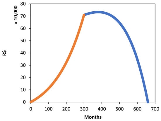
Figure 1. The orange series shows the evolution of the accumulated amount during the 25-year deposit period. After this phase, the blue series still indicates growth in the capital up to the seventh year of withdrawals. This occurs because, during that time, the investment returns continue to exceed the withdrawal amounts. From the eighth year onward, the capital begins to decline, reaching zero by the end of the thirtieth year of withdrawals.

3.1. Alternative Scenario (Historical IPCA Average 6.2%)

Using the same settings adopted in the baseline example (0.5% monthly interest rate, 25-year accumulation phase, and 30 years of withdrawals) and indexing annual deposits and benefits by the historical Brazilian inflation rate of 6.2% (IPCA average), the first-year benefit at retirement is:

$$S_1=1500(1+0.062{)}^{25}=6748.45$$

From Equation (4), the present value of the indexed withdrawal stream over 30 years is:

$$V_0=\mathrm{2,362,674.48}$$

Equating $V_0$ to the accumulation formula in Equation (3) yields the required first-year deposit:

$$D_1=1815.08$$

with annual 6.2% indexation of deposits.

This alternative scenario confirms that the model remains mathematically stable and easily recalibrated under historical Brazilian inflation conditions, thereby addressing concerns regarding potential divergence when realistic inflation rates are applied. Furthermore, it demonstrates that purchasing power is preserved by construction, without altering the model’s closed-form structure or ease of application.

3.2. Limitations and Possible Extensions

Although the proposed model offers a transparent and accessible framework for retirement planning, some limitations must be acknowledged. First, it is a deterministic formulation, which does not incorporate market risk or stochastic variation in parameters such as interest and inflation rates. Second, it assumes constant rates within each simulation horizon, which may not reflect real-world fluctuations. Third, taxation, administrative fees, and potential regulatory changes are not considered. Fourth, the initial calibration of the model—the determination of the first point—must be performed manually by the individual or institution applying it, which requires careful parameter selection.

Potential extensions of the model include incorporating stochastic scenarios for interest and inflation rates, adapting it to contexts with unstable or dollarized currencies, and applying it in different countries with parameter adjustments reflecting local economic realities. Furthermore, the model could be integrated into hybrid public–private pension systems or extended to account for taxation and transaction costs, enhancing its realism and policy relevance.

3.3. Sensitivity Analysis

To assess the robustness of 7 the proposed model, we conducted a sensitivity analysis varying the annual inflation correction rate. Table 4 below presents the initial monthly deposit $D$ required to achieve a retirement income of R$ 3049.19 (adjusted annually) for 30 years, assuming a constant monthly interest rate of 0.5% and a 25-year accumulation period:

Table 4. Sensitivity analysis of the required initial monthly deposit (D) as a function of different annual inflation rates, assuming a constant monthly interest rate of 0.5%, a 25-year accumulation period, and a retirement income goal of R$ 3049.19 (adjusted annually) over 30 years.

Annual Inflation Rate	Required Initial Deposit (R$)
2%	707.24
3%	767.67
4%	836.91

As expected, higher inflation rates demand greater initial deposits in order to preserve the same purchasing power during retirement. This analysis highlights the importance of accurate inflation forecasting in retirement planning.

4. Modeling Perpetual Pension Streams with Indexed Geometric Annuities

To obtain a perpetual income $\left(V_p\right)$, we let $n\to \mathrm{\infty }.$ This implies that in Equation (4), the expression $\left(\gamma \right)$ simplifies to calculating the sum of the terms of an infinite geometric progression, which gives us, with $0<q<1$:

$$\begin{gathered} V_p=\gamma S_1\left[{\displaystyle \frac{{\left(1+i\right)}^{12}-1}{i{\left(1+i\right)}^{12}}}\right] \\ =\left[{\displaystyle \frac{1}{1-\frac{1+i_r}{{\left(1+i\right)}^{12}}}}\right]S_1\left[{\displaystyle \frac{{\left(1+i\right)}^{12}-1}{i{\left(1+i\right)}^{12}}}\right] \\ =S_1\left[{\displaystyle \frac{{\left(1+i\right)}^{12}}{{\left(1+i\right)}^{12}-\left(1+i_r\right)}}\right]\left[{\displaystyle \frac{{\left(1+i\right)}^{12}-1}{i{\left(1+i\right)}^{12}}}\right] \\ =S_1\left\{{\displaystyle \frac{{\left(1+i\right)}^{12}-1}{i\left[{\left(1+i\right)}^{12}-\left(1+i_r\right)\right]}}\right\} \end{gathered}$$

(7)

$S_1$ is the withdrawal amount in the first year of retirement, $i$ is the interest rate of the investment, and $i_r$ is the geometric annuity percentage applied to the amount of the lifetime benefit. From Equation (7), for the same problem, with a lifetime income, we have:

$$V_p=3049.19\left[{\displaystyle \frac{{1.005}^{12}-1}{0.005({1.005}^{12}-1.03)}}\right]=R\$\mathrm{1,187,376.00}$$

By setting $V_p=M_T\Rightarrow D_1=R\$ 1285.93$. Now, if the withdrawals are always adjusted while the interest rate remains constant, how will my capital behave during the withdrawal period? The fund will continue to grow over time, even with inflation-adjusted withdrawals, as the returns will always exceed the withdrawal amount during the period. In Figure 2, by assigning values smaller than $V_p$, we observe that the amount reaches zero after a certain period of withdrawals, while for values greater than or equal to $V_p$, the balance grows over time.

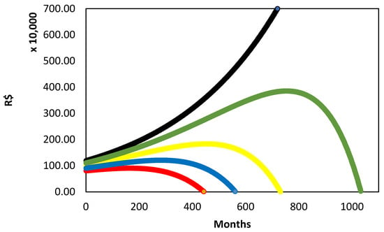
Figure 2. Balance during the withdrawal period. Amounts of $R\$ \mathrm{800,000.00}, R\$ \mathrm{900,000.00}, R\$ \mathrm{1,000,000.00}, R\$ \mathrm{1,100,000.00},$ and $Vp = R\$ \mathrm{1,187,376.00}$, in this order, from bottom to top. Red, blue, yellow, green, and black lines, respectively.

Note that this time frame is entirely out of context for our lifetime. For example, with an amount of $R\$ \mathrm{1,100,000.00}$, it would take 86 years of withdrawals to deplete the balance, which I would consider practically impossible for someone to reach such a period relying solely on retirement income. In the case of the amount $V_p=R\$ \mathrm{1,187,376.00}$, for a lifetime income, it does not seem financially reasonable to project deposits aiming for this balance, unless the goal is to leave an inheritance or to safeguard against life’s eventualities, which may require sporadic and considerable withdrawals from the accumulated capital. In this sense, the lifetime income presented here could become plausible or, at least, the initial projection of accumulating an amount between the calculated values, meaning that even with occasional unplanned withdrawals, the initial goal could remain achievable.

If inflation exceeds the monthly interest rate (e.g., 6% annual inflation vs. 0.3% monthly interest), the model still allows for projections, but it may require recalibration of the contribution plan to maintain the purchasing power goal. This reinforces the importance of periodic reviews and flexible adjustments in long-term financial planning.

5. Conclusions

This paper proposes a mathematical model based on modified geometric progressions for supplementary retirement planning. Unlike traditional annuity models that assume fixed contributions and withdrawals, the proposed method incorporates inflation-indexed inputs throughout both accumulation and decumulation phases. This refinement allows for more accurate simulations aligned with real-world financial dynamics. The model has practical applicability in pension fund policy design, personal financial planning tools, and governmental projections. A case study demonstrates that, with a 3% annual geometric annuity and a 0.5% monthly interest rate, an initial deposit of $R\$ 767.67$ over 25 years yields a monthly retirement income of $R\$ 3049.19$ for 30 years, maintaining purchasing power. The model thus provides a practical and realistic framework for retirement planning and supports future applications in both public and private pension systems.

This study proposed an innovative mathematical model for supplementary retirement planning, incorporating a geometric annuity index applied to both contributions and withdrawals. By adapting classical financial mathematics formulas and introducing a periodic correction factor, the model proved effective in preserving the beneficiary’s purchasing power over time, offering a more realistic alternative for economies with a history of significant inflation, such as Brazil.

Unlike traditional models that overlook the cumulative effects of inflation on future income, the approach presented here provides a mathematically consistent structure aligned with recent empirical and theoretical findings in the literature. Studies by Liu et al. [2] and Shao et al. [4] highlight the need for pension models that account for inflationary dynamics and wage volatility, while Martinez et al. [3] demonstrate that neglecting to index retirement benefits often leads to economic shortfalls with direct consequences on retirees’ well-being.

Moreover, current data on contributor behavior under inflationary pressure—as evidenced by surveys from the TIAA Institute [6] and Allianz Life [7]—reveal a growing demand for more resilient and transparent financial planning tools. The proposed model addresses this demand by offering mathematical clarity, practical feasibility, and direct applicability to individual or institutional retirement simulations.

The model mathematically demonstrates that a contribution plan starting with an initial deposit of R$ 767.67 (adjusted annually by 3%) and earning a monthly interest rate of 0.5% can provide a lifetime monthly income of R$ 3049.19 for thirty years, with purchasing power preserved. This approach offers tangible benefits: for investors, it ensures financial predictability with built-in inflation protection; for policymakers, it provides a quantitative tool for evaluating pension reform; and for financial professionals, it presents a replicable and adaptable methodology for planning tools.

Although the assumption of fixed rates represents a limitation—requiring periodic reassessment in volatile economic environments—the model establishes a solid foundation for future developments. These may include incorporating Brazilian historical data and stochastic techniques to enhance its robustness against real market fluctuations.

In conclusion, the introduction of a geometric annuity index represents a significant advancement in the field of financial mathematics applied to retirement planning. It enables the development of more realistic and sustainable strategies tailored to long-term individual needs. Future research may explore the integration of this model with stochastic inflation scenarios, broader public and private pension schemes, and its adaptation to diverse international fiscal and demographic contexts. While the current model assumes fixed rates and omits mortality, early withdrawal, and taxation factors, it serves as a tractable and implementable framework. Recognizing the value of stochastic modeling, we identify it as a critical direction for future refinement.

Future work will include calibrating the model with historical Brazilian inflation and wage data, and simulating stochastic environments using Monte Carlo methods.

Appendix A.1. Accumulation Period

$$\begin{gathered} M_T={M\prime }_1+{M\prime }_2+\dots +{M\prime }_{n-1}+M_n \\ M_T=D_1\left[{\displaystyle \frac{{\left(1+i\right)}^{12}-1}{i}}\right]{\left(1+i\right)}^{12\left(n-1\right)}+D_2\left[{\displaystyle \frac{{\left(1+i\right)}^{12}-1}{i}}\right]{\left(1+i\right)}^{12\left(n-2\right)}+\dots +D_{n-1}\left[{\displaystyle \frac{{\left(1+i\right)}^{12}-1}{i}}\right]\left(1+i\right)+D_n\left[{\displaystyle \frac{{\left(1+i\right)}^{12}-1}{i}}\right] \\ =\left[{\displaystyle \frac{{\left(1+i\right)}^{12}-1}{i}}\right]\left[D_1{\left(1+i\right)}^{12\left(n-1\right)}+D_2{\left(1+i\right)}^{12\left(n-2\right)}+\dots +D_{n-1}\left(1+i\right)+D_n\right] \\ =\left[{\displaystyle \frac{{\left(1+i\right)}^{12}-1}{i}}\right]\left[D_1{\left(1+i\right)}^{12\left(n-1\right)}+D_1\left(1+i_r\right){\left(1+i\right)}^{12\left(n-2\right)}+\dots +D_1{\left(1+i_r\right)}^{n-2}{\left(1+i\right)}^{12}+D_1{\left(1+i_r\right)}^{n-1}\right] \\ =D_1\left[{\displaystyle \frac{{\left(1+i\right)}^{12}-1}{i}}\right]\stackrel{\mathsf{\Psi }}{\overbrace{\left[{\left(1+i\right)}^{12\left(n-1\right)}+\left(1+i_r\right){\left(1+i\right)}^{12\left(n-2\right)}+\dots +{\left(1+i_r\right)}^{n-2}{\left(1+i\right)}^{12}+{\left(1+i_r\right)}^{n-1}\right]}} \end{gathered}$$

(A1)

Note that in Equation (A1), the expression $\left(\mathsf{\Psi }\right)$ denotes the sum of the terms of a geometric progression with first term $a_1={\left(1+i\right)}^{12\left(n-1\right)}$ and common ratio $q={\displaystyle \frac{1+i_r}{{\left(1+i\right)}^{12}}}$, whose sum is given by:

$$\begin{gathered} \mathsf{\Psi }={\left(1+i\right)}^{12\left(n-1\right)}\left[{\displaystyle \frac{{\left(\frac{1+i_r}{{\left(1+i\right)}^{12}}\right)}^n-1}{\frac{1+i_r}{{\left(1+i\right)}^{12}}-1}}\right] \\ ={\left(1+i\right)}^{12\left(n-1\right)}\left[{\displaystyle \frac{\frac{{\left(1+i_r\right)}^n}{{\left(1+i\right)}^{12n}}-1}{\frac{1+i_r-{\left(1+i\right)}^{12}}{{\left(1+i\right)}^{12}}}}\right] \\ ={\left(1+i\right)}^{12\left(n-1\right)}\left[{\displaystyle \frac{\frac{{\left(1+i_r\right)}^n-{\left(1+i\right)}^{12n}}{{\left(1+i\right)}^{12n}}}{\frac{1+i_r-{\left(1+i\right)}^{12}}{{\left(1+i\right)}^{12}}}}\right] \\ ={\left(1+i\right)}^{12\left(n-1\right)}\left[{\displaystyle \frac{{\left(1+i_r\right)}^n-{\left(1+i\right)}^{12n}}{{\left(1+i\right)}^{12n}}}\right]\left[{\displaystyle \frac{{\left(1+i\right)}^{12}}{{1+i_r-\left(1+i\right)}^{12}}}\right] \\ ={\displaystyle \frac{{\left(1+i_r\right)}^n-{\left(1+i\right)}^{12n}}{\left(1+i_r\right)-{\left(1+i\right)}^{12}}} \end{gathered}$$

(A2)

Finally, substituting Equation (A2) into Equation (A1), we obtain the total amount with the following expression:

$$\begin{gathered} M_T=D_1\left[{\displaystyle \frac{{\left(1+i\right)}^{12}-1}{i}}\right]\mathsf{\Psi } \\ =D_1\left\{{\displaystyle \frac{{[\left(1+i\right)}^{12}-1\left]\right[{\left(1+i_r\right)}^n-{\left(1+i\right)}^{12n}]}{i\left[\left(1+i_r\right)-{\left(1+i\right)}^{12}\right]}}\right\} \end{gathered}$$

(A3)

Appendix A.2. Withdrawal Period

$$\begin{array}{l} V_0=V_1+{V\prime }_2+{V\prime }_3+{V\prime }_4+\dots +{V\prime }_{n-1}+{V\prime }_n\\ =S_1\left[{\displaystyle \frac{{\left(1+i\right)}^{12}-1}{i{\left(1+i\right)}^{12}}}\right]+{\displaystyle \frac{S_2}{{\left(1+i\right)}^{12}}}\left[{\displaystyle \frac{{\left(1+i\right)}^{12}-1}{{i\left(1+i\right)}^{12}}}\right]+{\displaystyle \frac{S_3}{{\left(1+i\right)}^{2\left(12\right)}}}\left[{\displaystyle \frac{{\left(1+i\right)}^{12}-1}{{i\left(1+i\right)}^{12}}}\right]+{\displaystyle \frac{S_4}{{\left(1+i\right)}^{3\left(12\right)}}}\left[{\displaystyle \frac{{\left(1+i\right)}^{12}-1}{{i\left(1+i\right)}^{12}}}\right]+\dots +{\displaystyle \frac{S_{n-1}}{{\left(1+i\right)}^{12(n-1)}}}\left[{\displaystyle \frac{{\left(1+i\right)}^{12}-1}{{i\left(1+i\right)}^{12}}}\right]+{\displaystyle \frac{S_n}{{\left(1+i\right)}^{12n}}}\left[{\displaystyle \frac{{\left(1+i\right)}^{12}-1}{{i\left(1+i\right)}^{12}}}\right]\\ =S_1\left[{\displaystyle \frac{{\left(1+i\right)}^{12}-1}{i{\left(1+i\right)}^{12}}}\right]+{\displaystyle \frac{S_1\left(1+i_r\right)}{{\left(1+i\right)}^{12}}}\left[{\displaystyle \frac{{\left(1+i\right)}^{12}-1}{{i\left(1+i\right)}^{12}}}\right]+{\displaystyle \frac{S_1{\left(1+i_r\right)}^2}{{\left(1+i\right)}^{2\left(12\right)}}}\left[{\displaystyle \frac{{\left(1+i\right)}^{12}-1}{{i\left(1+i\right)}^{12}}}\right]+{\displaystyle \frac{S_1{\left(1+i_r\right)}^3}{{\left(1+i\right)}^{3\left(12\right)}}}\left[{\displaystyle \frac{{\left(1+i\right)}^{12}-1}{{i\left(1+i\right)}^{12}}}\right]+\dots +{\displaystyle \frac{S_1{\left({1+i}_r\right)}^{n-2}}{{\left(1+i\right)}^{(n-2)12}}}\left[{\displaystyle \frac{{\left(1+i\right)}^{12}-1}{{i\left(1+i\right)}^{12}}}\right]+{\displaystyle \frac{S_1{\left({1+i}_r\right)}^{n-1}}{{\left(1+i\right)}^{\left(n-1\right)12}}}\left[{\displaystyle \frac{{\left(1+i\right)}^{12}-1}{{i\left(1+i\right)}^{12}}}\right]\\ =S_1\left[{\displaystyle \frac{{\left(1+i\right)}^{12}-1}{i{\left(1+i\right)}^{12}}}\right]\stackrel{\gamma }{\overbrace{\left[1+{\displaystyle \frac{1+i_r}{{\left(1+i\right)}^{12}}}+{\displaystyle \frac{{\left(1+i_r\right)}^2}{{\left(1+i\right)}^{2\left(12\right)}}}+{\displaystyle \frac{{\left(1+i_r\right)}^3}{{\left(1+i\right)}^{3\left(12\right)}}}+\dots +{\displaystyle \frac{{\left(1+i_r\right)}^{n-2}}{{\left(1+i\right)}^{12\left(n-2\right)}}}+{\displaystyle \frac{{\left(1+i_r\right)}^{n-1}}{{\left(1+i\right)}^{12(n-1)}}}\right]}}\end{array}$$

(A4)

It is easy to see that in Equation (A4), the expression $\left(\gamma \right)$ represents the sum of the terms of a geometric progression with the first term $a_1=1$ and common ratio $q={\displaystyle \frac{1+i_r}{{\left(1+i\right)}^{12}}}$, whose sum is given by:

$$\begin{gathered} \gamma ={\displaystyle \frac{{\left[\frac{\left(1+i_r\right)}{{\left(1+i\right)}^{12}}\right]}^n-1}{\left[\frac{1+i_r}{{\left(1+i\right)}^{12}}\right]-1}} \\ ={\displaystyle \frac{\frac{{\left(1+i_r\right)}^n-{\left(1+i\right)}^{12n}}{{\left(1+i\right)}^{12n}}}{\frac{1+i_r-{\left(1+i\right)}^{12}}{{\left(1+i\right)}^{12}}}} \\ =\left[{\displaystyle \frac{{\left(1+i_r\right)}^n-{\left(1+i\right)}^{12n}}{{\left(1+i\right)}^{12n}}}\right]\left[{\displaystyle \frac{{\left(1+i\right)}^{12}}{1+i_r-{\left(1+i\right)}^{12}}}\right] \end{gathered}$$

(A5)

therefore, the Present Value $\left(V_0\right)$ of the set of withdrawals $S_j$, by substituting Equation (A5) into Equation (A4), is the following expression:

$$\begin{gathered} V_0=\gamma S_1\left[{\displaystyle \frac{{\left(1+i\right)}^{12}-1}{i{\left(1+i\right)}^{12}}}\right] \\ =S_1\left[{\displaystyle \frac{{\left(1+i_r\right)}^n-{\left(1+i\right)}^{12n}}{{\left(1+i\right)}^{12n}}}\right]\left[{\displaystyle \frac{{\left(1+i\right)}^{12}}{1+i_r-{\left(1+i\right)}^{12}}}\right]\left[{\displaystyle \frac{{\left(1+i\right)}^{12}-1}{i{\left(1+i\right)}^{12}}}\right] \\ =S_1\left\{{\displaystyle \frac{\left[{\left(1+i\right)}^{12}-1\right]\left[{\left(1+i_r\right)}^n-{\left(1+i\right)}^{12n}\right]}{i{\left(1+i\right)}^{12n}\left[1+i_r-{\left(1+i\right)}^{12}\right]}}\right\} \end{gathered}$$

(A6)

References

- Foziah, H.; Afthanorhan, A.; Ghazali, P.L.; Tajuddin, S.A.F.S. Impact of inflation severity on retirement savings: A simulation analysis of projected accumulation and de-accumulation. J. Soc. Econ. Res. 2023, 10, 124–133. [Google Scholar] [CrossRef]
- Liu, S.; Wang, C.; Xue, J. Valuation of Hybrid Pension Scheme Liabilities under Inflation. Wuhan Univ. J. Nat. Sci. 2022, 27, 153–160. [Google Scholar] [CrossRef]
- Costa-Font, J.; Vilaplana-Prieto, C. Caregiving subsidies and spousal early retirement intentions. J. Pension Econ. Financ. 2023, 22, 550–589. [Google Scholar] [CrossRef]
- Shao, Y.; Xia, D.; Fei, W. Optimal investment strategy for DC pension plan with inflation risk under the hybrid stochastic volatility model. Syst. Sci. Control Eng. 2023, 11, 2186962. [Google Scholar] [CrossRef]
- Wang, J.; Li, Y. Optimal pension investment under wage uncertainty and inflation: A time-consistent approach. J. Econ. Dyn. Control 2022, 144, 192–211. [Google Scholar] [CrossRef]
- TIAA Institute; GFLEC. Inflation Forces 1 in 4 Americans to Cut Retirement Savings. 2023. Available online: https://www.tiaa.org/public/institute/about/news/inflation-forces-1-in-4-americans-to-cut-retirement-savings (accessed on 1 June 2025).
- Allianz Life Insurance Company of North America. Inflation Causing Majority of Americans to Stop or Reduce Retirement Savings. 2022. Available online: https://www.businesswire.com/news/home/20221026005249/en/Inflation-Causing-Majority-of-Americans-to-Stop-or-Reduce-Retirement-Savings (accessed on 1 June 2025).
- Tiong, S. Pricing inflation-linked variable annuities under stochastic interest rates. Insur. Math. Econ. 2013, 52, 77–86. [Google Scholar] [CrossRef]
- Mataramvura, S. Valuation of inflation-linked annuities in a Lévy market. J. Appl. Math. 2011, 2011, 897954. [Google Scholar] [CrossRef]
- Montufar-Benítez, M.A.; Dávalos-Argandoña, C.; Velasco, S. An Actual Case Study of a Deterministic Multi-Objective Optimization Model in a Defined Contribution Faculty Pension System. Computation 2025, 13, 25. [Google Scholar] [CrossRef]
- Wang, Y.; Xu, X.; Zhang, J. Optimal Investment Strategy for DC Pension Plan with Stochastic Income and Inflation Risk under the Ornstein–Uhlenbeck Model. Mathematics 2021, 9, 1756. [Google Scholar] [CrossRef]
- Donnelly, C.; Khemka, G.; Limb, W. Money Illusion in Retirement Savings with a Minimum Guarantee. Scand. Actuar. J. 2024, 2024, 225–245. [Google Scholar] [CrossRef]
- Barucci, E.; Marazzina, D. Optimal Investment, Stochastic Labor Income and Retirement. Appl. Math. Comput. 2012, 218, 5588–5604. [Google Scholar] [CrossRef]
- Silva, C.G.d.; Leme, M.C.d.S. An analysis of the degrees of persistence of inflation, inflation expectations and real interest rate in Brazil. Rev. Bras. Econ. 2011, 65, 289–302. [Google Scholar] [CrossRef]
- França, L.H.F.; Hershey, D.A. Financial Preparation for Retirement in Brazil: A Cross-Cultural Test of the Interdisciplinary Financial Planning Model. J. Cross-Cult. Gerontol. 2018, 33, 43–64. [Google Scholar] [CrossRef] [PubMed]
- Muralidhar, A.; Vitorino, A.A. How Brazil’s RendA+ Bond Could Render DC Retirement Risk Obsolete: A Case Study; Working paper; SSRN: Rochester, NY, USA, 2025. [Google Scholar] [CrossRef]
- Previ. Annual Report 2022: Plan 1—Profitability and Results. Previ. 2023. Available online: https://previ2022.blendon.com.br/wp-content/uploads/2023/05/previ_RA_2022_PT_985x600px_AF-v1.pdf (accessed on 7 August 2025).
- BRAZIL. Ordinance No. 8, Dated January 13, 2017. Provides for the Adjustment of Benefits Paid by the National Institute of Social Security (INSS) and Other Amounts Listed in the Social Security Regulation. Available online: http://pesquisa.in.gov.br/imprensa/jsp/visualiza/index.jsp?data=16/01/2017&jornal=1&pagina=12&totalArquivos=68 (accessed on 24 April 2025).
- Lima, E.L.; Carvalho, P.C.P.; Wagner, E.; Morgado, A.C. Temas e Problemas; SBM: Rio de Janeiro, Brazil, 2010. [Google Scholar]
- Iezzi, G.; Hazzan, S.; Degenszajn, D. Fundamentos de Matemática Elementar Volume 11: Matemática Comercial; Matemática financeira e Estatística descritiva; Atual: São Paulo, Brazil, 2013. [Google Scholar]
- Hazzan, S. Poupando Para a Aposentadoria; RPM 33; SBM: Rio de Janeiro, Brazil, 2017; Available online: https://rpm.org.br/cdrpm/33/2.htm (accessed on 24 April 2025).
- Blake, D.; Cairns, A.J.G.; Dowd, K. Pensionmetrics 2: Stochastic pension plan design during the distribution phase. Insur. Math. Econ. 2003, 33, 29–47. [Google Scholar] [CrossRef]
- Gerrard, R.; Haberman, S.; Vigna, E. Optimal investment choices post-retirement in a defined contribution pension scheme. Insur. Math. Econ. 2004, 35, 321–342. [Google Scholar] [CrossRef]
- Milevsky, M.A.; Salisbury, T.S. Financial valuation of guaranteed minimum withdrawal benefits. Insur. Math. Econ. 2006, 38, 21–38. [Google Scholar] [CrossRef]
Disclaimer/Publisher’s Note: The statements, opinions and data contained in all publications are solely those of the individual author(s) and contributor(s) and not of MDPI and/or the editor(s). MDPI and/or the editor(s) disclaim responsibility for any injury to people or property resulting from any ideas, methods, instructions or products referred to in the content. |
© 2025 by the authors. Licensee MDPI, Basel, Switzerland. This article is an open access article distributed under the terms and conditions of the Creative Commons Attribution (CC BY) license (https://creativecommons.org/licenses/by/4.0/).