Quantization of Faster R-CNN Quantization of Faster R-CNN

Abstract

The Faster Region-based Convolutional Network (Faster R-CNN) is an efficient object detection model. However, its large size and significant computational requirements limit its applicability in embedded systems and real-time environments. Quantization is a proven method for reducing models’ size and computational requirements, but there is currently no open-source general implementation for quantizing Faster R-CNN. The main reason is that individual architecture components need to be quantized separately due to their structural characteristics. We present a general Faster R-CNN quantization algorithm, for which our implementation is open-source and compatible with the PyTorch (2.7.0+cu126, pt12) ecosystem. Our solution reduces the model size by 67.2% and the detection time by 50.4% while maintaining the accuracy measured on the test data within an error margin of 8.2% and a standard deviation of ±3.4%. It also allows for the visualization of model errors by extracting the model’s internal activation maps, supporting a more efficient understanding of its behavior. We demonstrate that the proposed method can effectively quantize Faster R-CNN, enabling the model to run on low-power hardware. This is particularly important in applications such as autonomous vehicles, embedded sensor systems, and real-time security surveillance, where fast and energy-efficient object detection is crucial.

1. Introduction

Convolutional neural networks (CNNs) have evolved into complex, multi-layered architectures that can not only efficiently solve image classification tasks but also provide practical answers to the problem of object detection and localization. That is particularly important in real-time applications such as self-driving vehicles, intelligent surveillance systems, or medical image analysis, where accuracy and fast recognition beyond human capabilities are key.

Faster R-CNN (Region-based Convolutional Neural Network [1], YOLO (You Only Look Once) [2], and Vision Transformer [3] are just a few examples of these complex architectures. However, the complexity of these models increases the computational demand and, therefore, limits their application in embedded and mobile systems. That is addressed by quantization, which converts floating-point numbers used by the IEEE 754 fp32 (floating point) [4] standard into lower bit-depth representations (fp16, fp8) [5] or transforms them into integers (int8, int4) [6]. Integer numbers also provide faster hardware operations. Although quantization does not necessarily result in a significant performance degradation in accuracy, as tested and described by researchers [7,8], the modified number representation significantly improves prediction speed. The quantized model is mainly used for inference, which is how hundreds of frames per second can be achieved for a CNN.

Each environment has its quantization libraries (TensorRT, ONNX, PyTorch, TensorFlow); Torch’s documentation [9] summarizes the possibilities well. Another problem is that these different libraries are not compatible with each other.

There is currently no publicly available library for quantizing the Faster R-CNN complex neural network. The architecture can be dynamically quantized, but this does not apply to the convolutional layers [9]. Our goal in quantizing the Faster R-CNN is to minimize runtime, optimize for hardware, and provide a generalized quantization of the Faster R-CNN that allows us to monitor its internal outputs (via hooks) [10], making it suitable for error measurement. The error measurement will allow us to apply different quantization strategies and learn more about good quantization methods in a hardware-optimized environment. Deep learning frameworks such as Torch or TensorFlow are suitable for this. We chose PyTorch (2.7.0+cu126, pt12) because it is more actively evolving regarding trends [11], and hence, we assume more stability.

In the following sections of our paper, we present our generalized quantization solution for the Faster R-CNN neural network and its main results. In Section 2, Research Methods, we describe in detail how and according to which methodology we designed the generalized algorithm and how we evaluated its efficiency. In the Result and Discussion Section 3, we describe the results of our algorithm and the further implications of our development for architectures using complex convolutional networks of the Faster R-CNN. Finally, in the Conclusion Section 4, we summarize the main contributions of our research and development work to the field.

2. Research Methods

In Data Section 2.1, we present the labeled dataset used for training, which is also used for quantization and calibration. In Section 2.2, we present the ResNet [12] and Faster R-CNN architectures and their generalized quantization steps.

2.1. Data

We used the KITTI [13,14] dataset to test our quantization algorithm. KITTI is one of the most well-known and widely used real-world benchmark datasets for computer vision tasks related to autonomous vehicles. The dataset is primarily intended to support research on self-driving systems.

KITTI includes several subsets for different tasks (e.g., visual odometry, stereo vision, tracking, 3D reconstruction), but we used the “Object Detection” part. This subset of the KITTI contains 7481 frames for teaching and 7518 frames for testing, all captured with a calibrated camera system mounted on a vehicle windshield. The essential object classes are Car, Van, Truck, Pedestrian, Cyclist, Tram, Misc, Person_sitting, and DontCare. The annotations, including the object category and its 2D bounding box, are hand-labeled.

This rich, accurately annotated dataset allows thorough testing of object detection algorithms, focusing on classification and localization performance. As it contains motion-captured images from real-world environments under a variety of lighting conditions and scenes, KITTI is particularly well-suited for testing methods aimed at practical applications of deep neural networks, such as quantized models, in resource-constrained environments such as embedded hardware for self-driving systems.

2.2. Generalized Method

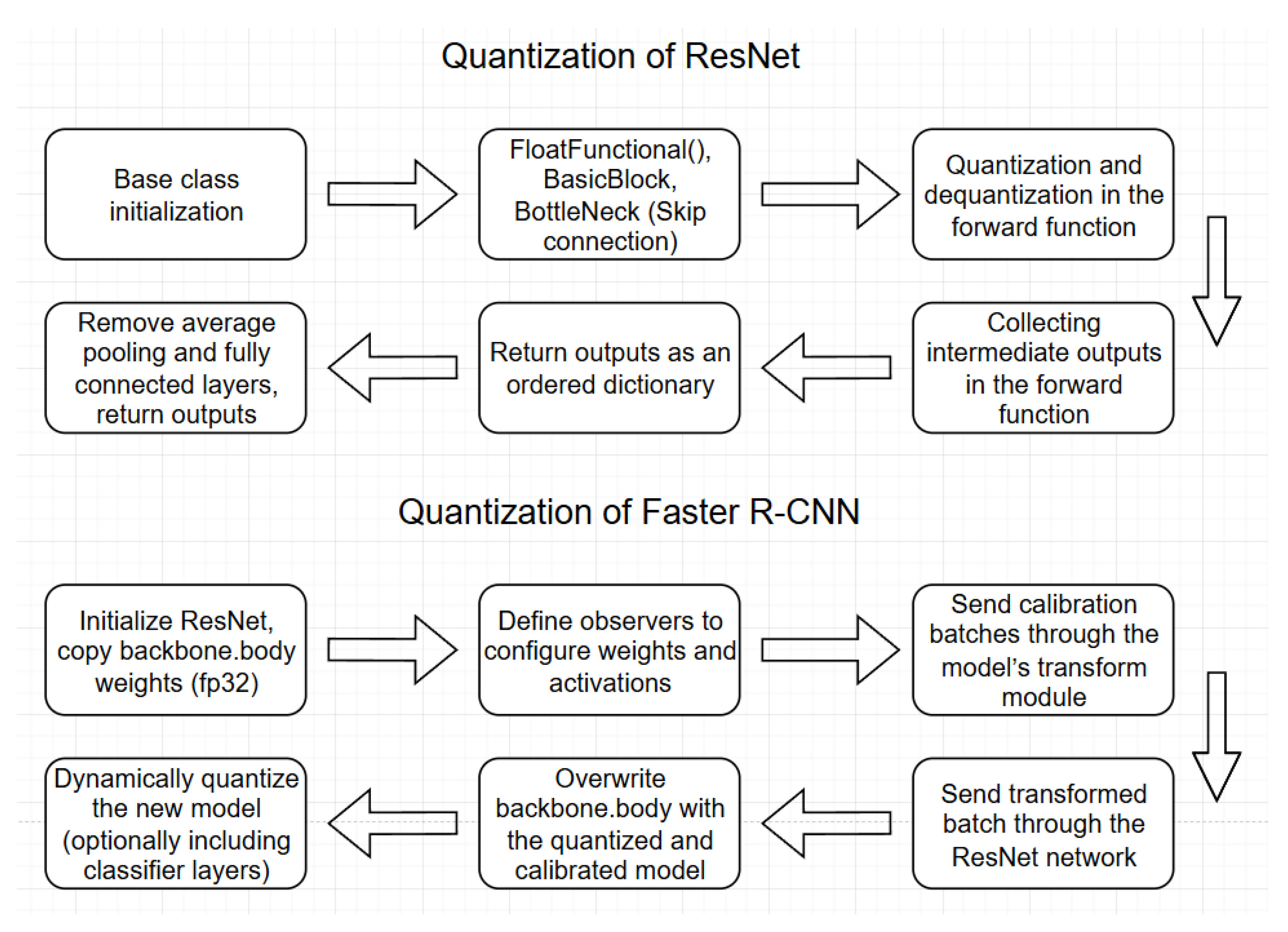
We used a version of the Faster R-CNN complex neural network architecture, ResNet50 [15], built on a CNN mesh to design the generalized quantization algorithm. Moreover, for an in-depth analysis of the quantization error, we did not rely only on classical metrics, but it became essential to investigate the internal part of the model. However, our model’s architecture poses challenges in quantizability and computation of gradients, which we had to consider when designing our algorithm. The workings of our generalized algorithm are detailed in Figure 1 (flowchart), and its complexity sheds light on the difficulties of solving these problems.

Figure 1. Transforming the quantizable ResNet and quantizing the Faster R-CNN.

Torchvision provides a quantizable ResNet implementation [16], which adds quantized operators to the skip connection part and performs QDQ quantization in the forward function. In our implementation [17], it is also necessary to collect internal feature maps in the forward functions for later object detection and removal of classifier layers. ResNet is preferred over other CNNs because of its skip connections [18], which help mitigate the vanishing gradient problem. However, alternative architectures could also be considered. Other CNNs are much simpler to quantize. These steps are described in the Table 1 and Table 2 below.

Table 1. Quantized ResNet.

#	Step	Code/Description
1	Initialize Quantized ResNet Base	super().__init__(block, layers, **kwargs)
2	Add QDQ and FloatFunctional support for skip connections	quantized_resnet.quant ← QuantStub() quantized_resnet.dequant ← DeQuantStub()   for block in [QuantizedBasicBlock, QuantizedBottleneck] block.skip_add ← FloatFunctional() Replace skip connection: out ← skip_add.add(out, identity) end for
3	Apply QDQ in the forward pass	x ← self.quant(x) outputs ← ForwardImpl(self, x)   For each key in outputs do outputs[key] ← self.dequant(outputs[key]) end for
4	Forward implementation: feature map extraction	ForwardImpl(model, x): x ← conv1 → bn1 → relu → maxpool o0 ← layer1(x) o1 ← layer2(o0) o2 ← layer3(o1) o3 ← layer4(o2)
5	Return output as OrderedDict	return OrderedDict{“0”: o0, “1”: o1, “2”: o2, “3”: o3}
6	Remove avgpool and classifier head	del quantized_resnet.avgpool del quantized_resnet.fc
7	Make a new ResNet instance	quantized_resnet ← QuantizedResNet( block = QuantizedBottleneck, layers = [3, 4, 6, 3] )

Table 2. Quantization of Faster R-CNN.

#	Step	Code/Description
1	Initialize quantizable ResNet	quantized_resnet ← QuantizableResNet50() weights ← GetWeights(model_fp32.backbone.body) LoadWeights(quantized_resnet, weights) SetEvalMode(quantized_resnet)
2	Define quantization observers	activation_observer ← HistogramObserver() weight_observer ← PerChannelWeightObserver() qconfig ← QConfig(activation_observer, weight_observer) SetQConfig(quantized_resnet, qconfig)
3	Prepare model for quantization	PrepareForQuantization(quantized_resnet)
4	Send calibration data through the transform module	for each images in data_loader do    transformed ← TransformImages(model_fp32, images)    inputs ← GetTensors(transformed)    RunForward(quantized_resnet, inputs) end for
5	Replace the fp32 model’s backbone	ConvertToQuantizedModel(quantized_resnet) SetEvalMode(quantized_resnet) model_quantized ← DeepCopy(model_fp32) model_quantized.backbone.body ← quantized_resnet
6	Apply dynamic quantization	DynamicQuantize(model_quantized)

The tables present the quantization process’s step-by-step logic using pseudocode. The “Step” column concisely describes each major operation, while the “Code” column shows the corresponding implementation logic in Python-like syntax. This format was chosen to link each conceptual step with its low-level implementation, improving clarity for readers unfamiliar with the quantization pipeline. Using a table over plain text helps structure the pseudocode to emphasize the method’s sequential nature, making it easier to follow and reference later in the text.

ResNet consists of three main parts: the BasicBlock, Bottleneck, and the ResNet main class. The flowchart and the code show the latter. To support quantization, we need to add the FloatFunctional() function to the first two parts of ResNet (BottleNeck and BasicBlock). Compared to the original implementation, the results (feature maps) of the higher-level convolutions are collected in a dictionary and passed to a single dictionary after decanting to the next part of the Faster R-CNN, the FPN, in a classical CNN case, where the goal is a final classification. It is not necessary to keep the previous feature maps. However, for object detection and classification, feature maps of different sizes and levels are a good representation of sub-objects of various sizes. A higher-level convolution may detect the wheel; a lower-level convolution may combine these parts into an object.

To quantize in Table 2, we first need to initialize the quantizable ResNet network and copy the CNN weights in the Backbone Body part of the Faster R-CNN (still in fp32). Then, we need to define an observer; in the example, we have a distribution-based one, which computes the minima and maxima of the decanted values from the activations of the calibration images. The Backbone is not the first layer of the deep learning model; before it, there is a Transform module whose output will be received by the internal CNN, so the images are transformed with this. We calibrate the quantizable ResNet with these batches, and in the last step, we overwrite this module for the Faster R-CNN. Further quantization can then be performed on the linear layers.

The Torch supports hooks, so traceability is possible for both versions. In addition, hexbin plots can be used to cluster the differences in activations based on the activations of the original model, here it is not necessary to take the maxima of the channels, and any metric can be used, as will be demonstrated in Section 3, where we have plotted and examined absolute and relative (percentage) deviation graphs using our method. In addition, videos of DataLoader and DataLoader were also produced, showing the bounding boxes and feature maps of the two models. In addition, the QDQ quantization allows the use of int8 number representation.

3. Results and Discussion

3.1. Size and Accuracy

The results of our generalized algorithm in terms of size reduction and accuracy are as follows. Faster R-CNN is a deep learning model with a size of 159 MB. With implementations [17,19], the model size has been reduced by a third (53 MB), and its prediction time has been halved.

Regarding metrics in Table 3, the original model has an accuracy of 0.87 on test data, a precision of 0.79, and an mIoU of 0.84. The metrics for the quantized model are 0.74, 0.78, and 0.84. Of these, only the precision has dropped. For example, the YOLO model’s quantization algorithm does not even measure the accuracy of an object detection model [20]. In the case of YOLO, this can be considered a shortcoming compared to our solution.

Table 3. Comparison of quantization results using different calibration image quantities.

Metric	Original Model	INT8	INT8
Number of pictures	–	2 × 32	7500
Accuracy (%)	87.01	74.46	74.46
Precision (%)	78.72	77.83	77.13
Bounding box area (mIoU %)	84.46	83.00	83.19

3.2. Calibration

The calibration after quantization under the algorithm development resulted in the following observations. Several calibration methods were investigated, such as min-max addition, moving average, per channel, and finding the minimum and maximum values of int8/int16 based on the distribution. There is also an asymmetric version of the distribution-based approach, which allows the midpoint of the range to be other than 0.

That may be necessary because the step size is uniform, and floating-point numbers continuously increase. The smaller the interval, the smaller the step interval so you can get a more accurate result with the correct calibration. Thus, the distribution of activations can be calculated as input for real images.

There are more advanced quantization algorithms, such as AdaRound or AdaQuant (AMD Quark ONNX) [21], where memory is already finite. We observed that the whole training dataset is not nearly needed if the images are chosen correctly. Calibrating with 64 images resulted in a maximum $\pm 0.7$% change in the metrics compared to using the entire training dataset (7500), so there is an optimum for these numbers.

With fewer bits plotted, you need more int, and if you do not have enough, it will not predict well, but this is highly dataset and model-dependent.

Calibration is a critical part of mesh quantization because of the behavior of activations. For example, calibrating with a random tensor can reduce the accuracy to as low as 0% and render the model useless.

Finding the proper calibration method is also critical because the entire training dataset can have significant computational overhead and take longer than a learning epoch. However, for some data samples that are well represented in the variance of the dataset, one batch is enough for calibration, which is a kind of sampling from the distribution.

That is because the central limiting distribution theorem [22] states that the sample variance, distribution, and expected value will converge to the original data set, the formula for which is as follows:

$$Z_n={\displaystyle \frac{{\sum }_{i=1}^n{X}_i-\mu }{\sigma /\sqrt{n}}}$$

where $X_1,X_2,\dots ,X_n$ are independent and identically distributed random variables with finite mean $\mu$ and variance ${\sigma }^2$, then the normalized sum converges in distribution to a standard normal distribution $\mathcal{N}(0,1)$ as $n\to \infty$.

If only two batches or the whole training dataset were passed to the histogram-based observer for calibration, the following results were obtained, which are shown in Table 3.

As shown in Table 3, a few batches are enough to calibrate; if the sampling is correct, it is unnecessary to iterate over the whole dataset, and the previous theorem says so; it will not significantly improve the result. The optimal number of this varies.

3.3. Visualization of Activation Map

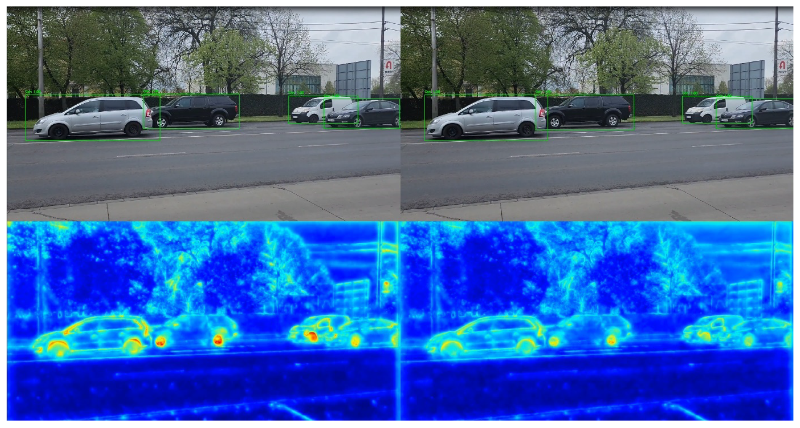
A further result of our algorithm’s operation is access to the model activation space image at a depth that allows efficient visualization of the following error between the quantized and the original model. Namely, to visualize the error, it is first necessary to visualize the activation maps of the original and the quantized model. By taking a maximum per channel, any layers of different sizes can simultaneously be compared per pixel and area, as we see in the next Figure 2, Figure 3, Figure 4 and Figure 5.

Figure 2. The original validation image with the quantized model. Green is the predicted box, red is the annotated box.

Figure 3. Maximum values of the first convolution channels with the quantized model.

Figure 4. Average of maxima of the first four convolution layers with the quantized model.

Figure 5. Average of the maxima of all CNN convolutions with the quantized model.

As seen in Figure 6, Figure 7, Figure 8 and Figure 9, after quantization, the difference (i.e., error) between the Faster R-CNN network and its quantized version can be measured and visualized layer by layer. The error distribution can be efficiently examined simultaneously for a given layer or several layers. We can define the difference metric (absolute, percentage, MSE, etc.).

Figure 6. Maximum activation errors for the first-level feature map.

Figure 7. Average differences across all layers between the two models.

Figure 8. Average differences for all strata, but proportionalised by percentage.

Figure 9. A prediction frame from an archive video (original model on the left).

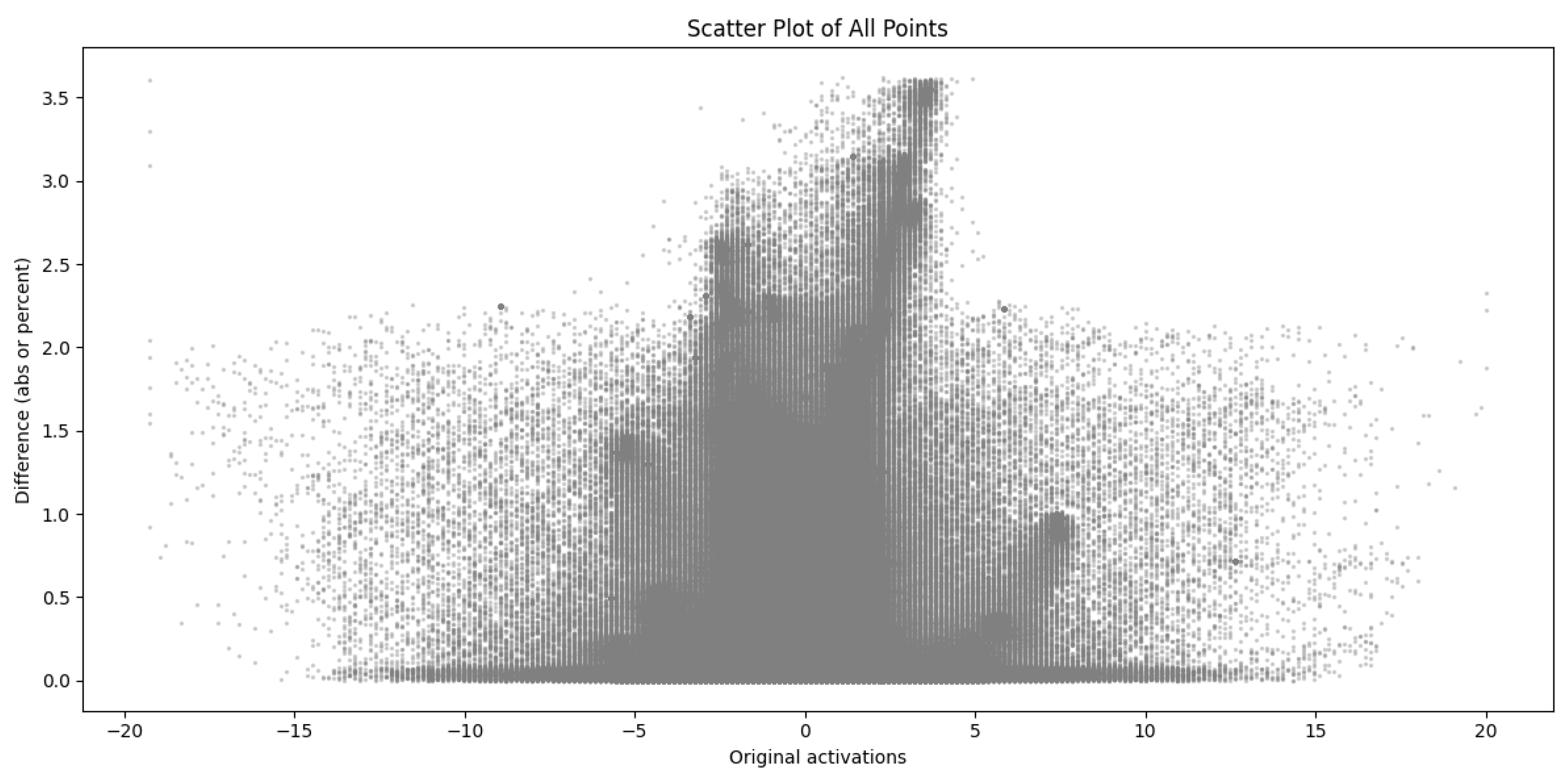
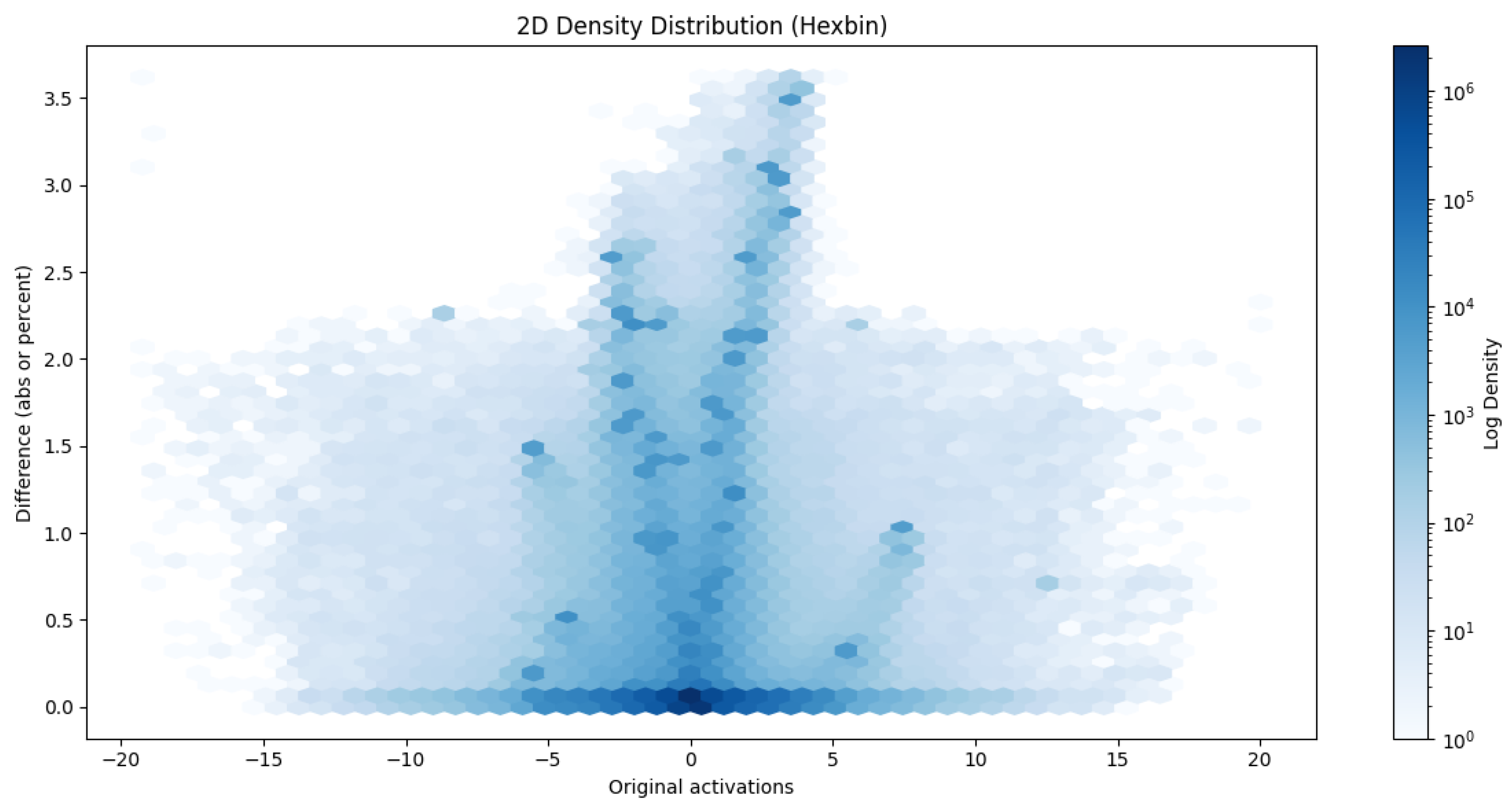
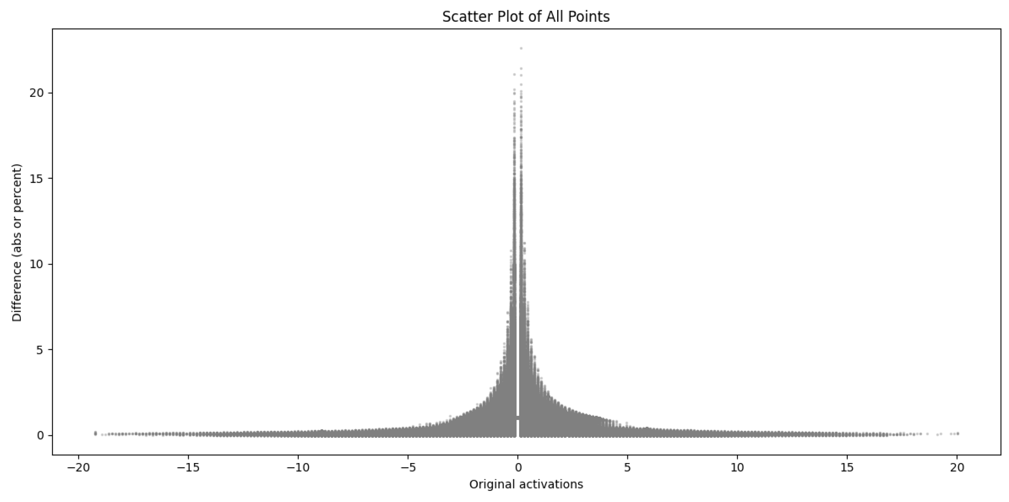
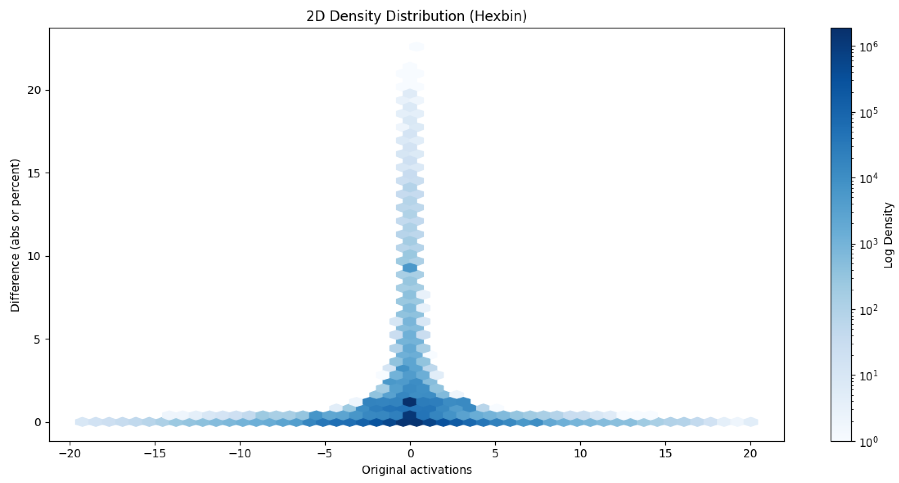
The error does not necessarily have to be grouped by pixel; we can also group by original activations and deviations from them, as shown in the following hexbins Figure 10 and Figure 11.

Figure 10. Absolute error values and their original activation function values.

Figure 11. Distribution of absolute errors by density between the two models.

The hexbin plots show the absolute errors of all convolution layers between the original and the quantized model, grouped by activations of the original model. In the case of convolution, the activations are densified over a small interval (most fall in the ±5 range, so the density of points is plotted on a logarithmic scale. A V-shape symmetric about the Y-axis is observed, indicating that higher activation values are associated with higher point-based errors. However, a horizontal line on the X-axis is also observed, which often implies an absolute error close to zero. Around the location x = 0, a less dense field is observed, indicating that when the original activation was close to 0, the step size of the floating point numbers is not uniform, but the quantized values are. That means that there is often a rounding error.

The other light blue parts of the hexbin graph represent scarce values, which can help choose the correct calibration data patterns. After all, for calibration, it is advisable to select samples that best describe the inputs that will occur in real life.

The tool can be used to calculate an error matrix with any metric. In this example (Figure 12 and Figure 13), we take relative deviations from each other based on the plots, which gives a much better indication of the errors for tiny numbers. The step size of floating-point numbers does not increase linearly, so the error rate bound decreases symmetrically about the Y axis to a low point. A rounding to 0.01 because of the uniform step size means a proportionally much larger inaccuracy for 0.1 than for 10. The area under the exponential curve fitted to the highest point and then mirrored in the given coordinates of the X-axis is not empty because the rounding sets a maximum for the error. As the step size of floating-point numbers increases, these errors become smaller and smaller.

Figure 12. Proportional differences in activation values between the two models.

Figure 13. Distribution of proportional errors based on density between the two models.

To summarize the previous statements, a minor percentage error at high activations can mean more in absolute terms because these will be the areas that the later layers will process; a low activation, in the case of convolution, does not pose such a big problem in later layers if we cannot represent it so accurately. Unlike linear layers, they are not connected to every neuron. The dimension reduction of max-pooling also reduces this error because it will leave the best-fitting sample, discarding the already low value. What matters more is how much the rounding error of the larger value was. However, a hex bin can also tell the error’s maximum, average, and other statistical metrics without looking for distributions.

4. Conclusions

In this study, we introduced a fully functional, generalized, and open-source quantization framework for the Faster R-CNN architecture. We specifically designed it for real-world applications to embedded systems, autonomous vehicles, and resource-constrained environments.

Our approach delivers a 67.2% reduction in model size and a 50.4% reduction in inference time while retaining a high level of accuracy, with an observed deviation of less than 8.2% compared to the original full-precision model.

Unlike prior efforts that exclude convolutional layers from quantization or offer only partial tooling, our method fully quantizes the entire pipeline—including the ResNet backbone—within the PyTorch ecosystem.

We also introduce an integrated strategy for capturing internal activation maps during inference, which enables transparent error analysis, traceability, and targeted model diagnostics. These features are especially valuable for safety-critical applications like automated driving or real-time surveillance, where interpretability and robustness are paramount.

Through extensive experimentation on the KITTI dataset, we demonstrate that calibration—often perceived as computationally expensive—can be effectively performed with a well-selected subset of just 64 images. That significantly lowers the barrier to deploying quantized models in practice, making our method viable even for workflows with strict latency, energy, or hardware constraints.

The accompanying visual analytics tools, including activation heatmaps and error distribution plots, provide actionable insights for optimizing quantization strategies. These tools allow engineers to tune performance trade-offs according to hardware targets and deployment contexts, such as int8 inference on edge accelerators or mixed-precision processing on mobile AI chips.

By offering a reproducible, hardware-agnostic, and highly modular quantization toolkit, our work bridges the gap between academic research in deep learning and the stringent operational needs of industrial AI deployment. This contribution will be a robust foundation for further innovations in model compression, automated deployment pipelines, and real-time computer vision systems across sectors.

References

- Ren, S.; He, K.; Girshick, R.; Sun, J. Faster R-CNN: Towards Real-Time Object Detection with Region Proposal Networks. arXiv 2016. [Google Scholar] [CrossRef] [PubMed]
- Redmon, J. You Only Look Once: Unified, Real-Time Object Detection. arXiv 2016. [Google Scholar] [CrossRef]
- Dosovitskiy, A. An Image is Worth 16×16 Words: Transformers for Image Recognition at Scale. arXiv 2021. [Google Scholar] [CrossRef]
- IEEE Std 754-2008; IEEE Standard for Floating-Point Arithmetic. IEEE: New York, NY, USA, 2008.
- Micikevicius, P. FP8 Formats for Deep Learning. arXiv 2022. [Google Scholar] [CrossRef]
- Jacob, B.; Kligys, S.; Chen, B.; Zhu, M.; Tang, M.; Howard, A.; Adam, H.; Kalenichenko, D. Quantization and Training of Neural Networks for Efficient Integer-Arithmetic-Only Inference. arXiv 2017. [Google Scholar] [CrossRef]
- Yang, X.; del Rey Castillo, E.; Zou, Y.; Wotherspoon, L. UAV-deployed deep learning network for real-time multi-class damage detection using model quantization techniques. Autom. Constr. 2024, 159, 105254. [Google Scholar] [CrossRef]
- Thakur, D.; Guzzo, A.; Fortino, G. Hardware-algorithm co-design of Energy Efficient Federated Learning in Quantized Neural Network. Internet Things 2024, 26, 101223. [Google Scholar] [CrossRef]
- Torch. Quantization. 2025. Available online: https://pytorch.org/docs/stable/quantization.html (accessed on 17 October 2025).
- Torch. torch.utils.hooks. 2025. Available online: https://docs.pytorch.org/docs/stable/utils.html#module-torch.utils.hooks (accessed on 17 October 2025).
- Google. Interest over Time. 2025. Available online: https://trends.google.com/trends/explore?date=2020-01-01%202025-04-07&q=%2Fg%2F11gd3905v1,%2Fg%2F11bwp1s2k3&hl=en (accessed on 17 October 2025).
- He, K. Deep Residual Learning for Image Recognition. arXiv 2015. [Google Scholar] [CrossRef]
- Geiger, A. KITTI Labels Download. 2025. Available online: https://s3.eu-central-1.amazonaws.com/avg-kitti/data_object_label_2.zip (accessed on 17 October 2025).
- Geiger, A. KITTI Images Download. 2025. Available online: https://s3.eu-central-1.amazonaws.com/avg-kitti/data_object_image_2.zip (accessed on 17 October 2025).
- Torch. ResNet50 Faster R-CNN. 2025. Available online: https://docs.pytorch.org/vision/main/models/generated/torchvision.models.detection.fasterrcnn_resnet50_fpn.html (accessed on 17 October 2025).
- Torchvision. Quantized ResNet in Torchvision. 2025. Available online: https://github.com/pytorch/vision/blob/main/torchvision/models/quantization/resnet.py (accessed on 17 October 2025).
- Tamás, M. EchteAI Faster R-CNN Implementation. 2025. Available online: https://github.com/EgyipTomi425/EchteAI/blob/186048c642cbc8349f858fca41a6326746496ca6/Python/EchteAI/models/vision/fasterrcnn.py#L267 (accessed on 17 October 2025).
- Ren, S. Identity Mappings in Deep Residual Networks. arXiv 2016. [Google Scholar] [CrossRef]
- Tamás, M. EchteAI Quantized ResNet50. 2025. Available online: https://github.com/EgyipTomi425/EchteAI/blob/master/Python/EchteAI/models/quantized/quantized_resnet50.py (accessed on 17 October 2025).
- Dhungana, P. YOLO-Based Pipeline Monitoring in Challenging Visual Environments. arXiv 2025. [Google Scholar] [CrossRef]
- AMD. GitHub: AMD QUARK. 2025. Available online: https://github.com/amd/Quark (accessed on 17 October 2025).
- Draper, D. The Practical Scope of the Central Limit Theorem. arXiv 2021. [Google Scholar] [CrossRef]