
Mobility Trends in Transport Sector Modeling


Abstract
:1. Introduction
2. Method
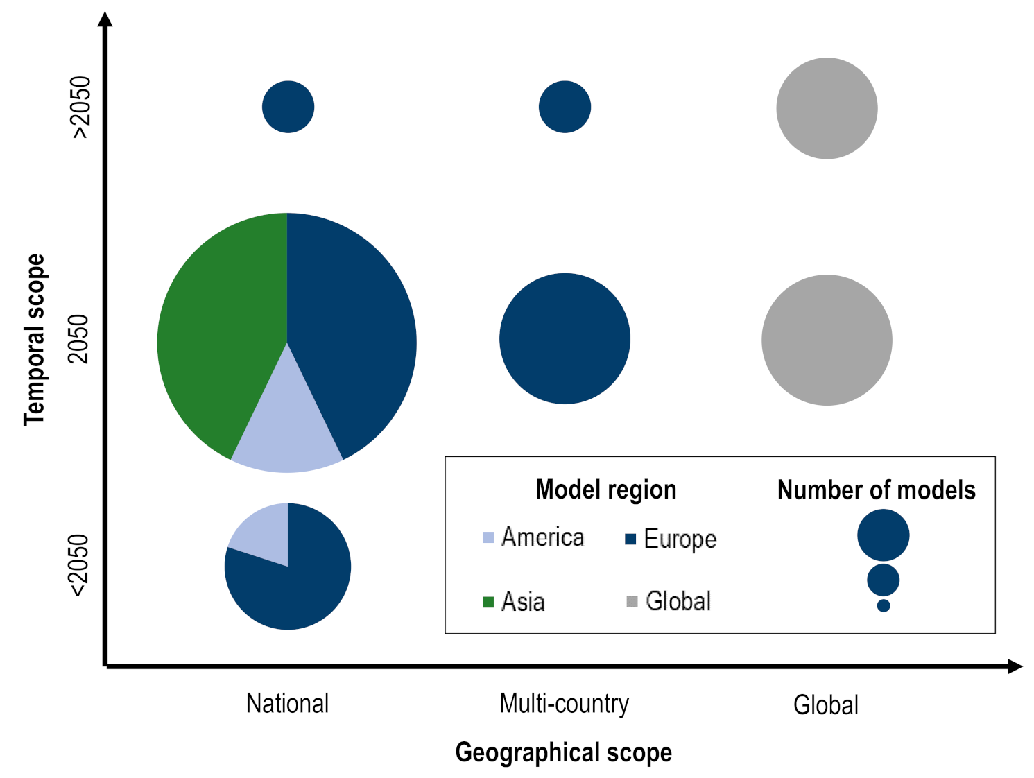
3. Boundary Conditions of Transport Sector Models
4. The Impact of Mobility Trends on the GHG Emission Calculation
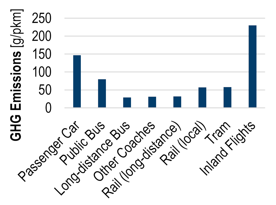
4.1. Modal Shift
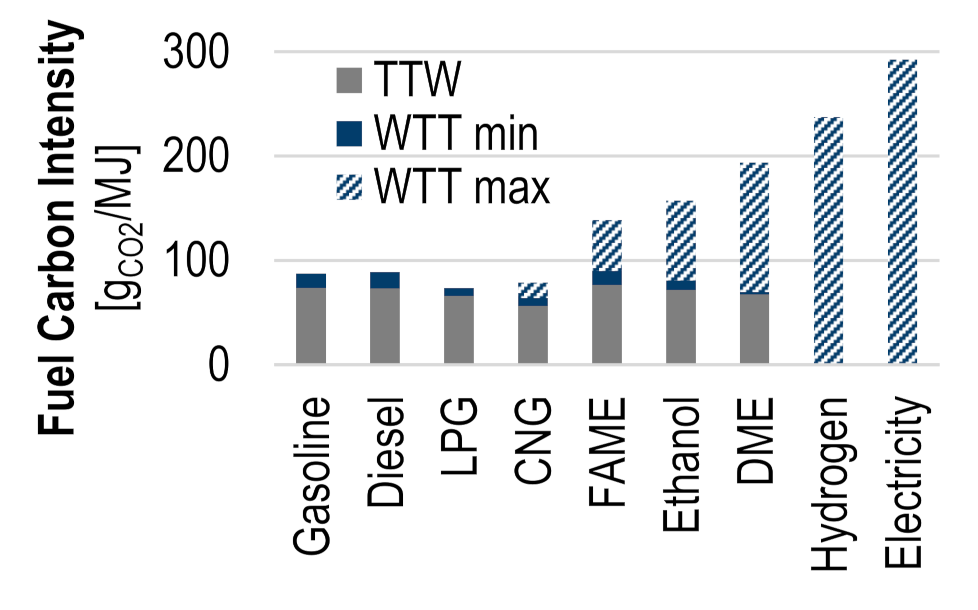
4.2. Fuel Shift
4.3. Shared Mobility
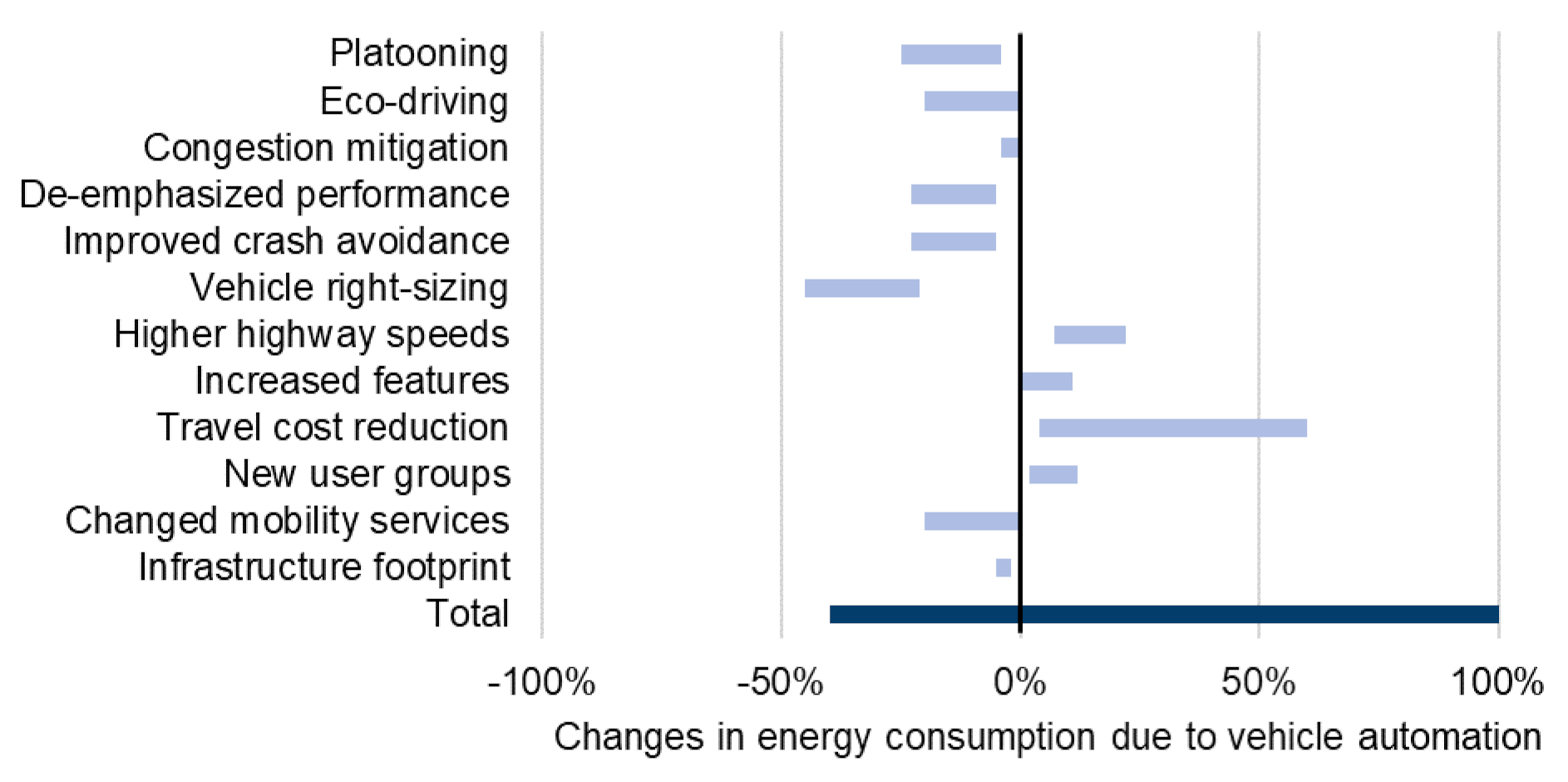
4.4. Automated Driving
5. Mobility Trends in Transport Sector Models
5.1. Modal Shift
5.2. Fuel Shift
5.3. Shared Mobility and Automated Driving
5.4. Comparison of Mobility Trends
6. Conclusions
Author Contributions
Funding
Institutional Review Board Statement
Informed Consent Statement
Conflicts of Interest
Appendix A. Model Information

| Model/Author | Ref | Spatial Scope | Temporal Scope | Spatial Resolution | Temporal Resolution | Sectoral Scope | ||||||||||||
|---|---|---|---|---|---|---|---|---|---|---|---|---|---|---|---|---|---|---|
| Region | National | Multi-country | Global | <2050 | −2050 | >2050 | <State Level | State Level | Country Level | >Country Level | <Hours | Hourly | Yearly | Passenger and Freight | Passenger Only | Freight Only | ||
| Renewbility III | [66] | Germany | x | x | x | x | x | |||||||||||
| ASTRA-DE | [68] | Germany | x | x | x | x | ||||||||||||
| VECTOR21 | [69] | Germany | x | x | x | x | x | |||||||||||
| VM-SIM | [70] | Germany | x | x | x | x | x | |||||||||||
| Shell | [64] | Germany | x | x | x | x | x | |||||||||||
| TraM | [71] | Germany | x | x | x | x | x | |||||||||||
| TEMPS | [65] | Germany | x | x | x | x | x | |||||||||||
| Trost | [50] | Germany | x | x | x | x | x | |||||||||||
| Belmonte et al. | [51] | Germany | x | x | x | x | x | |||||||||||
| SERAPIS | [72] | Austria | x | x | x | x | x | |||||||||||
| UKTCM | [73] | UK | x | x | x | x | x | |||||||||||
| STEAM | [74] | Scotland | x | x | x | x | x | |||||||||||
| DTReM-LV | [75] | Latvia | x | x | x | x | x | |||||||||||
| UniSyD | [76] | Iceland | x | x | x | x | x | |||||||||||
| Shepherd et al. | [77] | UK | x | x | x | x | x | |||||||||||
| TMOTEC | [45] | China | x | x | x | x | x | |||||||||||
| MA3T | [67] | US | x | x | x | x | x | |||||||||||
| ParaChoice | [61] | US | x | x | x | x | ||||||||||||
| ADOPT | [60] | US | x | x | x | x | x | |||||||||||
| CPREG | [78] | China | x | x | x | x | x | |||||||||||
| Hao et al. | [79] | China | x | x | x | x | x | |||||||||||
| LEAP | [80] | China | x | x | x | x | x | |||||||||||
| Palencia et al. | [81] | Japan | x | x | x | x | x | |||||||||||
| Gambhir et al. | [82] | China | x | x | x | x | x | |||||||||||
| Ou et al. | [83] | China | x | x | x | x | x | |||||||||||
| Yabe et al. | [54] | Japan | x | x | x | x | x | |||||||||||
| TRAN | [63] | US | x | x | x | x | x | |||||||||||
| PTTMAM | [58] | EU | x | x | x | x | ||||||||||||
| ASTRA-EC | [68] | EU | x | x | x | x | ||||||||||||
| TE3 | [20] | Germany, France, India, Japan, China, US | x | x | x | x | ||||||||||||
| HIGH-TOOL | [84] | EU | x | x | x | x | ||||||||||||
| PRIMES-TREMOVE | [85] | EU | x | x | x | x | ||||||||||||
| TRIMODE | [86] | EU | x | x | (x) | x | ||||||||||||
| TRAVEL | [44] | global | x | x | x | x | x | |||||||||||
| AIM/Transport | [46] | global | x | x | x | x | ||||||||||||
| MOVEET | [87] | global | x | x | (x) | x | ||||||||||||
| MoMo | [88] | global | x | x | (x) | x | ||||||||||||
| RoadMap | [41] | global | x | x | (x) | x | ||||||||||||
| ITEDD | [89] | global | x | x | (x) | x | ||||||||||||
| Khalili et al. | [90] | global | x | x | x | x | x | |||||||||||
| ForFITS | [91] | global | x | x | (x) | x | ||||||||||||
| Model/Author | Ref | Modes | Drivetrains | Energy Carriers | ||||||||||||||||||||
|---|---|---|---|---|---|---|---|---|---|---|---|---|---|---|---|---|---|---|---|---|---|---|---|---|
| Bicycle | Motorcycle | Car | LCV | HDV | Bus | Rail | Water | Air | ICEV | HEV | PHEV | REEV | BEV | FCEV | Gasoline | Diesel | Kerosene | CNG | Electricity | Hydrogen | Biofuels | Synthetic Fuels | ||
| Renewbility III | [66] | x | x | x | x | x | x | x | x | x | x | x | x | x | x | x | x | x | x | x | x | x | x | |
| ASTRA-DE | [68] | x | x | x | x | x | x | x | x | x | x | x | x | x | x | x | x | x | x | x | x | x | ||
| VECTOR21 | [69] | x | x | x | x | x | x | x | x | x | x | x | x | |||||||||||
| VM-SIM | [70] | x | x | x | x | x | x | x | x | x | x | x | x | |||||||||||
| Shell | [64] | x | x | x | x | x | x | x | x | x | x | x | x | x | ||||||||||
| TraM | [71] | x | x | x | x | x | x | x | x | x | x | x | x | x | x | x | x | x | x | x | ||||
| TEMPS | [65] | x | x | x | x | x | x | x | x | x | x | x | x | x | x | x | x | x | x | x | x | |||
| Trost | [50] | x | x | x | x | x | x | x | x | x | x | x | x | x | x | |||||||||
| Belmonte et al. | [51] | x | x | x | x | x | x | x | x | x | x | x | x | x | ||||||||||
| SERAPIS | [72] | x | x | x | x | x | x | x | x | x | ||||||||||||||
| UKTCM | [73] | x | x | x | x | x | x | x | x | x | x | x | x | x | x | x | x | x | x | x | x | x | ||
| STEAM | [74] | x | x | x | x | x | x | x | x | x | x | x | x | x | x | x | x | x | x | x | x | x | ||
| DTReM-LV | [75] | x | x | x | x | x | x | x | x | x | x | x | x | x | x | x | x | x | ||||||
| UniSyD | [76] | x | x | x | x | x | x | x | x | x | x | x | x | x | x | |||||||||
| Shepherd et al. | [77] | x | x | x | x | x | x | |||||||||||||||||
| TMOTEC | [45] | x | x | x | x | x | x | x | x | x | x | x | x | x | x | x | x | x | x | x | x | x | ||
| MA3T | [67] | x | x | x | x | x | x | x | x | x | x | x | x | x | ||||||||||
| ParaChoice | [61] | x | x | x | x | x | x | x | x | x | x | x | x | x | x | |||||||||
| ADOPT | [60] | x | x | x | x | x | x | x | x | x | x | x | x | x | ||||||||||
| CPREG | [78] | x | x | x | x | x | x | x | x | x | x | x | x | x | x | x | ||||||||
| Hao et al. | [79] | x | x | x | x | x | x | x | x | x | x | x | ||||||||||||
| LEAP | [80] | x | x | x | x | x | x | x | x | x | x | x | x | x | x | x | x | |||||||
| Palencia et al. | [81] | x | x | x | x | x | x | x | x | |||||||||||||||
| Gambhir et al. | [82] | x | x | x | x | x | x | x | x | x | x | x | x | x | x | x | x | |||||||
| Ou et al. | [83] | x | x | x | x | x | x | x | x | x | x | x | x | x | x | |||||||||
| Yabe et al. | [54] | x | x | x | x | x | x | x | ||||||||||||||||
| TRAN | [63] | x | x | x | x | x | x | x | x | x | x | x | x | x | x | x | x | x | x | x | ||||
| PTTMAM | [58] | x | x | x | x | x | x | x | x | x | x | x | x | x | ||||||||||
| ASTRA-EC | [68] | x | x | x | x | x | x | x | x | x | x | x | x | x | x | x | x | x | x | x | x | x | ||
| TE3 | [20] | x | x | x | x | x | x | x | x | x | x | x | x | |||||||||||
| HIGH-TOOL | [84] | x | x | x | x | x | x | x | x | x | x | x | x | x | x | x | x | x | x | x | x | x | x | |
| PRIMES-TREMOVE | [85] | x | x | x | x | x | x | x | x | x | x | x | x | x | x | x | x | x | x | x | ||||
| TRIMODE | [86] | x | x | x | x | x | x | x | x | x | x | x | x | x | x | x | x | x | x | x | x | x | x | |
| TRAVEL | [44] | x | x | x | x | x | x | x | x | x | x | x | x | x | x | x | x | x | x | x | ||||
| AIM/Transport | [46] | x | x | x | x | x | x | |||||||||||||||||
| MOVEET | [87] | x | x | x | x | x | x | x | ||||||||||||||||
| MoMo | [88] | x | x | x | x | x | x | x | x | x | x | x | x | x | x | x | x | x | x | x | x | x | ||
| RoadMap | [41] | x | x | x | x | x | x | x | x | x | x | x | x | (x) | x | x | x | x | x | x | x | |||
| ITEDD | [89] | x | x | x | x | x | x | x | x | |||||||||||||||
| Khalili et al. | [90] | x | x | x | x | x | x | x | x | x | x | x | x | x | x | x | x | x | x | x | x | |||
| ForFITS | [91] | x | x | x | x | x | x | x | x | x | x | x | x | x | x | x | x | x | x | x | x | x | x | |
| Model/Author | Ref | Mobility Trends | |||
|---|---|---|---|---|---|
| Modal Shift | Fuel Shift | Automated Driving | Sharing Mobility | ||
| Renewbility III | [66] | x | x | x | x |
| ASTRA-DE | [68] | x | x | x | |
| VECTOR21 | [69] | x | |||
| VM-SIM | [70] | x | |||
| Shell | [64] | x | x | ||
| TraM | [71] | x | |||
| TEMPS | [65] | x | x | x | x |
| Trost | [50] | x | |||
| Belmonte et al. | [51] | x | |||
| SERAPIS | [72] | x | |||
| UKTCM | [73] | x | x | ||
| STEAM | [74] | x | x | ||
| DTReM-LV | [75] | x | x | ||
| UniSyD | [76] | x | |||
| Shepherd et al. | [77] | x | |||
| TMOTEC | [45] | x | x | ||
| MA3T | [67] | x | x | x | |
| ParaChoice | [61] | x | |||
| ADOPT | [60] | x | |||
| CPREG | [78] | x | |||
| Hao et al. | [79] | x | |||
| LEAP | [80] | x | |||
| Palencia et al. | [81] | x | |||
| Gambhir et al. | [82] | x | |||
| Ou et al. | [83] | x | |||
| Yabe et al. | [54] | x | |||
| TRAN | [63] | x | |||
| PTTMAM | [58] | x | |||
| ASTRA-EC | [68] | x | x | x | |
| TE3 | [20] | x | |||
| HIGH-TOOL | [84] | x | x | ||
| PRIMES-TREMOVE | [85] | x | x | ||
| TRIMODE | [86] | x | x | ||
| TRAVEL | [44] | x | x | ||
| AIM/Transport | [46] | x | x | ||
| MOVEET | [87] | x | x | ||
| MoMo | [88] | x | x | ||
| RoadMap | [41] | x | x | ||
| ITEDD | [89] | x | x | ||
| Khalili et al. | [90] | x | x | ||
| ForFITS | [91] | x | x | ||
Appendix B. Boundary Conditions of Transport Sector Models
Appendix B.1. Spatio-Temporal Settings

Appendix B.2. Sectoral Coverage

Appendix C. Shared Mobility Concepts
- Car-sharing
- Personal vehicle sharing
- Ridesharing
- On-demand ride services
- Bike-sharing
Appendix D. Levels of Vehicle Automation
References
- Edelenbosch, O.Y.; McCollum, D.L.; van Vuuren, D.P.; Bertram, C.; Carrara, S.; Daly, H.; Fujimori, S.; Kitous, A.; Kyle, P.; Ó Broin, E.; et al. Decomposing passenger transport futures: Comparing results of global integrated assessment models. Transp. Res. Part D Transp. Environ. 2017, 55, 281–293. [Google Scholar] [CrossRef] [Green Version]
- Girod, B.; van Vuuren, D.P.; Grahn, M.; Kitous, A.; Kim, S.H.; Kyle, P. Climate impact of transportation A model comparison. Clim. Chang. 2013, 118, 595–608. [Google Scholar] [CrossRef] [Green Version]
- Yeh, S.; Mishra, G.S.; Fulton, L.; Kyle, P.; McCollum, D.L.; Miller, J.; Cazzola, P.; Teter, J. Detailed assessment of global transport-energy models’ structures and projections. Transp. Res. Part D Transp. Environ. 2017, 55, 294–309. [Google Scholar] [CrossRef] [Green Version]
- Linton, C.; Grant-Muller, S.; Gale, W.F. Approaches and Techniques for Modelling CO2Emissions from Road Transport. Transp. Rev. 2015, 35, 533–553. [Google Scholar] [CrossRef]
- Creutzig, F. Evolving Narratives of Low-Carbon Futures in Transportation. Transp. Rev. 2016, 36, 341–360. [Google Scholar] [CrossRef]
- Möller, T.; Padhi, A.; Pinner, D.; Tschiesner, A. The Future of Mobility is at Our Doorstep; McKinsey & Company: Cologne, Germany, 2019. [Google Scholar]
- Deloitte CASE Automotive Trends and Insights. Available online: https://www2.deloitte.com/us/en/pages/manufacturing/topics/case-automotive-industry.html (accessed on 30 July 2020).
- Toyota CASE. Available online: https://global.toyota/en/mobility/case/ (accessed on 30 July 2020).
- Daimler CASE–Intuitive Mobility. Available online: https://www.daimler.com/innovation/case-2.html (accessed on 30 July 2020).
- Litman, T. Autonomous Vehicle Implementation Predictions; Victoria Transport Policy Institute: Victoria, BC, Canada, 2020. [Google Scholar]
- LMC Automotive. The Outlook for Autonomous Vehicle Sales and Their Impact to 2050; LMC Automotive: Oxford, UK, 2018. [Google Scholar]
- Transport Systems Catapult. Market Forecast for Connected and Autonomous Vehicles; Transport Systems Catapult: Milton Keynes, UK, 2017. [Google Scholar]
- Schipper, L.; Marie-Lilliu, C. Transportation and CO2 Emissilons: Flexing the Link-A Path for the World Bank. In Environment Department Papers; International Energy Agency: Paris, France, 1999. [Google Scholar]
- PTV Austria GmbH. How does the City of Copenhagen Become the World’s Most Bike-Friendly City? PTV Austria GmbH: Vienna, Austria, 2019. [Google Scholar]
- Liu, R. The DRACULA Dynamic Network Microsimulation Model. In International Symposium on Transport Simulation; Springer: Boston, MA, USA, 2002. [Google Scholar]
- Joint Global Research Institute. Overview of the Global Change Assessment Model (GCAM); Pathways to Sustainable Energy Stakeholder Consultation Workshop: Bishkek, Kyrgystan, 2018. [Google Scholar]
- Stehfest, E.; van Vuuren, D.; Kram, T.; Bouwman, L.; Alkemade, R.; Bakkenes, M. Integrated Assessment of Global Environmental Change with IMAGE 3.0; PBL Netherlands Environmental Assessment Agency: The Hague, The Netherlands, 2014. [Google Scholar]
- Horni, A.; Nagel, K.; Axhausen, K.W. The Multi-Agent Transport Simulation MATSim; Ubiquity Press: London, UK, 2016. [Google Scholar]
- United Nations. Kyoto Protocol to the United Nations Framework Convention on Climate Change; United Nations: Kyoto, Japan, 1998. [Google Scholar]
- Jochem, P.; Möst, D. Model Description of TE3; KIT: Karslruhe, Germany; TU: Dresden, Germany, 2019. [Google Scholar]
- IEA Energy Intensity of Passenger Transport Modes. 2018. Available online: https://www.iea.org/data-and-statistics/charts/energy-intensity-of-passenger-transport-modes-2018 (accessed on 30 July 2020).
- Umwelt Bundesamt. Vergleich Der Durchschnittlichen Emissionen Einzelner Verkehrsmittel Im Personenverkehr in Deutschland-Bezugsjahr 2018; Umwelt Bundesamt: Dessau-Roßlau, Germany, 2020. [Google Scholar]
- IEA. Rail; IEA: Paris, France, 2020. [Google Scholar]
- Bilgin, B.; Magne, P.; Malysz, P.; Yang, Y.; Pantelic, V.; Preindl, M.; Korobkine, A.; Jiang, W.; Lawford, M.; Emadi, A. Making the Case for Electrified Transportation. IEEE Trans. Transp. Electrif. 2015, 1, 4–17. [Google Scholar] [CrossRef]
- Edwards, R.; Hass, H.; Larivé, J.-F.; Lonza, L.; Maas, H.; Rickeard, D. WELL-TO-WHEELS Report Version 4.a; JRC, EUCAR, CONCAWE: Luxembourg, 2014. [Google Scholar]
- Gaker, D.; Walker, J. Revealing the Value of “Green” and the Small Group with a Big Heart in Transportation Mode Choice. Sustainability 2013, 5, 2913–2927. [Google Scholar] [CrossRef] [Green Version]
- Machado, C.; de Salles Hue, N.; Berssaneti, F.; Quintanilha, J. An Overview of Shared Mobility. Sustainability 2018, 10, 4342. [Google Scholar] [CrossRef] [Green Version]
- Krueger, R.; Rashidi, T.H.; Rose, J.M. Preferences for shared autonomous vehicles. Transp. Res. Part C Emerg. Technol. 2016, 69, 343–355. [Google Scholar] [CrossRef]
- Kuhnert, F.; Stürmer, C.; Koster, A. Five Trends Transforming the Automotive Industry; PwC: Frankfurt am Main, Germany, 2018. [Google Scholar]
- Namazu, M.; MacKenzie, D.; Zerriffi, H.; Dowlatabadi, H. Is carsharing for everyone? Understanding the diffusion of carsharing services. Transp. Policy 2018, 63, 189–199. [Google Scholar] [CrossRef]
- Schäfer, A.W.; Yeh, S. A holistic analysis of passenger travel energy and greenhouse gas intensities. Nat. Sustain. 2020, 3, 459–462. [Google Scholar] [CrossRef]
- Martinez, L.M.; Correia, G.H.A.; Viegas, J.M. An agent-based simulation model to assess the impacts of introducing a shared-taxi system: An application to Lisbon (Portugal). J. Adv. Transp. 2015, 49, 475–495. [Google Scholar] [CrossRef]
- Jochem, P.; Babrowski, S.; Fichtner, W. Assessing CO2 emissions of electric vehicles in Germany in 2030. Transp. Res. Part A Policy Pract. 2015, 78, 68–83. [Google Scholar] [CrossRef] [Green Version]
- Wadud, Z.; MacKenzie, D.; Leiby, P. Help or hindrance? The travel, energy and carbon impacts of highly automated vehicles. Transp. Res. Part A Policy Pract. 2016, 86, 1–18. [Google Scholar] [CrossRef] [Green Version]
- Bösch, P.M.; Becker, F.; Becker, H.; Axhausen, K.W. Cost-based analysis of autonomous mobility services. Transp. Policy 2018, 64, 76–91. [Google Scholar] [CrossRef]
- Lammert, M.P.; Duran, A.; Diez, J.; Burton, K.; Nicholson, A. Effect of Platooning on Fuel Consumption of Class 8 Vehicles Over a Range of Speeds, Following Distances, and Mass. SAE Int. J. Commer. Veh. 2014, 7, 626–639. [Google Scholar] [CrossRef] [Green Version]
- Enzian, F.; Brzoska, I. Why Platooning is the Future of Delivery Traffic. Available online: https://www.mantruckandbus.com/en/innovation/why-platooning-is-the-future-of-delivery-traffic.html (accessed on 30 July 2020).
- Degraeuwe, B.; Beusen, B. Using on-board data logging devices to study the longer-term impact of an eco-driving course. Transp. Res. Part D Transp. Environ. 2013, 19, 48–49. [Google Scholar] [CrossRef]
- European Automobile Manufacturers Association New Passenger Car Registrations by Engine Capacity and Power. Available online: https://www.acea.be/statistics/article/new-passenger-car-characteristics-cubic-capacity-average-power (accessed on 30 June 2020).
- Baxter, J.A.; Merced Cirino, D.A.; Costinett, D.J.; Tolbert, L.M.; Ozpineci, B. Review of Electrical Architectures and Power Requirements for Automated Vehicles. In Proceedings of the IEEE Transportation Electrification Conference and Expo (ITEC), Long Beach, CA, USA, 13–15 June 2018. [Google Scholar]
- ICCT. ICCT Roadmap Model, Version 1-0; ICCT: Washington, DC, USA, 2012. [Google Scholar]
- Brand, C.; Tran, M.; Anable, J. The UK transport carbon model: An integrated life cycle approach to explore low carbon futures. Energy Policy 2012, 41, 107–124. [Google Scholar] [CrossRef] [Green Version]
- Ben-Akiva, M.; Lerman, S.R. Discrete Choice Analysis: Theory and Application to Travel Demand; The MIT Press: Cambridge, MA, USA, 1985. [Google Scholar]
- Girod, B.; van Vuuren, D.P.; Deetman, S. Global travel within the 2 °C climate target. Energy Policy 2012, 45, 152–166. [Google Scholar] [CrossRef] [Green Version]
- Wang, H.; Ou, X.; Zhang, X. Mode, technology, energy consumption, and resulting CO2 emissions in China’s transport sector up to 2050. Energy Policy 2017, 109, 719–733. [Google Scholar] [CrossRef]
- Mittal, S.; Dai, H.; Fujimori, S.; Hanaoka, T.; Zhang, R. Key factors influencing the global passenger transport dynamics using the AIM/transport model. Transp. Res. Part D Transp. Environ. 2017, 55, 373–388. [Google Scholar] [CrossRef]
- Hollevoet, J.; Witte, A.D.; Macharis, C. Improving insight in modal choice determinants: An approach towards more sustainable transport. In Urban Transport; WIT Press: Southampton, UK, 2011; Volume 116. [Google Scholar]
- Schäfer, A. Regularities in Travel Demand: An International Perspective. J. Transp. Stat. 2000, 3, 1–31. [Google Scholar]
- Siegemund, S.; Trommler, M.; Kolb, O.; Zinnecker, V. The Potential of Electricity-Based Fuels for Low-Emission Transport in the EU; Dena: Berlin, Germany, 2017. [Google Scholar]
- Trost, T. Erneuerbare Mobilität Im Motorisierten Individualverkehr; Forschungsgesellschaft für Straßen-und Verkehrswesen (FGSV): Leipzig, Germany; Stuttgart, Germany, 2017. [Google Scholar]
- Blat Belmonte, B.; Esser, A.; Weyand, S.; Franke, G.; Schebek, L.; Rinderknecht, S. Identification of the Optimal Passenger Car Vehicle Fleet Transition for Mitigating the Cumulative Life-Cycle Greenhouse Gas Emissions until 2050. Vehicles 2020, 2, 75–99. [Google Scholar] [CrossRef] [Green Version]
- Zimmer, W.; Blank, R.; Bergmann, T.; Mottschall, M.; Waldenfels, R. RENEWBILITY III-Die einzelnen RENEWBILITY-Modelle Im Detail; Ökoinstitut, DLR, IFEU, Infras: Berlin, Germany, 2015. [Google Scholar]
- Siskos, P.; Capros, P.; Zazias, G.; Fiorello, D.; Noekel, K. Energy and fleet modelling within the TRIMODE integrated transport model framework for Europe. Transp. Res. Procedia 2019, 37, 369–376. [Google Scholar] [CrossRef]
- Yabe, K.; Shinoda, Y.; Seki, T.; Tanaka, H.; Akisawa, A. Market penetration speed and effects on CO2 reduction of electric vehicles and plug-in hybrid electric vehicles in Japan. Energy Policy 2012, 45, 529–540. [Google Scholar] [CrossRef]
- Pichlmaier, S.; Fattler, S.; Bayer, C. Modelling the Transport Sector in the Context of a Dynamic Energy System. In Proceedings of the 41st IAEE International Conference, Groningen, The Netherlands, 10–13 June 2018. [Google Scholar]
- Lebeau, K.; Lebeau, P.; Macharis, C.; Van Mierlo, J. How expensive are electric vehicles? A total cost of ownership analysis. World Electr. Veh. J. 2013, 6, 996–1007. [Google Scholar] [CrossRef] [Green Version]
- Knupfer, S.M.; Hensley, R.; Hertzke, P.; Schaufuss, P. Electrifying Insights: How Automakers can Drive Electrified Vehicle Sales and Profitability; McKinsey & Company: Stamford, USA, 2017. [Google Scholar]
- Harrison, G.; Thiel, C.; Jones, L. Powertrain Technology Transition Market Agent Model (PTTMAM): An introduction; Joint Research Centre: Luxembourg, 2016. [Google Scholar]
- Struben, J.; Sterman, J.D. Transition Challenges for Alternative Fuel Vehicle and Transportation Systems. Environ. Plan. B Plan. Des. 2008, 35, 1070–1097. [Google Scholar] [CrossRef]
- Brooker, A.; Gonder, J.; Lopp, S.; Ward, J. ADOPT: A Historically Validated Light Duty Vehicle Consumer Choice Model. In Proceedings of the SAE 2015 World Congress and Exhibition, Detroit, MI, USA, 21–23 April 2015. [Google Scholar]
- Manley, D.; Levinson, R.; Barter, G.; West, T. ParaChoice-Parametric Vehicle Choice Modeling; Sandia National Lab: Albuquerque, NM, USA.
- Rogers, E. Diffusion of Innovations; Free Press: New York, NY, USA, 2003. [Google Scholar]
- U.S. Energy Information Administration. Transportation Sector Demand Module of the National Energy Modeling System: Model Documentation; U.S. Energy Information Administration: Washington, DC, USA, 2019.
- Adolf, J.; Balzer, C.; Joedicke, A.; Schabla, U.; Wilbrand, K.; Rommerskirchen, S.; Anders, N.; der Maur, A.a.; Ehrentraut, O.; Krämer, L.; et al. Shell PKW-Szenarien bis 2040; Shell, Prognos: Hamburg, Germany, 2014. [Google Scholar]
- Hacker, F.; Blanck, R.; Hülsmann, F.; Kasten, P.; Loreck, C.; Ludig, S.; Mottschall, M.; Zimmer, W. eMobil 2050-Szenarien Zum möglichen Beitrag Des elektrischen Verkehrs Zum Langfristigen Klimaschutz; Öko-Institut e.V.: Berlin, Germany, 2014. [Google Scholar]
- Zimmer, W.; Blank, R.; Bergmann, T.; Mottschall, M.; Waldenfels, R. Endbericht RENEWBILITY III-Optionen Einer Dekarbonisierung Des Verkehrssektors; Ökoinstitut, DLR, IFEU, Infras: Berlin, Germany, 2016. [Google Scholar]
- Xie, F.; Lin, Z. In Market Acceptance of Advanced Automotive Technologies–Mobility Choice (MA3T-MC): Consumer Acceptance of CAV, Shared Mobility and Electric Vehicle. In Proceedings of the Automated Vehicle Symposium 2019, Orlando, FL, USA, 16 July 2019. [Google Scholar]
- Fiorello, D.; Fermi, F.; Bielanska, D. The ASTRA model for strategic assessment of transport policies. Syst. Dyn. Rev. 2010, 26, 283–290. [Google Scholar] [CrossRef]
- Mock, P. Entwicklung eines Szenariomodells Zur Simulation Der Zukünftigen Marktanteile Und CO2-Emissionen Von Kraftfahrzeugen (VECTOR21); Universität Stuttgart: Stuttgart, Germany, 2010. [Google Scholar]
- Redelbach, M. Entwicklung Eines Dynamischen Nutzenbasierten Szenariomodells Zur Simulation Der Zukünftigen Marktentwicklung Für Alternative PKW-Antriebskonzepte; Deutsches Zentrum für Luft-und Raumfahrt: Stuttgart, Germany; Cologne, Germany, 2016. [Google Scholar]
- FfE. TraM-Sektormodell Des Verkehrs; FfE: Munich, Germany, 2017. [Google Scholar]
- Pfaffenbichler, P.; Renner, S.; Krutak, R. Modelling the Development of Vehicle Fleets with Alternative Propulsion Technologies; AEA: Vienna, Austria, 2011. [Google Scholar]
- Brand, C. UK Transport Carbon Model: Reference Guide; UK Energy Research Centre: Oxford, UK, 2010. [Google Scholar]
- Brand, C.; Cluzel, C.; Anable, J. Modeling the uptake of plug-in vehicles in a heterogeneous car market using a consumer segmentation approach. Transp. Res. Part A Policy Pract. 2017, 97, 121–136. [Google Scholar] [CrossRef]
- Barisa, A.; Rosa, M. A system dynamics model for CO2 emission mitigation policy design in road transport sector Aiga Barisa*, Marika Rosa. Energy Procedia 2018, 147, 419–427. [Google Scholar] [CrossRef]
- Shafiei, E.; Davidsdottir, B.; Leaver, J.; Stefansson, H.; Asgeirsson, E.I. Comparative analysis of hydrogen, biofuels and electricity transitional pathways to sustainable transport in a renewable-based energy system. Energy 2015, 83, 614–627. [Google Scholar] [CrossRef]
- Shepherd, S.; Bonsall, P.; Harrison, G. Factors affecting future demand for electric vehicles: A model based study. Transp. Policy 2012, 20, 62–74. [Google Scholar] [CrossRef]
- Peng, T.; Ou, X.; Yuan, Z.; Yan, X.; Zhang, X. Development and application of China provincial road transport energy demand and GHG emissions analysis model. Appl. Energy 2018, 222, 313–328. [Google Scholar] [CrossRef]
- Hao, H.; Liu, Z.; Zhao, F.; Li, W.; Hang, W. Scenario analysis of energy consumption and greenhouse gas emissions from China’s passenger vehicles. Energy 2015, 91, 151–159. [Google Scholar] [CrossRef]
- Liu, L.; Wang, K.; Wang, S.; Zhang, R.; Tang, X. Assessing energy consumption, CO2 and pollutant emissions and health benefits from China’s transport sector through 2050. Energy Policy 2018, 116, 382–396. [Google Scholar] [CrossRef]
- Palencia, J.C.G.; Otsuka, Y.; Araki, M.; Shiga, S. Impact of new vehicle market composition on the light-duty vehicle fleet CO2 emissions and cost. Energy Procedia 2017, 105, 3862–3867. [Google Scholar] [CrossRef]
- Gambhir, A.; Tse, L.K.C.; Tong, D.; Martinez-Botas, R. Reducing China’s road transport sector CO2 emissions to 2050: Technologies, costs and decomposition analysis. Appl. Energy 2015, 157, 905–917. [Google Scholar] [CrossRef] [Green Version]
- Ou, X.; Zhang, X.; Chang, S. Scenario analysis on alternative fuel/vehicle for China’s future road transport: Life-cycle energy demand and GHG emissions. Energy Policy 2010, 38, 3943–3956. [Google Scholar] [CrossRef]
- Szimba, E.; Ihrig, J.; Kraft, M.; Mitusch, K.; Chen, M.; Chahim, M.; van Meijeren, J.; Kiel, J.; Mandel, B.; Ulied, A.; et al. HIGH-TOOL–a strategic assessment tool for evaluating EU transport policies. J. Shipp. Trade 2018, 3, 11. [Google Scholar] [CrossRef]
- Karkatsoulis, P.; Siskos, P.; Paroussos, L.; Capros, P. Simulating deep CO2 emission reduction in transport in a general equilibrium framework: The GEM-E3T model. Transp. Res. Part D 2017, 55, 343–358. [Google Scholar] [CrossRef]
- Fiorello, D.; Nökel, K.; Martino, A. The TRIMODE integrated model for Europe. Transp. Res. Procedia 2018, 31, 88–98. [Google Scholar] [CrossRef]
- Purwanto, J.; de Ceuster, G.; Vanherle, K. Mobility, Vehicle fleet, Energy use and Emissions forecast Tool (MOVEET). Transp. Res. Procedia 2017, 25, 3421–3434. [Google Scholar] [CrossRef]
- Fulton, L.; Cazzola, P.; Cuenot, F. IEA Mobility Model (MoMo) and its use in the ETP 2008. Energy Policy 2009, 37, 3758–3768. [Google Scholar] [CrossRef]
- U.S. Energy Information Administration (EIA). Component Design Report: International Transportation Energy Demand Determinants Model; U.S. Energy Information Administration (EIA): Washington, DC, USA, 2017.
- Khalili, S.; Rantanen, E.; Bogdanov, D.; Breyer, C. Global Transportation Demand Development with Impacts on the Energy Demand and Greenhouse Gas Emissions in a Climate-Constrained World. Energies 2019, 12, 3870. [Google Scholar] [CrossRef] [Green Version]
- Cuenot, F. ForFITS at UNECE; iTEM4: Laxenburg, Austria, 2017. [Google Scholar]
- Weiss, M.; Dekker, P.; Moro, A.; Scholz, H.; Patel, M.K. On the electrification of road transportation-A review of the environmental, economic, and social performance of electric two-wheelers. Transp. Res. D Transp. Environ. 2015, 41, 348–366. [Google Scholar] [CrossRef] [PubMed]
- Greenblatt, J.B.; Shaheen, S. Automated Vehicles, On-Demand Mobility, and Environmental Impacts. Curr. Sustain./Renew. Energy Rep. 2015, 2, 74–81. [Google Scholar] [CrossRef] [Green Version]
- Atasoy, B.; Ikeda, T.; Ben-Akiva, M.E. Optimizing a Flexible Mobility on Demand System. Transp. Res. Rec. J. Transp. Res. Board 2019, 2563, 76–85. [Google Scholar] [CrossRef]
- SAE International. Levels of Driving Automation; J3016; SAE International: Warrendale, USA, 2014. [Google Scholar]
- Pearre, N.S.; Ribberink, H. Review of research on V2X technologies, strategies, and operations. Renew. Sustain. Energy Rev. 2019, 105, 61–70. [Google Scholar] [CrossRef]

| Modes | Drivetrains | Fuels |
|---|---|---|
| Bicycle | ICEV | Gasoline |
| Motorcycle | HEV | Diesel |
| Car | PHEV | Kerosene |
| LCV | REEV | CNG/LNG |
| HDV | BEV | Electricity |
| Bus | FCEV | Hydrogen |
| Rail | Biofuels | |
| Water | Synthetic fuels | |
| Air |
Publisher’s Note: MDPI stays neutral with regard to jurisdictional claims in published maps and institutional affiliations. |
© 2022 by the authors. Licensee MDPI, Basel, Switzerland. This article is an open access article distributed under the terms and conditions of the Creative Commons Attribution (CC BY) license (https://creativecommons.org/licenses/by/4.0/).
Share and Cite
Kraus, S.; Grube, T.; Stolten, D. Mobility Trends in Transport Sector Modeling. Future Transp. 2022, 2, 184-215. https://doi.org/10.3390/futuretransp2010010
Kraus S, Grube T, Stolten D. Mobility Trends in Transport Sector Modeling. Future Transportation. 2022; 2(1):184-215. https://doi.org/10.3390/futuretransp2010010
Chicago/Turabian StyleKraus, Stefan, Thomas Grube, and Detlef Stolten. 2022. "Mobility Trends in Transport Sector Modeling" Future Transportation 2, no. 1: 184-215. https://doi.org/10.3390/futuretransp2010010
APA StyleKraus, S., Grube, T., & Stolten, D. (2022). Mobility Trends in Transport Sector Modeling. Future Transportation, 2(1), 184-215. https://doi.org/10.3390/futuretransp2010010