Performance Evaluation of Multiple Pan-Sharpening Techniques on NDVI: A Statistical Framework

Abstract

Pan-sharpening is a pixel-level image fusion process whereby a lower-spatial-resolution multispectral image is merged with a higher-spatial-resolution panchromatic one. One of the drawbacks of this process is that it may introduce spectral or radiometric distortion. The degree to which distortion is introduced is dependent on the imaging sensor, the pan-sharpening algorithm employed, and the context of the scene analyzed. Studies that evaluate the quality of pan-sharpening algorithms often fail to account for changes in geographic context and are agnostic to any specific applications of an end user. This research proposes an evaluation framework to assess the effects of six widely used pan-sharpening algorithms on normalized difference vegetation index (NDVI) calculation in five contextually diverse geographic locations. Output image quality is assessed by comparing the empirical cumulative density function of NDVI values that are calculated by using pre-sharpened and sharpened imagery. The premise is that an effective algorithm will generate a sharpened multispectral image with a cumulative NDVI distribution that is similar to the pre-sharpened image. Research results revealed that, generally, the Gram–Schmidt algorithm introduces a significant degree of spectral distortion regardless of sensor and spatial context. In addition, higher-spatial-resolution imagery is more susceptible to spectral distortions upon pan-sharpening. Furthermore, variability in cumulative density of spectral information in fused images justifies the application of an analytical framework to assist users in selecting the most effective methods for their intended application.

1. Introduction

Panchromatic sharpening, known simply as pan-sharpening, is a broadly used radiometric transformation-based image fusion and enhancement technique that can merge a high-spatial-resolution panchromatic (PAN) image and a lower-spatial-resolution multispectral (MS) image to approximate a finer-spatial-resolution MS image (MSf) [1]. In other words, pan-sharpening can increase the spatial resolution of a MS image. Though most MS satellite images have a high spectral resolution, they often lack high spatial resolution because the input spectral signal received by the MS sensor is divided among multiple reflectance bands. PAN images, on the other hand, have high spatial resolution precisely because they integrate the energy of a wide spectral region, typically the visible to near-infrared region, to which silicon is sensitive, to allow for finer-spatial parsing of the available energy (i.e., electromagnetic waves). Pan-sharpening requires that input PAN and MS images be spatially co-registered, be in the same spatial reference system, be fully overlapped, have the same dimension (i.e., ground footprint), and have an assumption of identical scene conditions between the two image sets. It is most common, therefore, to merge PAN and MS images that are obtained coincidently from the same platform or even sensor (e.g., Landsat), such that the geometry and scene conditions are inherently identical.

Pan-sharpening is most frequently used to enhance the visual representation of a remotely sensed image. For example, most of the high-spatial-resolution images used in platforms such as Google Earth are created with pan-sharpening techniques [2]. These enhanced images allow users to distinguish and observe finer-scale features on the ground more reliably and accurately [3]. Pan-sharpening is designed to combine the high-spatial-resolution detail from PAN bands with the low-spatial-resolution but high-spectral-resolution detail from MS bands, creating an image which has not only high spatial resolution but also high spectral resolution [4]. Regardless of how well these conditions are satisfied, pan-sharpening inherently alters the values of multispectral bands, likely explaining its limited use as a preprocessing step for automated machine interpretation.

Over the past decades, researchers have developed a myriad of pan-sharpening algorithms that can be generally classified into one of three categories: (1) component substitution (CS), (2) multiresolution analysis (MRA), and (3) variational optimization (VO) [5]. A detailed description for each of these categories was provided in a study performed by Meng et al. [5], but a brief summary is given here. Mathematically, CS methods are the simplest, and they work by first conducting principal component analysis (PCA) on both the MS and PAN images and then normalizing the histograms of each by matching the spectral component from the MS image with the structural component from the PAN one to produce a single fused image with the principal spectral and structural information from both input images. MRA methods split the spatial information from the MS image and PAN image into two-band pass channels, known as approximations (i.e., low-frequency channel) and details (i.e., high-frequency channel). The high-frequency channels of the PAN image are injected into the corresponding interpolated MS bands at the same resolution as the PAN image, and, subsequently, the pan-sharpened MS data are reconstructed from the set of frequency bands [6]. VO methods approach pan-sharpening as an inverse optimization problem whereby a fused image is derived by generating an energy functional from the input MS and PAN images that is then passed into an optimization algorithm. In other words, VO methods focus on building the most effective and suitable models to characterize the correlation between the spectral information from the MS image with the spatial information in the PAN image [5,7,8,9]. A review of current industry-standard GIS software revealed that VO methods have yet to be widely adopted. Similarly, machine- and deep-learning approaches (see Reference [10]), which typically utilize a VO approach, are not readily available in industry-standard software packages.

The performance variability of each algorithm is determined largely by the geographic context of a given scene and the application orientation, or analytical goals at hand. This represents a significant gap in the extant pan-sharpening literature in that most pan-sharpening algorithm performance evaluation studies were focused mainly on one or a couple of geographic contexts [5]. As it stands, selecting the most effective pan-sharpening algorithm is an important decision, and performance evaluation is an essential step. In recent years, many studies have developed various metrics for performance evaluation, with most focused on examining the quality of the pan-sharpened image in terms of color preservation, spatial fidelity, and spectral fidelity [11,12,13,14,15,16,17,18]. However, because all pan-sharpening algorithms modify the pixel values of the original MS image, image products derived from the original MS image and pan-sharpened MS image can be expected to diverge. Index-specific performance evaluations, such as this evaluation on the calculation of normalized difference vegetation index (NDVI), hold promise to optimize pan-sharpening-algorithm selection for machine interpretation workflows which are dependent on deriving reliable indices. Thus, this research was focused on introducing a statistical framework (Figure 1) which can be used to assess the relative variability introduced in postprocessed pan-sharpened imagery and, ultimately, can be extensible to multiple application orientations, such as normalized difference water index (NDWI).

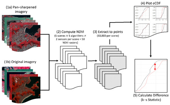
Figure 1. The workflow of the proposed statistical framework.

A review of the extant literature reveals that a framework for selecting among the myriad of widely adopted pan-sharpening algorithms in industry-standard software is lacking. The intellectual significance of this research lies in developing a framework for context-based pan-sharpening algorithm selection from a statistical perspective. Using one of the most common and frequently used spectral indices as a surrogate, the normalized difference vegetation index (NDVI), this research evaluated the performance of several pan-sharpening algorithms from a statistical perspective, or, more specifically, empirical cumulative distribution function (eCDF), which calculates the cumulative distribution of a sample’s empirical measure for a given variable value. This method is predicated on the assumption that differences in the overall spectral and radiometric information between an original and a fused image are the result of the pan-sharpening algorithm employed. The degree of spatial and spectral distortion introduced in a fused image can have significant impacts on the reliability of a derived index [19,20]. Thus, a comparison between the cumulative distribution of NDVI values in the original and fused images will allow us to quantify the degree of distortion introduced in the pan-sharpening process. The premise is that an ideal pan-sharpening algorithm will produce the same cumulative distribution of NDVI values of a given region from a MSf image as the original MS image. In other words, MSf NDVI’s empirical cumulative distribution pattern will be identical to that of NDVI calculated the original MS image.

2. Background

This study focused primarily on CS methods because they are the most widely employed and implemented in industry-standard GIS software; these include Brovey Transform (Brovey), Esri, Gram-Schmidt (GS), intensity-hue-saturation (IHS), and simple mean (SM) [21,22,23,24]. One MRA method based on wavelet transformations is supported in conventional GIS software and is also included [25,26,27]. No VO methods were analyzed in the present study, given the broad lack of implementation and adoption in conventional GIS software packages.

2.1. Pan-Sharpening Methods

In CS methods, a single component of the MS image, which is generally obtained by using a linear combination of the MS bands, is substituted with the PAN image. More precisely, the spatial information within the PAN image is extracted as the difference between the PAN image and the MS component and then injected back into the MS image, using a given injection scheme, such as the ones described below [5].

In Brovey image fusion, the multispectral image is resampled, and each pixel is multiplied by the ratio of the analogous PAN pixel intensity, and, subsequently, all MS pixel intensities are summed to generate the sharpened MS image [14]. Esri’s proprietary transformation algorithm applies a weighted average to the PAN image and adds the output adjustment value to each MS band [24]. Weighting factors can be multiplied by the ratio to create a pixel-by-pixel fused digital number, which is then multiplied by each band in the fused output image. The GS algorithm, which was patented in 2000 by Laben and Brower [22], works by first approximating a low-spatial-resolution image from the PAN input based on derived weights for each MS band. Next, each band combination is decorrelated by using GS decorrelation [28] to transform each band into a multidimensional vector with the number of dimensions equivalent to the number of pixels in the scene. Subsequently, the synthetic PAN band with coarser pixel size (PSc) is replaced with the original finer pixel size (PSf) one, and all bands are transformed to the PSf. In IHS transformations, the PSf PAN image replaces the intensity band of the low-spatial-resolution image and then converts the fused product back to an MS image with the same PSf. A weighting factor can be used to extract the spectral information of the near-infrared band [1,24]. SM image fusion algorithms calculate the simple mean of each MS band and the PAN band to extract the spatial structure information from the PAN image; the simple mean averaging equation is then applied to each of the PSf output MS bands.

WRM image fusion is an MRA method that decomposes the PAN image into three high-frequency features and one low-frequency feature by using a wavelet transformation. The low-frequency decomposition is then replaced with each low-spatial-resolution MS band and then reconstructed back into a fused MS image [5,29].

2.2. Pan-Sharpening for Vegetation Indices

Many spectral indices have been developed, but the most common and frequently used ones for Earth observation fall into a group known as vegetation indices (VIs). The prevalent method for obtaining high-spatial-resolution VIs is based on pan-sharpening [19,28,29,30]. It should be noted that the scope of the present study is not to propose new methods for calculating VIs; rather, we focus here on evaluating the performance of different pan-sharpening algorithms, using NDVI as a common surrogate for that analysis. Note also that, while the present study focuses on NDVI, we provide an extensible framework for other applications, including evaluating the variability of many indices in pan-sharpened images. Since the 1960s, remote-sensing scientists have estimated various biophysical characteristics of vegetation by using remotely sensed data. The vast majority of global biophysical monitoring and modeling efforts relies in VIs as inputs [1]. VIs have been used in many fields to improve the efficiency and quality of vegetation studies, including environmental and agricultural studies [1,31]. One of the most important indices is the NDVI, which correlates strongly with many measures of vegetation health [32] and is calculated by using only visible and near-infrared wavebands, which are collected by the vast majority of MS sensors.

NDVI is calculated as the normalized ratio between the visible red band and NIR band from an MS image:

$$\mathrm{NDVI}=\frac{\mathrm{NIR}-\mathrm{R}}{\mathrm{NIR}+\mathrm{R}}$$

(1)

where NIR denotes pixel values in the NIR band, while R denotes pixel values in the visible red band. Calculated NDVI values range from −1.0 to 1.0. Per Pettorelli [31] indicated the following:

Very low values of NDVI (≤0.1) correspond to barren areas of rock, sand, or snow. Free-standing water … tend[s] to be in the very low positive to negative values. Soils generally … tend to generate rather small positive NDVI values (roughly 0.1–0.2). Sparse vegetation such as shrubs and grasslands or senescing crops may result in moderate NDVI values (~0.2–0.5) High NDVI values (~0.6–0.9) correspond to dense vegetation.

(p. 32)

In instances where higher-spatial-MS-resolution imagery is cost-prohibitive or unavailable at the necessary temporal resolution, pan-sharpening is an attractive solution despite the apparent distortion of spectral information [33]. To wit, issues may arise in distinguishing spectral information at the boundaries of different land-use/land-cover types where pixel values are likely mixed [3]. While the loss of spectral information may be acceptable given the spatial, temporal, and analytical context, Johnson [3] found that most, if not all, of the spatial information injected into the MS image is also lost when a normalized VI such as the NDVI is derived from fused imagery by using the Brovey or smoothing filter-based intensity modulation (SFIM) algorithms. The same is true to a lesser extent with fast IHS, additive wavelet transform, and other methods reliant on multiplicative equations, because the influence of the PAN band is mathematically canceled out by the ratio employed in most Vis, including NDVI. According to the aforementioned process, the pan-sharpened NDVI (NDVI_ps) is calculated as follows:

$${\mathrm{NDVI}}_{\mathrm{ps}}=\frac{{\mathrm{NIR}}_{\mathrm{low}}\left(\mathsf{\delta }\right)-\mathrm{R}\left(\mathsf{\delta }\right)}{{\mathrm{NIR}}_{\mathrm{low}}\left(\mathsf{\delta }\right)+\mathrm{R}\left(\mathsf{\delta }\right)}$$

(2)

where $\mathsf{\delta }$ is the multiplicative function of a given algorithm, and low denotes the original low-spatial-resolution MS image. The multipliers on either side of the vinculum negate each other, leaving the original NDVI equation. However, because the output image is resampled to a smaller pixel size with potential spectral distortion, errors may compound and render an unreliable product. However, Rahaman et al. [34] argued that, if the NIR band is resampled prior to NDVI calculation, as is the case in the present study, the fused image is not mathematically canceled. Therefore, to get the NDVI values from a pan-sharpened image (NDVI_ps’), it should be calculated as follows:

$${\mathrm{NDVI}}_{{\mathrm{ps}}^{\prime }}=\frac{{\mathrm{NIR}}_{\mathrm{high}}-{\mathrm{R}}_{\mathrm{high}}}{{\mathrm{NIR}}_{\mathrm{high}}+{\mathrm{R}}_{\mathrm{high}}}$$

(3)

where high denotes the pan-sharpened high-spatial-resolution MS image. The diverging results reported in the studies conducted by Johnson [3] and Rahaman et al. [34] speak to growing concerns voiced within the pan-sharpening literature that systematic application-oriented reviews of multiple algorithms employ relatively few datasets and only focus on specific geographic regions, with little variation in terms of surficial and spectral features [5]. As such, the present study compared the outputs of multiple algorithms from multiple sensors across different geographic contexts.

3. Methods

3.1. Data Acquisition/Preprocessing

In total, ten pairs of MS and PAN images were acquired for this study. Geographically co-registered MS and PAN images were freely obtained from the US Geological Survey (USGS) and DigitalGlobe, covering spatially heterogeneous portions of San Francisco (US); Washington, D.C. (US); Tripoli (Libya); Stockholm (Sweden); and Rio de Janeiro (Brazil). These scenes are shown in Figure 2. Proprietary imagery from DigitalGlobe was collected by using the WorldView-4 satellite sensor, with the exception of San Francisco, for which imagery was collected by using QuickBird. The date of imagery acquisition is dependent on the availability of proprietary datasets. All Landsat scenes were selected to within two weeks of each proprietary scene to ensure temporal similarity between images. Only scenes with 0% cloud cover were analyzed to avoid further image processing operations to remove clouds. The spatial resolution of MS Landsat imagery is 30 m, MS WorldView-4 is 1.2 m, and MS QuickBird is 2.4 m. The spatial resolution of PAN Landsat imagery is 15 m, WorldView-4 imagery is 0.31 m, and QuickBird is 0.6 m. Where required, all imagery was reprojected to Universal Transverse Mercator (UTM).

Figure 2. Distribution and false-color composite representations of study areas: 1—Rio de Janeiro; 2—Washington, D.C.; 3—Tripoli; 4—San Francisco; 5—Stockholm. Acquisition dates are listed in Table 1.

Table 1. Summary of data sources.

Name	Source	PAN-GSD	MS-GSD	Bit Depth	Acquisition Date
Rio de Janeiro	WorldView-4	0.31 m	1.2 m	16-bit unsigned	27 September 2016
Rio de Janeiro	Landsat-8	15 m	30 m	16-bit unsigned	13 October 2016
Washington, D.C.	WorldView-4	0.31 m	1.2 m	16-bit unsigned	21 December 2019
Washington, D.C.	Landsat-8	15 m	30 m	16-bit unsigned	18 December 2019
Tripoli	WorldView-4	0.31 m	1.2 m	16-bit unsigned	21 December 2019
Tripoli	Landsat-8	15 m	30 m	16-bit unsigned	5 December 2019
San Francisco	QuickBird	0.6 m	2.4 m	8-bit unsigned	4 February 2016
San Francisco	Landsat-8	15 m	30 m	16-bit unsigned	20 February 2016
Stockholm	WorldView-4	0.31 m	1.2 m	16-bit unsigned	27 September 2016
Stockholm	Landsat-8	15 m	30 m	16-bit unsigned	12 September 2016

GSD = ground sampling distance.

Table 1. Summary of data sources.

Name	Source	PAN-GSD	MS-GSD	Bit Depth	Acquisition Date
Rio de Janeiro	WorldView-4	0.31 m	1.2 m	16-bit unsigned	27 September 2016
Rio de Janeiro	Landsat-8	15 m	30 m	16-bit unsigned	13 October 2016
Washington, D.C.	WorldView-4	0.31 m	1.2 m	16-bit unsigned	21 December 2019
Washington, D.C.	Landsat-8	15 m	30 m	16-bit unsigned	18 December 2019
Tripoli	WorldView-4	0.31 m	1.2 m	16-bit unsigned	21 December 2019
Tripoli	Landsat-8	15 m	30 m	16-bit unsigned	5 December 2019
San Francisco	QuickBird	0.6 m	2.4 m	8-bit unsigned	4 February 2016
San Francisco	Landsat-8	15 m	30 m	16-bit unsigned	20 February 2016
Stockholm	WorldView-4	0.31 m	1.2 m	16-bit unsigned	27 September 2016
Stockholm	Landsat-8	15 m	30 m	16-bit unsigned	12 September 2016

GSD = ground sampling distance.

3.2. Study Areas

The above sites were selected in an effort to represent a diversity of land-use and land-cover (LU/LC) contexts and because they were offered as free sample datasets through DigitalGlobe at the time of analysis. The extent of each of the five study sites was defined by the extent of the proprietary image. There is 100% overlap between each Landsat and the respective proprietary scene. In general, the scenes all represent randomly mixed LU/LC status. Figure 2 shows the global distribution of each study area and false-color composites (NIR, red, and green bands) of each. Washington, D.C., has the highest proportion of vegetative cover, and Tripoli has the lowest. The proportions of open water, built-up land, and barren land similarly vary across scenes. Table 2 lists approximate LU/LC statistics that were derived by using thematic rasters from the European Space Agency (ESA) GlobCover dataset (ESA 2009).

Table 2. Approximate percentage of GlobCover LU/LC classification types for each scene.

ESA GlobCover Classification	Washington, D.C.	Rio de Janeiro	Tripoli	Stockholm	San Francisco
Vegetation *	95%	57%	6%%	15%	25%
Artificial surfaces and associated areas	4.42%	13.82%	54%	78.04%	29.73%
Bare areas	0%	1.26%	23.76%	0	0
Water bodies	0.9%	26.25%	16.16%	6.97%	45.07%

* Vegetation is composite of the following ESA GlobCover classes: mosaic cropland (50–70%)/vegetation (grassland/shrubland/forest) (20–50%), mosaic vegetation (grassland/shrubland/forest) (50–70%)/cropland (20–50%), closed-to-open (>15%) broadleaved evergreen or semi-deciduous forest (>5 m), closed (>40%) broadleaved deciduous forest (>5 m), closed (>40%) needle-leaved evergreen forest (>5 m), open (15–40%) needle-leaved deciduous or evergreen forest (>5 m), closed-to-open (>15%) mixed broadleaved and needle-leaved forest (>5 m), mosaic forest or shrubland (50–70%)/grassland (20–50%), mosaic grassland (50–70%)/forest or shrubland (20–50%), closed-to-open (>15%) (broadleaved or needle-leaved; evergreen or deciduous) shrubland (<5 m), closed-to-open (>15%) herbaceous vegetation (grassland, savannas, or lichens/mosses), sparse (<15%) vegetation, closed-to-open (>15%) broadleaved forest regularly flooded (semi-permanently or temporarily).

Rio de Janeiro is a Brazilian megalopolis on the Western Atlantic Coast, where intensive infrastructural networks serve a consistently growing population. The built environment of Rio de Janeiro contrasts sharply with a precipitous topography, dense forests, and abundant freshwater bodies [35]. Washington, D.C., is a low-elevation urban core located in the Mid-Atlantic United States. The Potomac River converges with its tributary, the Anacostia River, at its southern borders with Virginia and Maryland. There are more than 7000 acres of parks within the District [36]. Tripoli is an ancient desert city on the Mediterranean coast of Northern Africa. Sparse vegetation contrasts with constructed water conveyances to support the large Libyan population [37]. San Francisco is the hilly urban center of the eponymous Bay Area situated between the Pacific Ocean to the west and San Francisco Bay to the east. Constructed parks dot the metropolitan core, and larger densely forested areas emerge at the metropolitan periphery [38]. Stockholm is an archipelago city located on Sweden’s east coast lowland near the Baltic Sea. Low-to-medium-density urban construction sits within large swaths of deciduous forest [39].

3.3. Image Pan-Sharpening

We created pan-sharpened images of each scene, using the Brovey, Esri, GS, IHS, SM, and WRM algorithms. All calculations were conducted in ArcMap (Version 10.7.1), with the exception of WRM, which was calculated by using ERDAS Imagine (Version 2015).

Prior to performing pan-sharpening via IHS, Brovey, Esri, and GS, optimal input band weight coefficients were calculated for each MS image, using the standard ArcGIS proprietary algorithm, which generates normalized weights based on the spectral sensitivity curves of each MS band. The MS band with the greatest overlap with the PAN band is weighted the highest, while any band with no overlap is weighted 0 [24]. The computed weights for each of the scenes are displayed in Table 3. Next, the pan-sharpening process was automated in a Python script, using the ArcPy library from Esri. Two separate scripts, one for the Landsat scenes and another for the proprietary scenes, are made publicly available in a GitHub repository (https://anonymous.4open.science/r/pansharpening-1BFE/README.md, accessed on 26 June 2022). WRM pan-sharpening was conducted manually on all ten scenes in ERDAS Imagine: for each scene, the spectral transformation was calculated by using PCA, and the pan-sharpened image was resampled by using nearest-neighbor interpolation. All pan-sharpened images were saved as 16-bit unsigned integer TIFF (.tif) raster datasets.

Table 3. Computed MS band weights used in the IHS, Brovey, Esri, and GS algorithms.

AOI	Landsat				Proprietary
	Red	Blue	Green	NIR	Red	Blue	Green	NIR
San Francisco	0.4023	0.5163	0.0814	0.0000	0.0356	0.4652	0.0000	0.4992
Rio de Janeiro	0.6317	0.0000	0.3408	0.2753	0.4834	0.0496	0.2857	0.1813
Stockholm	0.4930	0.3296	0.1687	0.0088	0.4041	0.1716	0.2195	0.2048
Tripoli	0.3894	0.5661	0.4447	0.0000	0.3937	0.0312	0.4153	0.1598
Washington, D.C.	0.5720	0.0000	0.4162	0.0118	0.3601	0.0941	0.3964	0.1494

All pan-sharpened scenes were compiled into one consolidated ArcMap document with individual data frames for each study site. We used Python to automate the calculation of NDVI from the pre-fused scenes and NDVI_ps’, using the R and NIR bands of each scene. Pixel values from all NDVI images were extracted to a matrix of 10,000 (100 × 100) equidistant points overlaid on each study area and then exported to five spreadsheets, which included 10,000 rows and 14 columns representing NDVI values calculated on both the pre- and post-sharpened Landsat and proprietary scenes.

3.4. eCDF Plotting

We calculated the eCDF of extracted NDVI values by using R statistical software (version 4.0.2). Figure 2 and Figure 3 show faceted plots comparing the eCDF of NDVI calculated, using pre-sharpened Landsat and proprietary scenery, respectively, with NDVI calculated after pan-sharpening for each algorithm included in this analysis. The eCDF is the distribution of an empirical measure of a sample—NDVI values, in this case—that increases by 1/n for each ordered data point in the set. The eCDF converges with the probabilistic cumulative distribution function (CDF) at 1, or 100% of the observations, where the probability of a variable, X, evaluated at x is less than or equal to X. Each NDVI value is sorted in ascending order and equals 0.01% of the entire distribution of observed points (1/10,000 × 100) for each NDVI (NDVI_j) calculation. Therefore, we have the following:

$${\widehat{\mathrm{eCDF}}}_{{\mathrm{NDVI}}_{\mathrm{j}}}\left({\mathrm{NDVI}}_{\mathrm{j}}\right)=\frac{10,000\le {\mathrm{NDVI}}_{\mathrm{j}}}{\mathrm{n}}=\frac{1}{\mathrm{n}}\sum _{\mathrm{i}=1}^{\mathrm{n}}{1}_{{\mathrm{X}}_{\mathrm{i}}}\le {\mathrm{NDVI}}_{\mathrm{j}}$$

(4)

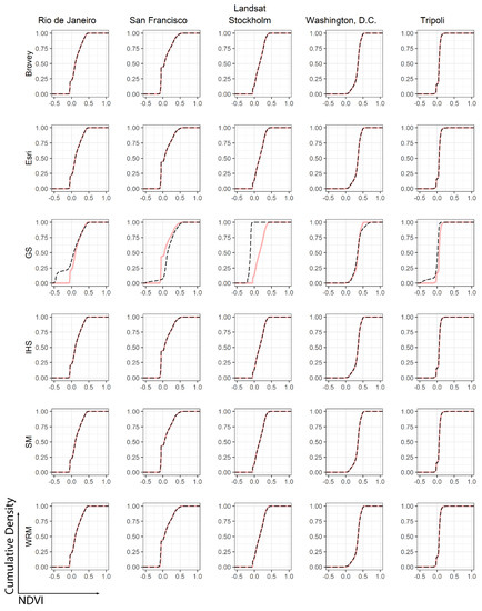
Figure 3. eCDF plots of NDVI calculated on pre-fused and pan-sharpened Landsat imagery. Pink line shows the eCDF of the original image’s NDVI, while black dashed line shows the eCDF of the pan-sharpened image’s NDVI.

The variance between the eCDF of NDVI calculated by using the pre-sharpened scenes and each algorithmic pan-sharpened one is understood to be caused by spectral and radiometric distortion or loss of fidelity from any given algorithm. In order to quantify this variance, we calculated a two-sample Kolmogorov–Smirnov (KS) statistic between NDVIs computed by using each pre-fused scene and each respective co-registered NDVI_ps’ image. The two-sample KS test (hereinafter referred to as KS) is a nonparametric statistical test that assesses whether two distributions are statistically equal. The KS statistic, D, represents the greatest distance on the y-axis between two eCDFs (or in a one-sample KS test, an eCDF and the probabilistic CDF curve). Because the KS test is nonparametric, it is necessary to first ensure that the distributions of the NDVI values for each scene are not normally distributed. As such, we first conducted the Shapiro–Wilk (SW) normality test on each NDVI set. In the SW test, the null hypothesis states that a given NDVI sample comes from a normal distribution. A p-value of substantially less than 0.01 will provide sufficient evidence to reject the null hypothesis to conclude that all NDVI sets are not normally distributed before proceeding to the KS test. The results of the SW normality tests are reported in Table 4.

Table 4. Results of the SW normality tests.

AOI	Algorithm	Landsat SW Statistic (W)	p-Value	Proprietary SW Statistic (W)	p-Value
Rio de Janeiro	Pre-fused	0.94287	<0.0001	0.92158	<0.0001
	Brovey	0.94326	<0.0001	0.92158	<0.0001
	Esri	0.94326	<0.0001	0.92158	<0.0001
	GS	0.92060	<0.0001	0.96281	<0.0001
	IHS	0.94326	<0.0001	0.92158	<0.0001
	SM	0.94326	<0.0001	0.92158	<0.0001
	WRM	0.94207	<0.0001	0.94638	<0.0001
San Francisco	Pre-fused	0.86692	<0.0001	0.86818	<0.0001
	Brovey	0.86764	<0.0001	0.98715	<0.0001
	Esri	0.86764	<0.0001	0.91479	<0.0001
	GS	0.87268	<0.0001	0.88993	<0.0001
	IHS	0.86764	<0.0001	0.96635	<0.0001
	SM	0.86764	<0.0001	0.92906	<0.0001
	WRM	0.87938	<0.0001	0.88751	<0.0001
Stockholm	Pre-fused	0.96186	<0.0001	0.94561	<0.0001
	Brovey	0.96111	<0.0001	0.94561	<0.0001
	Esri	0.96111	<0.0001	0.94561	<0.0001
	GS	0.93824	<0.0001	0.96344	<0.0001
	IHS	0.96111	<0.0001	0.94561	<0.0001
	SM	0.96111	<0.0001	0.94561	<0.0001
	WRM	0.84995	<0.0001	0.96727	<0.0001
Washington, D.C.	Pre-fused	0.93798	<0.0001	0.93798	<0.0001
	Brovey	0.93444	<0.0001	0.74406	<0.0001
	Esri	0.93444	<0.0001	0.77086	<0.0001
	GS	0.97589	<0.0001	0.92872	<0.0001
	IHS	0.93444	<0.0001	0.88188	<0.0001
	SM	0.93444	<0.0001	0.88431	<0.0001
	WRM	0.81412	<0.0001	0.85643	<0.0001
Tripoli	Pre-fused	0.94014	<0.0001	0.94014	<0.0001
	Brovey	0.93931	<0.0001	0.77817	<0.0001
	Esri	0.93931	<0.0001	0.77817	<0.0001
	GS	0.62166	<0.0001	0.94565	<0.0001
	IHS	0.93931	<0.0001	0.77817	<0.0001
	SM	0.93931	<0.0001	0.77817	<0.0001
	WRM	0.94425	<0.0001	0.75739	<0.0001

In this study, eCDF was used to calculate the cumulative distribution of a given x-value—in this case, NDVI. Subsequently, a probabilistic CDF can be used to determine the probability that a random observation that is taken from the population will be less than or equal to a certain value. Users can use this distribution pattern information to determine the probability that an observation will be greater than a certain value, or between two values of interest. The discrepancy between the baseline distribution and the post-distribution can be used to qualitatively assess the degree of variability. That being said, the discrepancy between the baseline distribution and the post-distribution can be used to assess how well the NDVI values extracted from the pan-sharpened image approximate the NDVI value extracted from the original MS image. The premise is that an effective algorithm will sharpen an image whose NDVI’s cumulative distribution pattern is similar or close to the original MS image.

The null hypothesis states that the extracted NDVI values from the original images and pan-sharpened images are normally distributed. The results revealed that all tested NDVI values have a p-value that is substantially less than 0.01 (Table 4); therefore, we reject the null hypothesis and conclude that there is sufficient evidence that the data tested are not normally distributed. Subsequently, the KS test was used to examine if, and the degree to which, the pan-sharpened NDVI eCDF distribution is statistically different from the original NDVI eCDF distribution for each scene. If the p-value of the KS test is statistically significant (i.e., <0.05), we conclude that the pre- and post-fused images are dissimilar, and that the given algorithm is thereby ineffective.

4. Results and Discussion

A total of 30 eCDF plots were created for Landsat and proprietary satellite images since there are five areas of interest (AOIs) and six pan-sharpening methods. As aforementioned, NDVI values range from −1.0 to 1.0; however, the x-axis values in these graphs only range from −0.5 to 1.0 to enhance visualization of the cumulative NDVI distributions where there is the most variance. It should be noted that the eCDF values (probability values) range from 0.0 to 1.0, and, therefore, the y-axis values in these graphs range from 0.0 to 1.0.

Interpreting Figure 4, we can see that all methods, except for GS, can be used to effectively pan-sharpen the entire collection of Landsat images (Rio de Janeiro; San Francisco; Stockholm; Washington, D.C.; and Tripoli) in the context of the NDVI, because the discrepancy between the baseline distribution and the post-distribution is visually minimal. The GS method cannot be used to effectively pan-sharpen any of the Landsat images. A further examination disclosed that the GS method involves an approximation process that could cause the discrepancy. To wit, the GS method approximates a low-spatial-resolution image from the high-spatial-resolution PAN image based on derived weights for each band. Weight selection is critical to the approximation process, and different band weights will create completely different low-spatial-resolution images. Currently, there are no well-established guidelines on how to select the weights for different satellite images, and most users use the software’s default weights for the approximation process. This could result in inappropriate weight selections for Landsat images, ultimately leading to the discrepancy between the baseline distribution pattern and the post-distribution pattern.

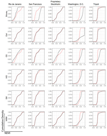
Figure 4. eCDF plots of NDVI calculated on pre-fused and pan-sharpened proprietary imagery. Pink line shows the eCDF of the original image’s NDVI, while black dashed line shows the eCDF of the pan-sharpened image’s NDVI.

Further exploration of the eCDF graphs reveals that the GS method has varying impacts on different Landsat images. The degree of variation is seemingly unassociated with the relative percentage of vegetation within each scene, but the eCDF curves tend to converge near the extreme low and high ends, where cumulative values are close to 0% and 100%, respectively. This is likely because GS decorrelation creates a vector of n dimensions based on the number of pixels in each band, thereby substantially increasing the potential sources of distortion.

There are no generalizable patterns between pre- and post-sharpened NDVI datasets derived from using proprietary imagery (Figure 4). That being said, the effective pan-sharpening methods vary for proprietary satellite images in the context of NDVI. For Rio de Janeiro, which is a Worldview-4 satellite image, the effective pan-sharpening methods are Esri, IHS, and SM in the context of NDVI, because the discrepancy between the baseline distribution and the post-distribution is visually minimal. Not surprisingly, both the Brovey and GS methods do not exhibit high performance, as a result of their computational complexity, as discussed above. The WRM method also shows some discrepancy. For San Francisco, none of the methods was effective in the context of NDVI; however, WRM may be effective because the discrepancy between the baseline distribution and the post-distribution is relatively small. Even so, further examination revealed that the discrepancy is large around the NDVI value of 0, potentially underestimating vegetation in built or barren areas. However, the Brovey, Esri, IHS, GS, and SM methods are not effective at all due to the large discrepancy. For Stockholm, the effective pan-sharpening methods are Brovey, Esri, IHS, and SM in the context of NDVI. However, the GS method and WRM method are not effective at all, due to the large discrepancy. For Washington, D.C., none of the pan-sharpening methods was effective in the context of NDVI since the discrepancy between the baseline distribution and the post-distribution is very large. That being said, when the Worldview-4 images for the Washington, D.C., area are used for pan-sharpening and subsequently used for NDVI analysis, Brovey, Esri, GS, IHS, SM, and WRM methods are not effective. Referring back to the GlobCover LU/LC distribution, we see that close to 95% of the Washington, D.C., scene consists of vegetation cover, followed by Rio de Janeiro (59%) and San Francisco (25%).

The results reveal that all tested NDVI eCDF distributions have varied results, which are summarized in Table 5. The KS statistic, D, is the absolute maximum distance between both eCDFs. For each pan-sharpened NDVI dataset, D statistics with an associated p-value less than 0.05 (95% confidence level) are statistically dissimilar from the pre-sharpened NDVI calculation, meaning that relatively smaller D values and corresponding p-values greater than 0.05 suggest that an algorithm is effective.

Table 5. Results of the two-sample Kolmogorov–Smirnov test.

AOI	Algorithm	Landsat KS Statistic (D)	Proprietary KS Statistic (D)
Rio de Janeiro	Brovey	0.0048	0.3641 **
	Esri	0.0048	0
	GS	0.2737 **	0.2592 **
	IHS	0.0048	0
	SM	0.0048	0
	WRM	0.0127	0.0396 **
San Francisco	Brovey	0.0035	0.7856 **
	Esri	0.0035	0.2604 **
	GS	0.4408 **	0.2227 **
	IHS	0.0035	0.1745 **
	SM	0.0035	0.1280 **
	WRM	0.1435 **	0.0381 **
Stockholm	Brovey	0.0069	0.0001
	Esri	0.0069	0.0001
	GS	0.9946 **	0.3246 **
	IHS	0.0069	0.0001
	SM	0.0069	0.0001
	WRM	0.0649 **	0.03834 **
Washington, D.C.	Brovey	0.0089	0.8819 **
	Esri	0.0089	0.6592 **
	GS	0.0885 **	0.5588 **
	IHS	0.0089	0.5014 **
	SM	0.0089	0.4584 **
	WRM	0.0241 **	0.5754 **
Tripoli	Brovey	0.0101	0.1967 **
	Esri	0.0101	0.1967 **
	GS	0.5828 **	0.7159 **
	IHS	0.0101	0.1967 **
	SM	0.0101	0.1967 **
	WRM	0.0357 **	0.1906 **

** Significant at p < 0.01.

To summarize, all methods, except for GS, can be used to effectively pan-sharpen the entire collection of Landsat images (Rio de Janeiro; San Francisco; Stockholm; Washington, D.C.; and Tripoli) in the context of NDVI, because the p-values are less than 0.01 (99% confidence interval). It is also noteworthy that, despite the visual similarity between the pre-sharpened NDVI dataset and the one derived from WRM in the eCDF plot, the KS test reveals small but statistically significant (p < 0.01) dissimilarities in all scenes but Rio de Janeiro. However, for proprietary satellite images, the KS test results closely resemble the visual analysis detailed above. For Rio de Janeiro, the effective methods in the context of NDVI are SM, IHS, and Esri, while the ineffective methods are WRM, GS, and Brovey. For Stockholm, the effective pan-sharpening methods are Brovey, Esri, IHS, and SM in the context of NDVI, while the GS method and WRM method are not effective. None of the tested methods was effective in the context of NDVI for San Francisco; Washington, D.C.; and Tripoli. However, the intention of the current study is not to make specific recommendations as to which pan-sharpening algorithm is most appropriate given the geographic context, because the ultimate objective of each practitioner may vary within the domain of interpreting VIs.

One possible explanation is that, the more a given scene is dominated by vegetation cover, the less accurate are the NDVI computations when derived from pan-sharpened imagery, with no extensible rule about which algorithm is superior or inferior. To test this, we assessed the relationship between the distribution of NDVI values and percentage of vegetation cover for each scene. Because the distribution of NDVI values for all scenes is not normally distributed, the difference between median NDVI values of the pre- and post-fused images is used to represent the variation introduced by each pan-sharpening algorithm. These differences and the percent vegetation cover present in each scene were transposed into the dataset displayed in Table 6.

Table 6. Percent vegetation cover and difference in median NDVI values for each scene and algorithm.

Scene/Sensor	% Veg. Cover	Difference in Median NDVI (Pre-Fused—Post-Fused)
		WRM	SM	IHS	GS	Brovey	Esri
Washington, D.C./Landsat	95%	−0.0015	−0.0010	−0.0010	0.0116	−0.0010	−0.0010
Washington, D.C./Proprietary	95%	−0.2652	−0.1263	−0.1540	−0.1951	−0.4117	−0.6471
Tripoli/Landsat	6%	−0.0003	−0.0003	−0.0003	0.0461	−0.0003	−0.0003
Tripoli/Proprietary	6%	0.0070	0.0069	0.0069	−0.2233	0.0069	0.0069
Stockholm/Landsat	15%	0.0002	−0.0004	−0.0004	0.2673	−0.0004	−0.0004
Stockholm/Proprietary	15%	−0.0280	0.0000	0.0000	0.2051	0.0000	0.0000
San Francisco/Landsat	25%	0.0052	0.0004	0.0004	−0.0029	0.0004	0.0004
San Francisco/Proprietary	25%	−0.0023	−0.0007	−0.0385	0.0140	−0.5385	0.0336
Rio de Janeiro/Landsat	57%	0.0000	0.0008	0.0008	0.0463	0.0008	0.0008
Rio de Janeiro/Proprietary	57%	−0.0039	0.0000	0.0000	0.0900	0.2046	0.0000

The SW normality test indicates that the distributions of percent vegetative cover and differences in median NDVI are not normally distributed. As such, the Spearman rank correlation coefficient was calculated between the percent vegetation cover and differenced median NDVI for each algorithm. The results, which are displayed in Table 7, indicate that, as vegetation cover increases, so too does the difference in median NDVI. The ρ values indicate a weak to moderate correlation (weak ρ = 0.1 = 0.3; moderate ρ = 0.3–0.5) that varies by the algorithm employed. Moreover, following the results of the KS test, this relationship is noticeably less pronounced when using the Brovey and GS algorithms, thus further suggesting an increased introduction of random distortion in the output PSf MS image. A simple linear regression between the percent of vegetation cover and difference in median NDVI shows that this relationship is significant (p = 0.002), with an R² of 0.2144. Model diagnostics suggest that the linear regression is acceptable—the residuals are normally distributed with only negligible evidence of kurtosis, and only one point (derived by using the Washington, D.C., proprietary image) is an outlier, but with little to no leverage. When the data points for the GS and Brovey algorithms are removed, the model significance increases somewhat, while the R² remains unchanged.

Table 7. Correlation between percent vegetation cover and difference in median NDVI values for each algorithm.

Algorithm	Correlation (ρ)	Degree
WRM	−0.492366	Moderate
SM	−0.4691716	Moderate
IHS	−0.4197851	Moderate
GS	−0.1477098	Weak
Brovey	−0.246183	Weak
Esri	−0.3703986	Moderate

These relatively low correlations and R² values are deemed acceptable, and they are even expected, in this context. First, the global land-cover classification is derived from the ESA GlobCover product, which has a spatial resolution of approximately 500 m. Second, the GlobCover product is an average LU/LC classification over time, while the scenes analyzed in the present study are at a single discrete moment. Finally, an ideal pan-sharpening algorithm is characterized by minimal distortion, which can stem from a vast array of potential sources of error or uncertainty. Vegetation cover, as it stands, can still reasonably account for 21.4% of the model variability in difference in median NDVI over and above the grand mean.

Additionally, the effect of differential bandwidth between MS and PAN bands cannot be overlooked. All three sensors that were analyzed in the present study have contrasting bandwidths between the MS and PAN bands, so it follows that spectral information is lost during the pan-sharpening process. Matsuoka et al. [40] conducted a sensitivity analysis exploring the effect of varying band position and bandwidth across multiple sensors on pan-sharpened images, finding that discrepancies in bandwidth do impart varying degrees. It is noteworthy that Matsuoka et al. identify a causal relationship between land-cover type and variability in fused image quality, specifically relating this variability to low contrast between vegetation and open water when employing the GS algorithm, regardless of sensor. This result is effectively replicated in the present analysis. To wit, GS is consistently outperformed by all other algorithms employed herein.

5. Conclusions

Pan-sharpening is an effective tool for increasing the visual interpretability of remotely sensed imagery in that it increases spatial resolution and provides a better visualization of a relatively low-spatial-resolution MS satellite image, using a single high-spatial-resolution PAN image. Moreover, pan-sharpening can improve the accuracy of image analysis, feature extraction, and modeling and classification [41]. The spatial and spectral context of a scene is often overlooked within the body of application-oriented pan-sharpening literature [5]. We highlighted one specific application in earth observation, NDVI, and systematically test the effects of multiple commercially available pan-sharpening algorithms on the calculation of NDVI. The assumption of the current study is that overall differences between the NDVI calculated from raw and pan-sharpened imagery is due to spectral or radiometric distortion, or loss of image fidelity, during the pan-sharpening process. The premise, therefore, is that an effective pan-sharpening algorithm will produce an image whose NDVI’s cumulative distribution pattern is similar or close to the original MS image.

We quantified the deviation introduced in the NDVI calculations after the pan-sharpening process and found that the deviation was increased by the spatial resolution of the input imagery and land-cover type—in this instance, the presence and abundance of vegetation. Similarly, error increases in geographic contexts with a higher degree of vegetative land cover. As such, we provide the following recommendations and procedure to assist users in selecting the most effective pan-sharpening algorithm for calculating the NDVI within their given context and application. First, avoid the GS and Brovey algorithms in favor of Esri, IHS, or SM for images with relatively coarse spatial resolution, such as Landsat, and exercise caution when selecting any pan-sharpening algorithm for imagery with a sub-meter ground sampling distance (GSD). Second, quantify the difference between the NDVI datasets calculated by using both the pre- and post-sharpened input imagery and select the algorithm that introduces the least distortion. Finally, the proposed analytical framework to quantitatively compare eCDF plots of the NDVI derived from using both pre- and post-fused imagery can assist with the qualitative identification of which algorithm introduces error and at which particular NDVI ranges of interest to the task at hand.

The framework proposed in the current study may also be extended to selecting the most effective pan-sharpening algorithms for different application contexts, such as soil or water indices. A limitation of the current framework is that the KS statistic represents the severity of difference between the eCDF functions being compared. It does not, however, quantify the overall extent or source of variance. Future research ought to focus on identifying the specific sources of distortion introduced by using any given pan-sharpening algorithm, the application of a sensitivity analysis to assess the effects of different band weights in pan-sharpening algorithms, and on the application of novel methods to the problem of pan-sharpening, which is outside the scope of the present study.

References

- Jensen, J.R. Remote Sensing of the Environment: An Earth Resource Perspective, 2nd ed.; Pearson: Upper Saddle River, NJ, USA, 2006. [Google Scholar]
- Kaur, G.; Saini, K.S.; Singh, D.; Kaur, M. A Comprehensive Study on Computational Pansharpening Techniques for Remote Sensing Images. Arch. Comput. Methods Eng. 2021, 28, 4961–4978. [Google Scholar] [CrossRef]
- Johnson, B. Effects of Pansharpening on Vegetation Indices. ISPRS Int. J. Geo-Inf. 2014, 3, 507. [Google Scholar] [CrossRef]
- Pushparaj, J.; Hedge, A.V. Comparison of Various Pan-Sharpening Methods using Quickbird-2 and Landsat-8 Imagery. Arabian J. Geosci. 2017, 10, 17. [Google Scholar] [CrossRef]
- Meng, X.; Shen, H.; Li, H.; Zhang, L.; Fu, R. Review of the Pansharpening Methods for Remote Sensing Images based on the Idea of Meta-Analysis: Practical Discussion and Challenges. Inf. Fusion 2019, 46, 102–113. [Google Scholar] [CrossRef]
- Hallabia, H.; Kallel, A.; Hamida, A.B. Image Pansharpening: Comparison of Methods based on Multiresolution Analysis and Component Substitution. In Proceedings of the 2014 1st International Conference on Advanced Technologies for Signal and Image Processing (ATSIP), Sousse, Tunisia, 17–19 March 2014; pp. 25–30. [Google Scholar] [CrossRef]
- Xie, Q.; Ma, C.; Guo, C.; John, V.; Mita, S.; Long, Q. Image Fusion Based on the Δ−1 − TV0 Energy Function. Entropy 2014, 16, 6099. [Google Scholar] [CrossRef]
- Liu, P.; Xiao, L.; Li, T. A Variational Pan-Sharpening Method Based on Spatial Fractional-Order Geometry and Spectral–Spatial Low-Rank Priors. IEEE Trans. Geosci. Remote Sens. 2018, 56, 1788–1802. [Google Scholar] [CrossRef]
- Tian, X.; Chen, Y.; Yang, C.; Ma, J. Variational Pansharpening by Exploiting Cartoon-Texture Similarities. IEEE Trans. Geosci. Remote Sens. 2022, 60, 1–16. [Google Scholar] [CrossRef]
- Zhang, H.; Xu, H.; Tian, X.; Jiang, J.; Ma, J. Image fusion meets deep learning: A survey and perspective. Inf. Fusion 2021, 76, 323–336. [Google Scholar] [CrossRef]
- Du, Q.; Gungor, O.; Shan, J. Performance Evaluation for Pan-Sharpening Techniques. Seoul 2005, 6, 4264–4266. [Google Scholar] [CrossRef]
- Du, Q.; Younan, N.H.; King, R.; Shah, V.P. On the Performance Evaluation of Pan-Sharpening Techniques. IEEE Geosci. Remote Sens. Lett. 2007, 4, 518–522. [Google Scholar] [CrossRef]
- Jawak, S.D.; Luis, A.J. A Comprehensive Evaluation of PAN-Sharpening Algorithms Coupled with Resampling Methods for Image Synthesis of Very High Resolution Remotely Sensed Satellite Data. Adv. Remote Sens. 2013, 2, 13. [Google Scholar] [CrossRef]
- Sarp, G. Spectral and Spatial Quality Analysis of Pan-sharpening Algorithms: A Case Study in Istanbul. Eur. J. Remote Sens. 2014, 47, 19–28. [Google Scholar] [CrossRef]
- Sunuprapto, H.; Danoedoro, P.; Ritohardoyo, S. Evaluation of Pan-sharpening Method: Applied to Artisanal Gold Mining Monitoring in Gunung Pani Forest Area. Procedia Environ. Sci. 2016, 33, 230–238. [Google Scholar] [CrossRef][Green Version]
- Kahraman, S.; Ertürk, A. A Comprehensive Review of Pansharpening Algorithms for Götürk-2 Satellite Images. In Proceedings of the ISPRS Annals of Photogrammetry, Remote Sensing and Spatial Information Sciences, Karabuk, Turkey, 14–15 October 2017; pp. 263–270. [Google Scholar] [CrossRef]
- Pushparaj, J.; Hedge, A.V. Evaluation of Pan-sharpening Methods for Spatial and Spectral Quality. Appl. Geomat. 2017, 9, 1–12. [Google Scholar] [CrossRef]
- Agudelo-Medina, O.A.; Benitez-Restrepo, H.D.; Vivone, G.; Bovik, A. Perceptual Quality Assessment of Pan-sharpened Images. Remote Sens. 2019, 11, 877. [Google Scholar] [CrossRef]
- Zhang, H.; Ma, J.; Chen, C.; Tian, X. NDVI-Net: A fusion network for generating high-resolution normalized difference vegetation index in remote sensing. ISPRS J. Photogramm. Remote Sens. 2020, 168, 182–196. [Google Scholar] [CrossRef]
- Tian, X.; Zhang, M.; Yang, C.; Ma, J. FusionNDVI: A Computational Fusion Approach for High-Resolution Normalized Difference Vegetation Index. IEEE Trans. Geosci. Remote Sens. 2021, 59, 5258–5271. [Google Scholar] [CrossRef]
- Haydan, R.; Dalke, G.W.; Henkel, J.; Bare, J.E. Applications of the IHS Colour Transform to the Processing of Multisensor Data and Image Enhancement. In Proceedings of the International Symposium on Remote Sensing of Arid and Semi-Arid Lands, Cairo, Egypt, 19–25 January 1982; pp. 599–626. [Google Scholar]
- Laben, C.A.; Brower, B.V. Process for Enhancing the Spatial Resolution of Multispectral Imagery Using Pan-Sharpening. U.S. Patent US6011875A, 2000. Available online: https://patents.google.com/patent/US6011875A/en (accessed on 28 January 2021).
- Maurer, T. How to Pan-Sharpen Images using the Gram-Schmidt Pan-Sharpen Method—A Recipe. Int. Arch. Photogramm. Remote Sens. Spat. Inf. Sci. 2013, XL-1/W1, 239–244. [Google Scholar] [CrossRef]
- Esri. Fundamentals of Panchromatic Sharpening. ArcGIS for Desktop. 2016. Available online: https://desktop.arcgis.com/en/arcmap/10.3/manage-data/raster-and-images/fundamentals-of-panchromatic-sharpening.htm (accessed on 24 June 2021).
- King, R.L.; Wang, J. A Wavelet based Algorithm for Pan Sharpening Landsat 7 Imagery. In Proceedings of the IGARSS 2001. Scanning the Present and Resolving the Future, Proceedings IEEE 2001 International Geoscience and Remote Sensing Symposium (Cat. No.01CH37217), Sydney, NSW, Australia, 9–13 July 2001; Volume 2, pp. 849–851. [Google Scholar] [CrossRef]
- Lemeshewsky, G.P. Multispectral Multisensor Image Fusion using Wavelet Transforms. In Proceedings of the Visual Information Processing VIII, Orlando, FL, USA, 5–9 April 1999; Volume 3716, pp. 214–222. [Google Scholar] [CrossRef]
- Lemeshewsky, G.P. Multispectral Image Sharpening using a Shift-invariant Wavelet Transform and Adaptive Processing of Multiresolution Edges. In Proceedings of the Visual Information Processing XI, Orlando, FL, USA, 1 April 2002; Volume 4736, pp. 189–200. [Google Scholar] [CrossRef]
- Aiazzi, B.; Baronti, S.; Selva, M.; Alparone, L. Bi-cubic interpolation for shift-free pan-sharpening. ISPRS J. Photogramm. Remote Sens. 2013, 86, 65–76. [Google Scholar] [CrossRef]
- Rahmani, S.; Strait, M.; Merkurjev, D.; Moeller, M.; Wittman, T. An Adaptive IHS Pan-Sharpening Method. IEEE Geosci. Remote Sens. Lett. 2010, 7, 746–750. [Google Scholar] [CrossRef]
- Wang, Q.; Shi, W.; Atkinson, P.M. Area-to-point regression kriging for pan-sharpening. ISPRS J. Photogramm. Remote Sens. 2016, 114, 151–165. [Google Scholar] [CrossRef]
- Pettorelli, N. The Normalized Difference Vegetation Index; Oxford University Press: Oxford, UK, 2013. [Google Scholar]
- Du, P.; Zhang, H.; Yuan, L.; Liu, P.; Zhang, H. Comparison of Vegetation Index from ASTER, CBERS and Landsat ETM+. In Proceedings of the 2007 IEEE International Geoscience and Remote Sensing Symposium, Barcelona, Spain, 23–28 July 2007; pp. 3341–3344. [Google Scholar] [CrossRef]
- Amro, I.; Mateos, J.; Vega, M.; Molina, R.; Katsaggelos, A.K. A Survey of Classical Methods and New Trends in Pansharpening of Multispectral Images. EURASIP J. Adv. Signal Process. 2011, 2011, 79. [Google Scholar] [CrossRef]
- Rahaman, K.R.; Hassan, Q.K.; Ahmed, M.R. Pan-sharpening of Landsat-8 Images and Its Application in Calculating Vegetation Greenness and Canopy Water Contents. ISPRS Int. J. Geo-Inf. 2017, 6, 168. [Google Scholar] [CrossRef]
- Godfrey, B.J. Revisiting Rio De Janeiro and são Paulo. Geogr. Rev. 1999, 89, 94–121. [Google Scholar] [CrossRef]
- Interstate Commission on the Potomac River Basin. General Facts & FAQs. 2012. Available online: http://www.potomacriver.org/2012/facts-a-faqs/faqs (accessed on 25 May 2022).
- Rghei, A.S.; Nelson, J.G. The Conservation and Use of the Walled City of Tripoli. Geogr. J. 1994, 160, 143–158. [Google Scholar] [CrossRef]
- Scott, M. The San Francisco Bay Area: A Metropolis in Perspective; University of California Press: Berkeley, CA, USA, 1985. [Google Scholar]
- Hobbs, J.J. World Regional Geography; Cengage Learning: Boston, MA, USA, 2008. [Google Scholar]
- Matsuoka, M.; Tadono, T.; Yoshioka, H. Effects of the spectral properties of a panchromatic image on pan-sharpening simulated using hyperspectral data. Int. J. Image Data Fusion 2016, 7, 339–359. [Google Scholar] [CrossRef]
- Yang, S.; Wang, M.; Jiao, L. Fusion of Multispectral and Panchromatic Images based on Support Value Transform and Adaptive Principal Component Analysis. Inf. Fusion 2012, 13, 177–184. [Google Scholar] [CrossRef]
Publisher’s Note: MDPI stays neutral with regard to jurisdictional claims in published maps and institutional affiliations. |
© 2022 by the authors. Licensee MDPI, Basel, Switzerland. This article is an open access article distributed under the terms and conditions of the Creative Commons Attribution (CC BY) license (https://creativecommons.org/licenses/by/4.0/).