Article

Amplification in Time and Dilution in Space: Partitioning Spatiotemporal Processes to Assess the Role of Avian-Host Phylodiversity in Shaping Eastern Equine Encephalitis Virus Distribution

by
John M. Humphreys
Pest Management Research Unit, Agricultural Research Service, US Department of Agriculture, 1500 N. Central Avenue, Sidney, MT 59270, USA
Geographies 2022, 2(3), 419-434; https://doi.org/10.3390/geographies2030026
Submission received: 26 May 2022 / Revised: 5 July 2022 / Accepted: 6 July 2022 / Published: 8 July 2022
(This article belongs to the Special Issue Feature Papers of Geographies in 2022)

Abstract

:
Eastern equine encephalitis virus (EEEv) is an arthropod-borne virus and the causative agent of neurologic disease in humans, horses, poultry, and wildlife. Although EEEv is known to be transmitted in cycles involving avian hosts and ornithophilic mosquitoes, there is ongoing debate about the role avian-host phylodiversity plays in diluting or amplifying virus prevalence across geographic space and through time. This study leveraged seventeen years of non-human EEEv detections to quantify possible EEEv dilution and amplification effects in response to avian-host phylodiversity. In assessing EEEv and avian-host diversity relationships, comparisons were performed to illustrate how modeling decisions aimed at capturing spatial patterns, temporal trends, and space–time interactions impacted results and the interpretations drawn from those results. Principal findings indicated that increased avian phylodiversity promotes EEEv dilution across geographic space, but this dilution effect is scale-dependent and masked by amplification effects that occur through time. Findings further demonstrated that the decisions made when modeling complex spatiotemporal dynamics can readily contribute to contrasting statistical outcomes and results misinterpretation, even when arithmetic and mathematics are strictly correct.

1. Introduction

Eastern equine encephalitis virus (EEEv) is an arthropod-borne virus (arbovirus) and the causative agent of eastern equine encephalitis (EEE) disease in humans, horses, poultry, and wildlife [1,2,3]. EEEv infection in livestock occurs more frequently than in humans, with horses being particularly vulnerable to disease. Between 2006 and 2020, the eastern United States (US) averaged more than 150 horse EEE cases annually, with infected horses exhibiting symptoms that ranged from fever and impaired vision to paralysis, convulsions, and death [4]. Although more rare, human mortality resulting from EEE disease can be as high as 30% and persons with the disease may exhibit long-term neurologic ailment [5]. Human EEE incidence is closely associated with horse outbreaks and recent evidence suggests that the geographic range of EEEv may be expanding further north and contributing to increased virus infection rates in both humans and horses [1,6]. Because EEEv poses a growing challenge to livestock and public health, research describing EEEv spatiotemporal distribution is needed to improve disease surveillance and better anticipate future outbreaks.
EEEv is transmitted in cycles involving avian hosts and ornithophilic mosquitoes, with birds in the Order Passeriformes serving as principal virus reservoirs in the transmission process [2,7,8,9]. Humans, horses, and other mammals exhibit a low viremic response to infection and are, therefore, considered incidental or “dead end” hosts in the EEEv cycle [10,11,12,13]. Unlike other bird-mediated zoonotic viruses, such as avian influenza [14,15,16], environmental contamination is not recognized as a major component of EEEv transmission; thus, the EEEv ecological niche is better described by passerine occurrence and community composition than it is by the ambient climate or environmental conditions external to birds. Given their obligate role in virus transmission, passerine hosts are key to understanding EEEv distribution and prevalence at the landscape scale.
Passerines are the largest and most diverse group of birds in the US and exhibit movement behavior that ranges from local dispersal to transcontinental migration, frustrating attempts at selecting any single species as an archetypal arbovirus reservoir [17,18]. Because individual bird species are nested in ecological communities where they interact with other hosts and non-hosts (i.e., disease contact processes), migration and dispersal serve to further complicate analysis, as bird movement bridges local communities with those at distance, thus, shaping virus prevalence at the local scale and transmission at the landscape scale [18,19,20]. Stated differently, transiting birds physically transport EEEv between different localities while simultaneously shifting host-community composition and diversity at both the departure and arrival sites. As host composition and diversity change at a location, so too does the total number of vector-hosts contacts, the proportion of those contacts that link vectors with competent avian species, and overall virus prevalence [21,22].
The generality of host phylodiversity and pathogen interactions across different disease systems and spatial-temporal scales is an active topic for debate in ecology [23,24,25,26]. Diversity–pathogen relationships have been variably argued as exhibiting a “dilution effect,“ in which increased diversity reduces prevalence, transmission rates, and disease risk [27,28], or as showing an “amplification effect” by which increased diversity contributes to elevated pathogen numbers [21,29]. Empirical and experimental evidence has been advanced in support of both dilution and amplification effects in a wide variety of disease systems [25,26]; however, missing from the debate is discussion of how dilution or amplification effects are statistically identified, quantified, and reported.
Modeling approaches that evaluate complex disease systems as snapshots in time or place are insufficient to infer epidemiologic processes that occur dynamically [30]. As described by Abellan et al. [31], static models that consider the spatial dimension in the absence of temporal change may provide some limited insight into disease risk factors that are stationary or constant; however, such methods are inadequate for determining short-term, time-variable, or emergent risks. In the EEEv system, pathogen prevalence varies both spatially and temporally as avian hosts move throughout their territorial range or relocate viruses as part of annual migration. To assess disease prevalence, it is necessary to explicitly model these spatial and temporal trends, as well as any correlations or interactions that may exist between them [32]. The decisions researchers make when selecting methods or modeling techniques have major implications for what results are produced and how those results are ultimately interpreted [33,34]. Although there can be endless debate about what goes into a model and how model results are interpreted, it is clear that analyses that leverage spatially and temporally structured data to quantify complex ecological dynamics without careful consideration of model spatiotemporal covariates are prone to misinterpretation, even when arithmetic and mathematics are strictly correct.
The current study has two major objectives. First, because EEEv poses a growing challenge to livestock and public health across the entirety of the eastern US, seventeen years of non-human EEEv detections are applied to quantify the correspondence of virus prevalence to passerine-host phylodiversity. The second study objective is to assess how the modeling of spatial patterns, temporal trends, and space–time interactions under different statistical implementations changes results and how those results are interpreted with respect to possible dilution and amplification effects in the EEEv system.

2. Materials and Methods

2.1. Study Domain and Virus Data

The study domain for analysis included the twenty-six US states located east of the Mississippi River, plus the geographically contiguous states of Louisiana and Arkansas found immediately west of the Mississippi River. This study domain exhibited a total areal extent of approximately 2.5 million km 2 and was inclusive of 1746 county-level jurisdictional units that defined the minimum spatial resolution for analysis. Counties were chosen as the resolution for modeling due to virus detection data being available at the county level. Study observation data were obtained from the Centers for Disease Control and Prevention (CDC) [35] and consisted of all non-human EEEv detections documented during the seventeen year period 2003–2019. Virus detection data included attributes reflecting the count of confirmed EEEv detections reported within each county, the host species from which the virus was collected, and the date of virus collection. For the current study, virus-collection dates were aggregated to weekly time steps. Annual counts of EEEv detection are shown in Figure 1 and are color coded to distinguish samples collected from mosquito, mammal (primarily Equidae), sentinel chicken, or wild-bird hosts. ArboNET is a passive surveillance system. It is dependent on clinicians considering the diagnosis of an arboviral disease and obtaining the appropriate diagnostic test, and reporting of laboratory-confirmed cases to public health authorities. Diagnosis and reporting are incomplete, and the incidence of arboviral diseases is underestimated.

2.2. Climate Data

Daily total precipitation and maximum temperature grids (4 km 2 resolution) for the US (2003–2019) were acquired from the PRISM Climate Group [36] and averaged (temperature) or summed (precipitation) to weekly increments to correspond with week-based EEEv observations. Weekly temperature and precipitation grids were then averaged to the county level, to match the spatial resolution of EEEv detections.

2.3. Avian-Host Occurrence and Phylodiversity

Avian occurrences recorded in the Cornell Lab of Ornithology eBird database [37] were spatially filtered to study area boundaries and then cross-referenced with those species included in the Global Phylogeny of Birds [38] (https://birdtree.org/, accessed on 5 July 2022) to identify the passerines (Order Passeriformes) found in both the study domain and global phylogeny. Passerine locations and observation dates were next matched to EEEv detection data to identify each species’ presence or absence within each county during each week of the year. To help reduce rare species numbers, a minimum of two species-specific bird observations were required to qualify as a presence for a given county and week. The resulting avian-community matrices were used to calculate total species richness by county and week, as well as to index interspecies branch lengths from the phylogeny to estimate phylodiversity.
Avian phylodiversity was estimated by trimming the time−calibrated global phylogeny to the study-domain species pool (207 species) before sampling this subset from a pseudo−posterior distribution [38]. Bootstrap replicate trees (1000) were then summarized as a maximum clade credibility tree using TreeAnnotator (http://beast.community/treeannotator, accessed on 5 July 2022) and the BEAST 2 package [39].
Avian-host phylodiversity (PD) was calculated using the consensus tree and avian-community matrices. To judge statistical importance and departures from species-pool averages, PD estimates were compared to a null model derived from 999 consensus-tree random permutations using the picante package [40].

2.4. Statistical Analysis

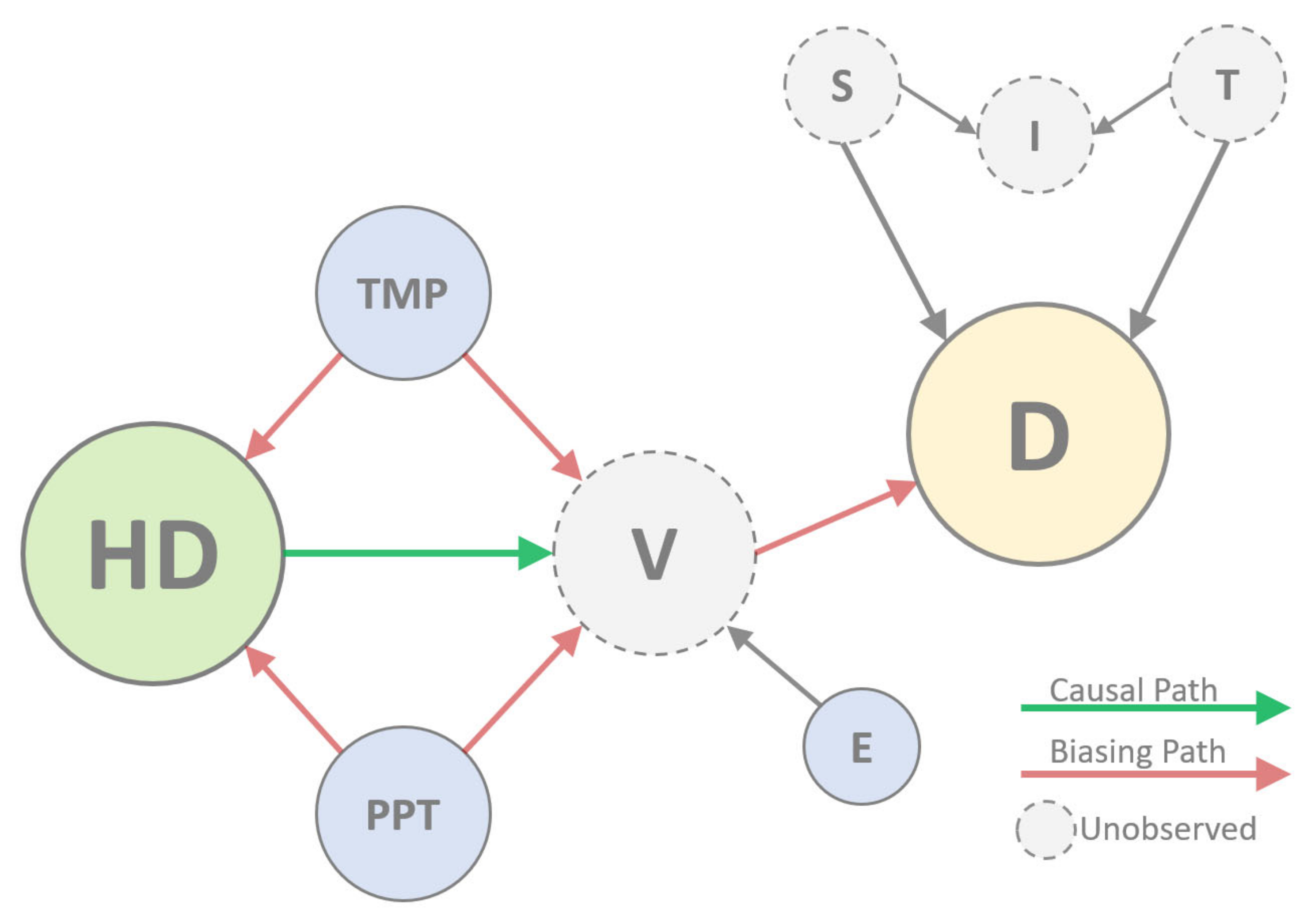
Bayesian spatiotemporal models were adopted to evaluate the relationship between EEEv detections and avian-host phylodiversity. A central objective of analysis was to assess how different implementations of spatial, temporal, and space–time interaction effects altered results and ultimately changed how those results were interpreted with respect to possible dilution effects. Drawing from a causal analysis perspective, the directed acyclic graph (DAG) shown in Figure 2 summarizes principal assumptions and hypotheses underlying statistical-model development. Although causal inference is often misunderstood as a procedure only applied to experimental or clinical research, it is appropriate for evaluation of observational data used in ecological and epidemiological studies [41,42,43,44].
As illustrated in the graphical heuristic (Figure 2), avian-host diversity (HD) is hypothesized to exhibit a causal relationship to “true” virus prevalence (V) in the environment. This hypothesis is illustrated by an arrow from HD (the cause) to V (the effect). Because true or actual prevalence is unobserved and unknown, reported virus detections (D) are used to approximate actual prevalence with concurrent estimation of unobserved error arising from spatial (S), temporal (T), and space–time interactions (I). Estimation of S, T, and I effects are the focus of this study. Although prevalence is assumed to be a function of avian-host diversity, it is also hypothesized that average exposure (E) rates and “common cause” confounds such as temperature (TMP) and precipitation (PPT) intercede in the causal chain to bias effect estimation. Given the potential for climate-linked confounds, models were also adjusted for TMP and PPT.
Although several different statistical formulations were compared to evaluate S, T, and I effects, the general template for all models was of the form,
Y s t Poisson ( λ st )
λ s t = E s t ρ s t
l o g ( ρ s t ) = η s t
η s t = α + β x X s t + u s + υ s + γ t + ϕ t + δ s t ,
where the number of EEEv detections ( Y s t ) in county s ( s = 1 , 2 , 3 , , 1746 ) during week t ( t = 1 , 2 , 3 , , 52 ) followed a Poisson distribution with a mean λ s t (Equation (1)). When modeling disease case counts, the mean rate can be estimated as the product of the expected case number E s t (calculated from standardized incidence and population size) and the disease rate or relative risk ρ s t . However, because the current study assessed virus counts rather than disease cases, E s t was instead interpreted as an environmental exposure (E in Figure 2) and assumed proportional to the geographic area (km 2 ) of county s (Equation (2)). This use of E s t can be understood as indicating that, while holding all environmental influences constant (e.g., temperature, precipitation, host availability), the null expectation is that larger counties will have a greater number of virus counts than do smaller counties.
The logarithm of the mean EEEv detection rate (Equation (3)) is described by a linear predictor η s t that includes an intercept ( α ) for the domain average and β x terms representing estimated coefficients for temperature ( β 1 ), precipitation ( β 2 ), and PD ( β 3 ) implemented as linear effects ( X s t ). Spatiotemporal effects in the linear predictor included a structured spatial component ( u s ), a county-specific unstructured effect ( υ s ), a structured temporal effect ( γ t ), an unstructured time effect ( ϕ t ), and an effect to capture interaction between space and time ( δ s t ). The structured spatial effect ( u s ) followed a Besag–York–Mollié formulation (BYM; Besag et al., 1991) that approximated a Gaussian–Markov random field with counties considered conditionally independent unless adjoined as neighbors. The BYM can be generalized as
u i | u j i Normal 1 N i i = j n a i j u j , σ u 2 N i
where the mean ( u i ) and variance ( σ u 2 N i ) for county i depend on the number of neighbors ( N i ). To determine if county i and county j were neighbors ( a i j = 1 ) or not neighbors ( a i j = 0 ), an adjacency matrix (neighborhood graph) was constructed using the spdep package [45] with neighbor contiguity based on a “queen” configuration that required only one shared boundary point between counties to qualify as neighbors. Spatiotemporal effects were assigned weakly informative penalizing complexity priors [46,47,48] with parameters p 1 = 1 and p 2 = 0.001 and enforced zero mean constraints. Sensitivity for p 1 was evaluated in simplified models (10 time steps, no fixed effects) in 0.1 increments over the range 0.2 to 1.0 with no substantive change in the latent random field estimates. All fixed effects were assigned vague zero mean normal priors with a 0.0001 precision.
County-specific spatial variation ( υ s ) and unstructured time ( ϕ t ) were specified as Gaussian exchangeable priors (independent and identically distributed random effects). Structured time ( γ t ) was dynamically modeled as a second-order random walk where the current time step was based on the prior two steps plus incremental variance ( σ γ 2 ) and an enforced sum-to-zero constraint, more formally:
γ t | γ t 1 , γ t 2 Normal ( 2 γ t 1 + γ t 2 , σ γ 2 )
The space–time interaction term δ s t signified a Gaussian distributed vector with a precision matrix given as τ δ R δ , where the structure matrix R δ identified the specific type of space–time dependence between the elements in δ s t as scaled by τ δ [49]. Given the four spatial and temporal components in Equation (4), R δ can be factorized as any of four different space–time combinations to specify four types of interaction [32]. More simply, the matrices that encode the spatial and temporal effects can be paired and multiplied together using four, unique combinations of structured and unstructured effects. Multiplying two matrices of arbitrary size is referred to as the Kronecker product and symbolized as ⨂. Table 1 summarises interaction types and notates the space–time Kronecker products.
Due to high dimensionality (52 time steps), spatiotemporal models were run on a high-performance computing system (USDA SCINet https://scinet.usda.gov/, accessed on 5 July 2022) using integrated nested Laplace approximation [50,51,52] and the PARDISO (parallel sparse direct linear solver) [53,54,55].

2.5. Model Evaluation and Comparison

Fifteen models were constructed to evaluate EEEv and avian-host phylodiversity under different S, T, and I assumptions. In addition to implementing the full model described in Section 2.4 with Type I, II, III, and IV interactions (4 models), several simplified formulations were developed to assess individual spatial and temporal effects, spatial and temporal effect combinations in the absence of interaction, and fixed effects without any spatiotemporal covariates (7 models). An additional four models were developed (one for each interaction type) using a modified version of the structured spatial field presented in Section 2.4, which permitted week-specific spatial autocorrelation estimation.
Although formal prediction was not a goal of the current study, all models were compared using the deviance information criterion (DIC), Watanabe–Akaike information criterion (WAIC), and the log-conditional predictive ordinate (lCPO) [56,57] to highlight relative change in explained variation. The DIC was calculated following Spiegelhalter et al. [58], but using deviance at the latent field posterior mean and at hyperparameter posterior modes rather than the posterior means of all parameters [49]. Although the DIC and WAIC function similarly, there was concern that the DIC might under-assess complexity in models; therefore, both the DIC and WAIC were compared. The WAIC is a fully Bayesian criterion based on within-sample predictive scoring [56,59]. The lCPO is a leave-one-out cross validation metric. Improved parsimony is evidenced by lower scores for the DIC, WAIC, and lCPO.

3. Results

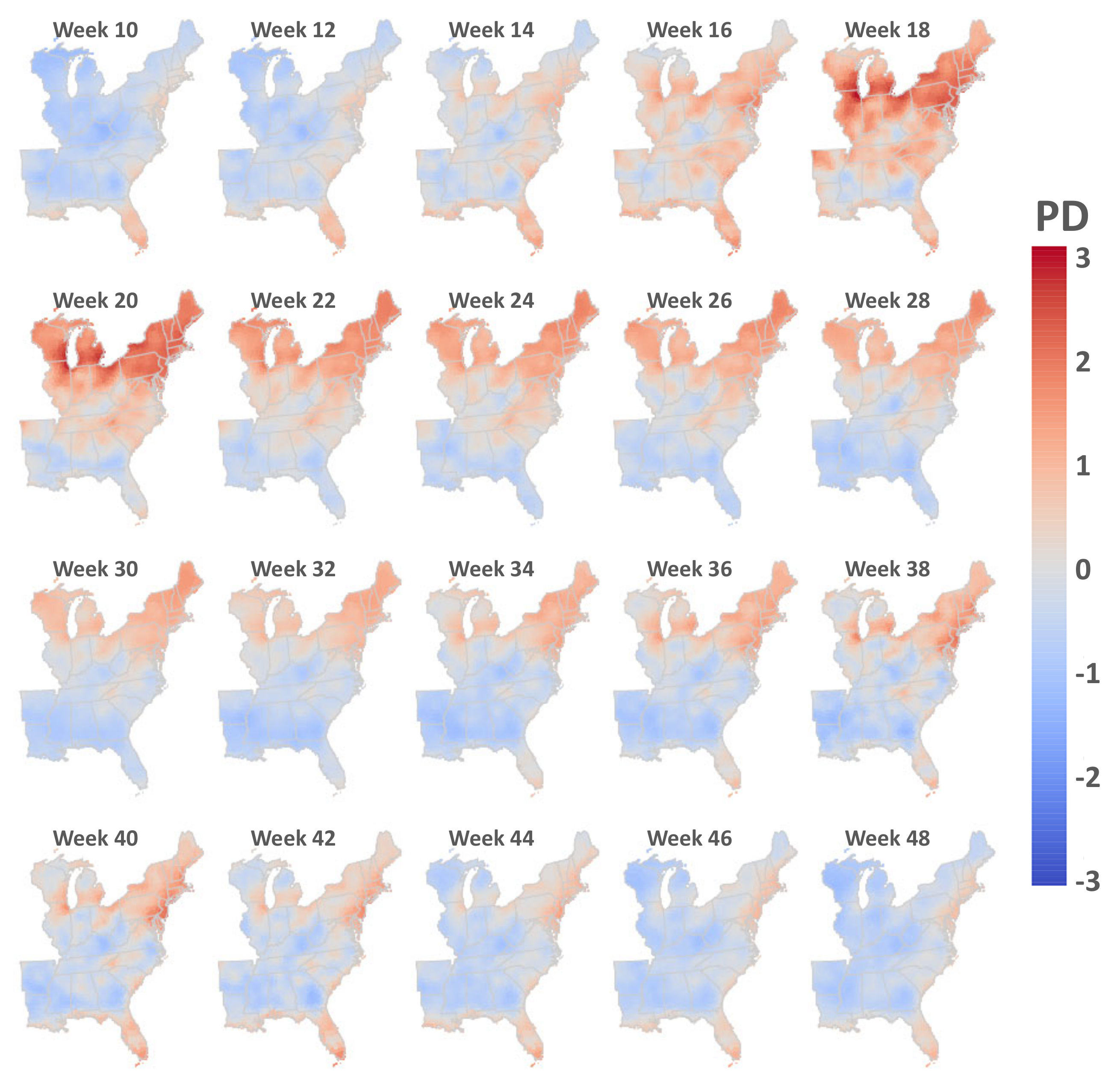
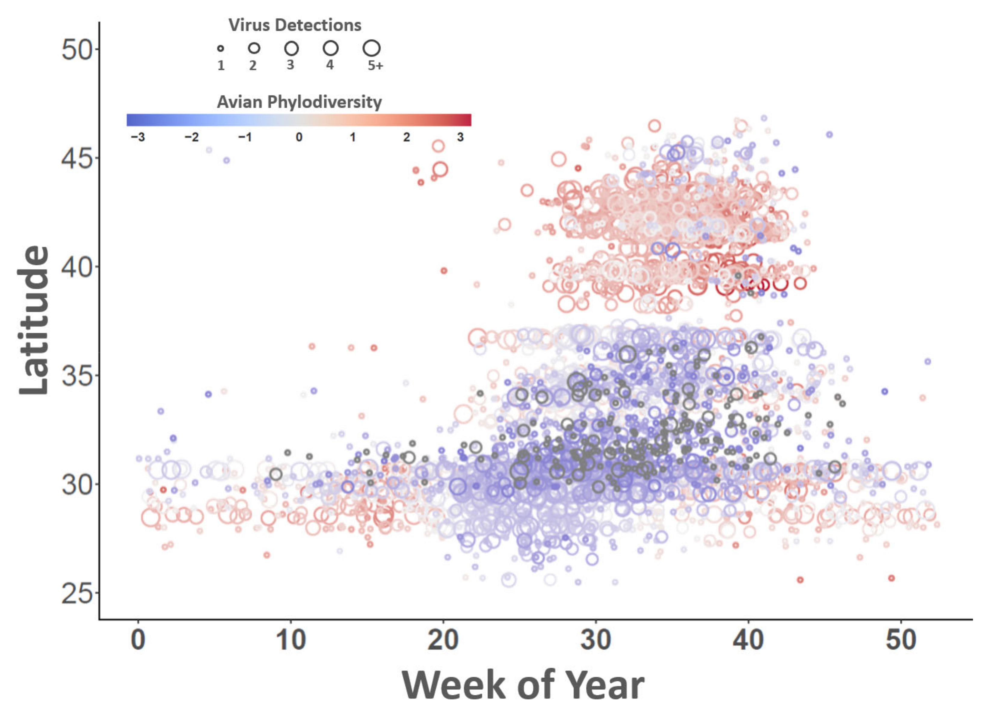
Avian-community phylogenetics, when combined with documented passerine-occurrence information, enabled avian-host phylodiversity (PD) to be dynamically mapped for the entire study area in weekly time steps (Figure 3). As shown in Figure 3, the average relatedness among avian-host communities was found to vary across the study area and through time, as species composition changed throughout the year. When matched to times and locations with confirmed EEEv detections, the overall distribution shown by the graphed detections encapsulate the EEE outbreak season (Figure 4). Figure 4 also highlights that a latitudinal break in EEEv–PD relationships exists at approximately 37.5 N latitude (the state of Virginia). The latitudinal break in EEEv–PD correspondence suggests that late-season EEEv detections northward of the break were associated with relatively high PD, whereas points below the break were mostly associated with lower PD.
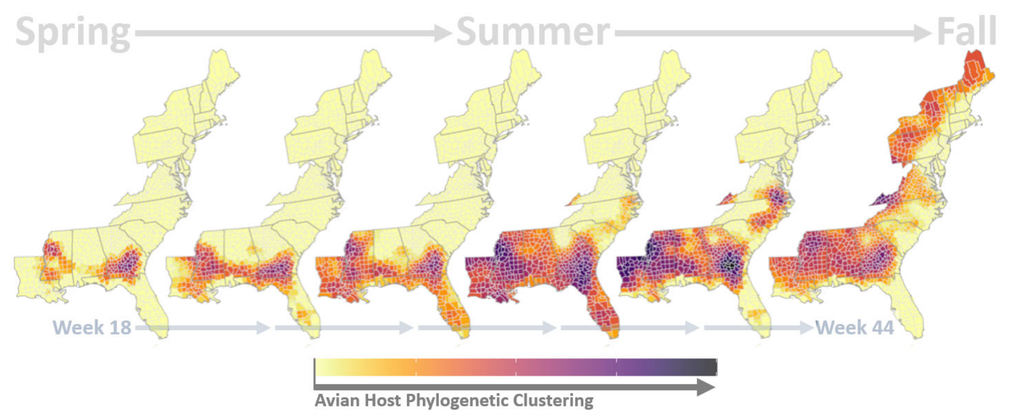
Remapping phylogenetically clustered areas (negative values from Figure 3) along coastal portions of the study area aided in visualizing how possible dilution effects may drive EEEv distributions during the primary EEE season (Figure 5). Figure 5 illustrates that southern Georgia, the Florida Panhandle (the western-most portion of state), and other locations along the Gulf of Mexico exhibit strong avian-host phylogenetic clustering at the beginning of the EEE outbreak season (locations shown with dark tones in Week 18 panel, early May) and that these clustered areas expand laterally and northward as the EEE season progresses through late summer and fall (Week 44, late October). The overall spatiotemporal trend suggested by host phylogenetic clustering is one of movement and diffusion from southern locations to northern locations, such that New England avian communities become more genetically similar at the end of summer and early fall. To better illustrate the information in Figure 5, larger weekly maps and video animations are provided with other supporting information at this article’s data repository site (Video 2, https://osf.io/tw2e9/, accessed on 7 July 2022).
Model comparison revealed that Model 15, which included all spatiotemporal effects (Equation (4)) and a Type-IV space–time interaction, exhibited the best overall parsimony, as judged by the DIC, WAIC, and lCPO (Table 2). A Type-IV interaction was also identified as outperforming other interaction types among those models with structured spatial effects not indexed by time (Models 8–11). Despite the additional model complexity created by adding spatiotemporal effects, model comparison also demonstrated that models with spatiotemporal effects exhibited greater parsimony than the fixed-effects-only model (Model 1). The DIC, WAIC, and lCPO for all models are detailed in Table 2.
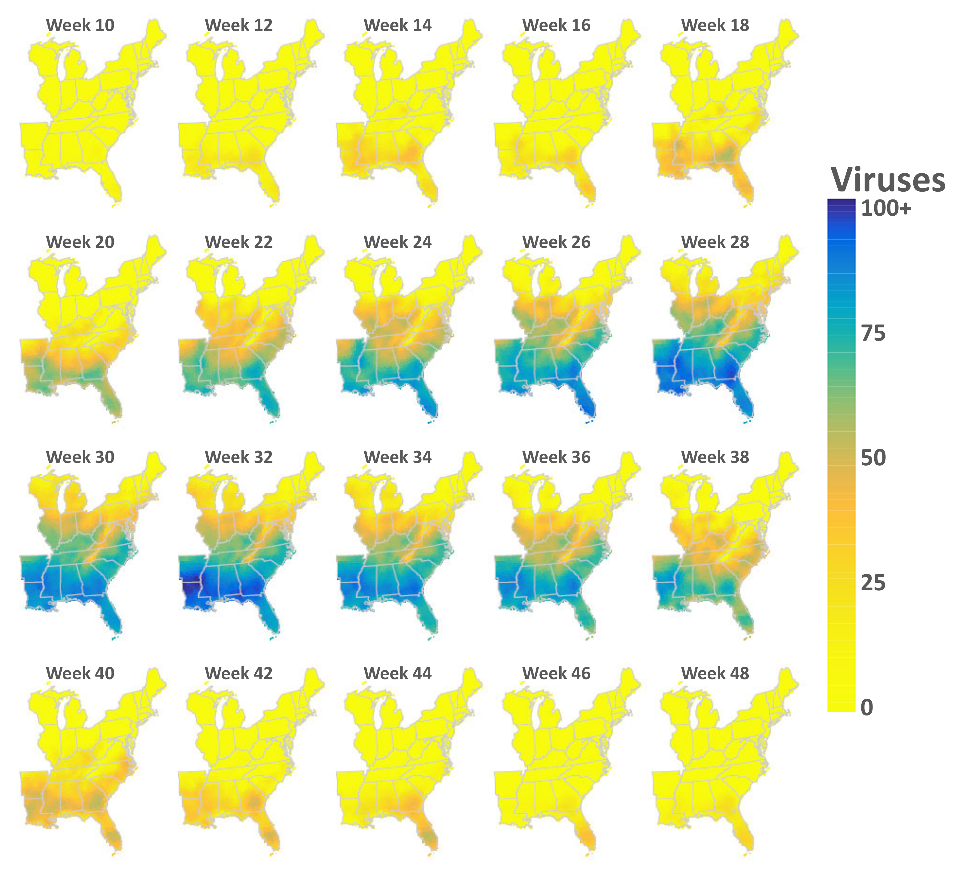
EEEv counts, as predicted by the best performing model (Model 15), are shown for select weeks of the year in Figure 6. The overall pattern of predicted EEEv counts suggested a trend in which viruses were restricted to southern latitudes and coastal regions prior to Week 10 (early March), moved northward through Week 36 (early September), and then receded southward and towards coasts by Week 44 (early November). Counties in Peninsular Florida were predicted to have viruses throughout the majority of the year; however, the number of viruses increased sharply from Week 18 through Week 40. Individual maps for each week of the year and video animations depicting data shown in Figure 6 are provided with other supporting information at this article’s data repository site (Video 3, https://osf.io/tw2e9/, accessed on 7 July 2022).
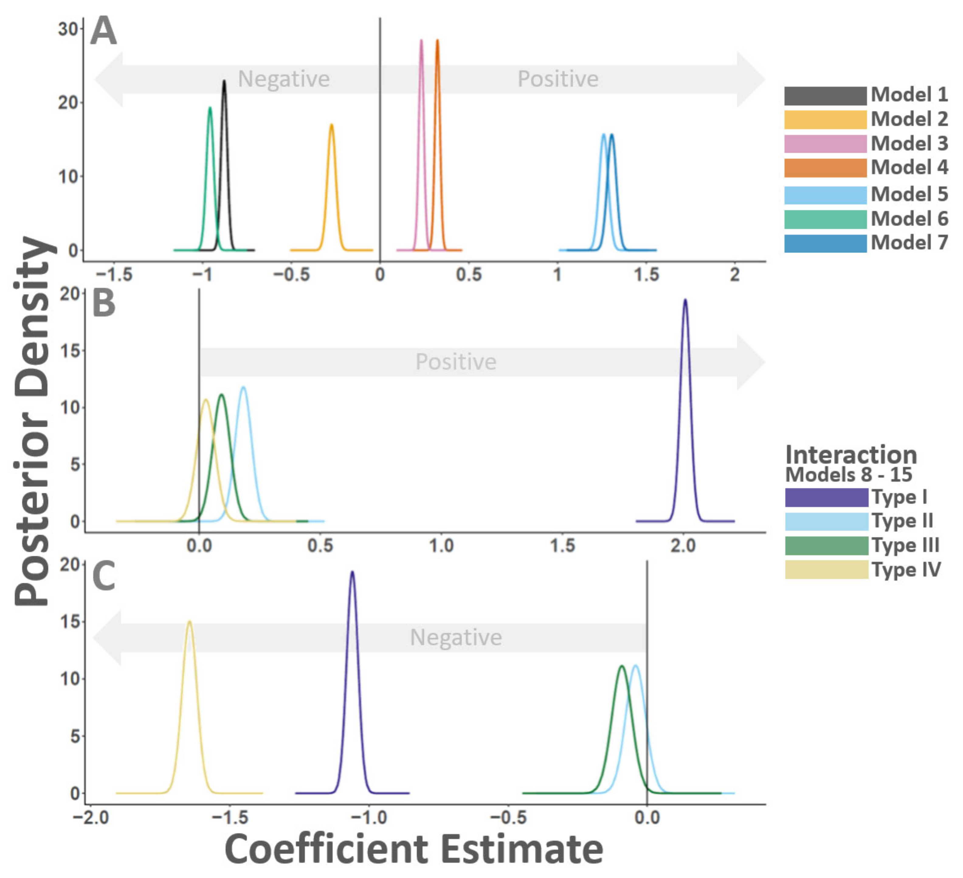
All models estimated temperature and precipitation to have a positive effect on EEEv occurrence. The average coefficient for temperature was 4.07 (0.03 sd, (3.89, 4.35) 95% CI) and the average coefficient for precipitation was 0.05 (0.01 sd, (0.04, 0.06) 95% CI). Although models uniformly indicated a positive relationship for climate effects, coefficient magnitudes and polarity (positive or negative sign) estimated for PD varied by model and the specific implementation of spatiotemporal effects. Figure 7 plots the posterior densities for PD as estimated by all models. PD effects from all models were judged to be statistically important based on 95% credible intervals excluding zero; however, Models 3–5, Model 7, and Models 8–11 suggested a positive relationship between PD and EEEv (i.e., an amplification effect), whereas Models 1–2, Model 6, and Models 12–15 suggested a negative EEEv–PD correspondence consistent with a dilution effect.
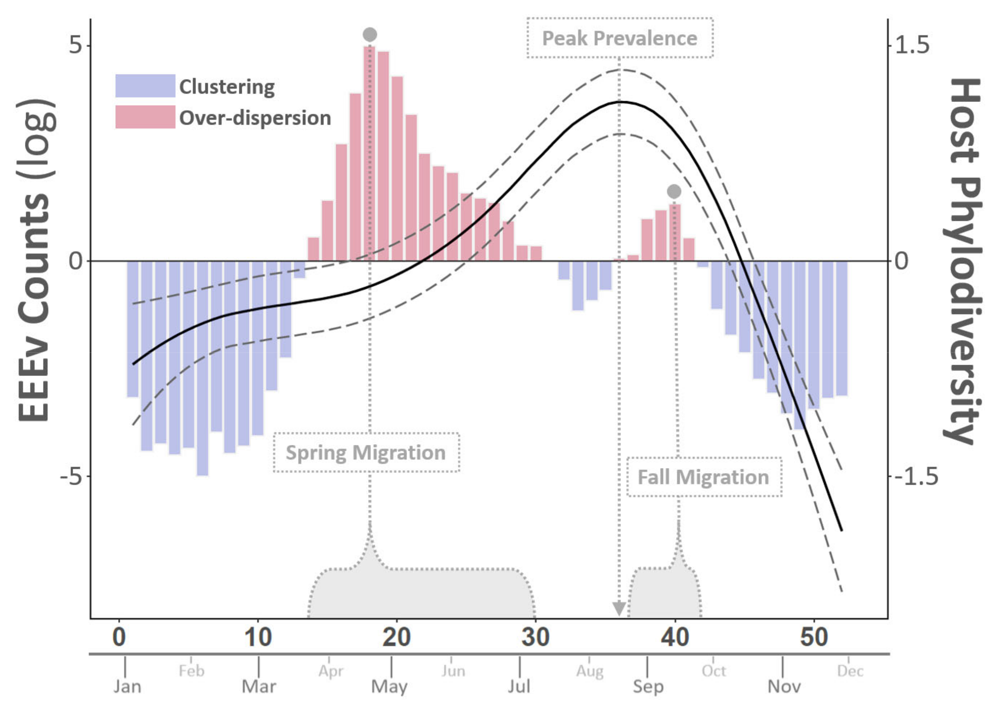
Comparison of EEEv counts and PD through time indicated that EEEv rates appear to be positively correlated with changes in host phyodiversity between weeks 5–20 of the year, during which time both show increasing trends, as well as between weeks 40–52, when both show decreasing trends (Figure 8). Additionally, temporal PD trends were also suggestive of shifts in avian community composition associated with the spring and fall seasonal bird migrations. These findings are explored further in the discussion section.

4. Discussion

The principal conclusion drawn from the above analysis is that EEEv intra-annual variability shows a scale-dependent dilution effect such that virus prevalence is comparatively less at locations of elevated passerine phylodiversity (over-dispersion) than at places exhibiting phylogenetic clustering (decreased phylodiversity). Importantly, however, dilution effects observed in geographic space may be statistically masked by apparent amplification effects that transpire in the temporal dimension as increasing virus detections are made in concert with passerine-host movements and migrations. The general pattern suggested by these results is that, while the EEE outbreak season progresses from spring to summer, recently overwintered passerines move from thermally buffered coastal areas and southerly portions of the study domain to inland and more northern localities, effectively diffusing viruses and redistributing avian diversity from relatively concentrated winter habitats to more expansive foraging and breeding grounds throughout the eastern US (Figure 3 and Figure 8). In the US, passerines lacking cold-tolerance traits migrate to southern latitudes and coastal areas in winter to evade heavy snowfall and extreme low temperatures [60]. From the perspective of inland and northern locations, spring brings both migrant influx and elevated virus detection rates, giving the impression of an amplification effect; however, this amplification may only be apparent because, although virus detections increase moving into the height of the outbreak season, these detections largely consist of initial virus introductions rather than host amplification (replication). When the EEE outbreak season and eastern US are viewed as a whole, EEEv peak prevalence is actually observed 15–20 weeks following the height of the spring migration, prior to the fall migration, and during a period associated with the passerine breeding season and community phylogenetic clustering (Figure 5 and Figure 8). Assuming passerine physiologic traits, behaviors, and niches at least partially mediate transmission processes and are correlated with interspecies relatedness (i.e., phylogenetic conservatism sensu Wiens and Graham [61]), phylogenetically clustered communities afford greater opportunity for virus sharing, host switching, and spillover than do over-dispersed communities.
Several crucial caveats must be made regarding the interpretation of the modeling results. The finding of an EEEv dilution effect was based on the domain-wide, average influence of passerine phylodiversity as estimated for the period 2002–2019. EEEv–PD correspondence assessed over different geographic extents or using other time windows may reach a different conclusion, irrespective of the specific statistical implementation adopted for analysis. As a case in point, large portions of New England showed high EEEv abundances in late summer (after Week 35, Figure 6), a time period actively trending towards decreased passerine PD (Figure 3) but still exhibiting above average levels of phylogenetic over-dispersion (Figure 4). Had these New England regions been modeled independently of the reminder of the EEEv range, model results would have indicated an amplification effect and drawn the opposite conclusion than that presented here for the Eastern US in its entirety.
Regarding New England specifically, other studies have reported a similar late-season dynamic in response to increased EEEv detections in migratory passerines [7], elevated EEEv seroprevalance among late-summer passerine hatchlings [62], large mosquito broods at the end of summer [63], and other late-season passerine-mosquito interactions [64,65]. Although the scope of the current study is insufficient to confirm any of these mechanisms precisely, it does corroborate the existence of a late-season New England dynamic partly out of sync with EEEv in the eastern US as a whole. For example, the proportion of New-England counties experiencing host-phylogenetic clustering was found to sharply increase at the end of summer, suggesting a rapid upswing in bird movement northward from central Atlantic states and locations further south (Figure 5, last two panels at right). In addition to the possible increased proliferation of the virus among less phylogenetically distant species, late-season migrant influx may also introduce new viruses. Consistent with several genetic studies [66,67,68], this analysis lends macroecological support to the notion of passerine communities moving the virus from source locations in southern Georgia, Mississippi, and the Florida Panhandle to virus sinks in New England.
Finally, models based on stationary spatial patterns (Models 8–11, Figure 7), incorporating smooth temporal trends in the absence of spatial effects (Models 3–4, Figure 7), or implementing time as a simple factor variable (Model 5, Figure 7) would have drawn different conclusions than made here for EEEv–PD relationships. In fact, models constructed under these assumptions produced the opposite results, indicating an amplification effect rather than a dilution effect. This finding highlights that spatiotemporal analysis of complex ecological data can be prone to misinterpretation and that decisions researchers make when implementing spatial and temporal covariates have major implications for results and how those results are interpreted. Although the current study emphasized the need to exercise caution in choosing model inputs and interpreting outputs, it was limited by incomplete and uneven virus observation data and would have benefited from the inclusion of additional facets of the EEEv system, particularly, vector mosquito-occurrence data.

5. Conclusions

This study applied seventeen years of non-human EEEv detections to quantify dilution and amplification effects in response to passerine-host phylodiversity. Results indicated that increased avian phylodiversity promotes EEEv dilution across geographic space, but observed virus-dilution effects are scale-dependent and may be concealed by concurrent amplification effects that occur through the height of the summer outbreak season. Findings further demonstrated that statistical modeling decisions related to how spatial, temporal, and space–time interaction effects are included in analysis have major impacts on model outcomes and can lead to results misinterpretation even when arithmetic and mathematics are technically correct. Recent evidence suggests that the geographic range of EEEv may be expanding and contributing to increased virus infection rates in humans, livestock, and wildlife; therefore, it is imperative that the interconnections between people, animals, and the shared environment be recognized to improve EEEv surveillance and better anticipate future EEE disease outbreaks from a One Health perspective.

Funding

This work was supported by the USDA ARS Northern Plains Agricultural Research Laboratory, Pest Management Research Unit and CRIS Project 3032-22000-019-000-D.

Data Availability Statement

Weekly estimates for passerine phyodiversity and virus prevalence produced by this study are freely available for download as GeoTIFF files from the Open Science Framework (OSF) data repository (https://osf.io/tw2e9/, accessed on 7 July 2022). Animated videos and additional map figures depicting results are also available at the OSF website. Original virus detection data can be obtained from the Centers for Disease Control and Prevention (CDC) [35].

Acknowledgments

This research used resources provided by the SCINet project of the USDA Agricultural Research Service, ARS project number 0500-00093-001-00-D. Mention of trade names or commercial products in this publication is solely for the purpose of providing specific information and does not imply recommendation or endorsement by the US Department of Agriculture. The conclusions of this report are those of the authors and do not necessarily represent the views of the USDA. USDA is an equal opportunity provider and employer.

Conflicts of Interest

The author declares no conflict of interest.

References

  1. Armstrong, P.M.; Andreadis, T.G. Eastern equine encephalitis virus—Old enemy, new threat. N. Engl. J. Med. 2013, 368, 1670–1673. [Google Scholar] [CrossRef] [PubMed] [Green Version]
  2. Burkett-Cadena, N.D.; Day, J.F.; Unnasch, T.R. Ecology of Eastern Equine Encephalitis Virus in the Southeastern United States: Incriminating Vector and Host Species Responsible for Virus Amplification, Persistence, and Dispersal. J. Med. Entomol. 2021, 59, 41–48. [Google Scholar] [CrossRef] [PubMed]
  3. Tang, X.; Sedda, L.; Brown, H.E. Predicting eastern equine encephalitis spread in North America: An ecological study. Curr. Res. Parasitol.-Vector-Borne Dis. 2021, 1, 100064. [Google Scholar] [CrossRef] [PubMed]
  4. Animal and Plant Health Inspection Service (APHIS). Equine Encephalitis. 2021. Available online: https://www.aphis.usda.gov/aphis/ourfocus/animalhealth/animal-disease-information/equine/eee-wee-vee (accessed on 14 December 2021).
  5. Villari, P.; Spielman, A.; Komar, N.; McDowell, M.; Timperi, R.J. The Economic Burden Imposed by a Residual Case of Eastern Encephalitis. Am. J. Trop. Med. Hyg. 1995, 52, 8–13. [Google Scholar] [CrossRef] [PubMed]
  6. Armstrong, P.M.; Andreadis, T.G. Ecology and Epidemiology of Eastern Equine Encephalitis Virus in the Northeastern United States: An Historical Perspective. J. Med. Entomol. 2021, 59, 1–13. [Google Scholar] [CrossRef]
  7. Davis, W.A. A study of birds and mosquitoes as hosts for the virus of eastern equine encephalomyelitis. Am. J. Hyg. 1940, 32, 45–59. [Google Scholar]
  8. Scott, T.W.; Weaver, S.C. Eastern equine encephalomyelitis virus: Epidemiology and evolution of mosquito transmission. Adv. Virus Res. 1989, 37, 277–328. [Google Scholar]
  9. Komar, N.; Dohm, D.J.; Turell, M.J.; Spielman, A. Eastern equine encephalitis virus in birds: Relative competence of European starlings (Sturnus vulgaris). Am. J. Trop. Med. Hyg. 1999, 60, 387–391. [Google Scholar] [CrossRef]
  10. Weaver, S.C.; Barrett, A.D.T. Transmission cycles, host range, evolution and emergence of arboviral disease. Nat. Rev. Microbiol. 2004, 2, 789–801. [Google Scholar] [CrossRef]
  11. Alatoom, A.; Payne, D. An Overview of Arboviruses and Bunyaviruses. Lab. Med. 2009, 40, 237–240. [Google Scholar] [CrossRef] [Green Version]
  12. Go, Y.Y.; Balasuriya, U.B.R.; Lee, C.-k. Zoonotic encephalitides caused by arboviruses: Transmission and epidemiology of alphaviruses and flaviviruses. Clin. Exp. Vaccine Res. 2014, 3, 58–77. [Google Scholar] [CrossRef] [Green Version]
  13. Wong, K.T. Alphaviral Equine Encephalomyelitis (Eastern, Western, and Venezuelan). In Infections of the Central Nervous System; John Wiley & Sons, Ltd.: Hoboken, NJ, USA, 2020. [Google Scholar] [CrossRef]
  14. Stenkamp-Strahm, C.; Patyk, K.; McCool-Eye, M.J.; Fox, A.; Humphreys, J.; James, A.; South, D.; Magzamen, S. Using geospatial methods to measure the risk of environmental persistence of avian influenza virus in South Carolina. Spat. Spatio Temporal Epidemiol. 2020, 34, 100342. [Google Scholar] [CrossRef]
  15. Humphreys, J.M.; Ramey, A.M.; Douglas, D.C.; Mullinax, J.M.; Soos, C.; Link, P.; Walther, P.; Prosser, D.J. Waterfowl occurrence and residence time as indicators of H5 and H7 avian influenza in North American Poultry. Sci. Rep. 2020, 10, 1–16. [Google Scholar] [CrossRef]
  16. Ramey, A.M.; Reeves, A.B.; Drexler, J.Z.; Ackerman, J.T.; De La Cruz, S.; Lang, A.S.; Leyson, C.; Link, P.; Prosser, D.J.; Robertson, G.J.; et al. Influenza A viruses remain infectious for more than seven months in northern wetlands of North America. Proc. R. Soc. Biol. Sci. 2020, 287, 20201680. [Google Scholar] [CrossRef]
  17. Tolsá, M.J.; García-Peña, G.E.; Rico-Chávez, O.; Roche, B.; Suzán, G. Macroecology of birds potentially susceptible to West Nile virus. Proc. R. Soc. Biol. Sci. 2018, 285. [Google Scholar] [CrossRef] [Green Version]
  18. Humphreys, J.M.; Pelzel-McCluskey, A.M.; Cohnstaedt, L.W.; McGregor, B.L.; Hanley, K.A.; Hudson, A.R.; Young, K.I.; Peck, D.; Rodriguez, L.L.; Peters, D.P.C. Integrating Spatiotemporal Epidemiology, Eco-Phylogenetics, and Distributional Ecology to Assess West Nile Disease Risk in Horses. Viruses 2021, 13, 1811. [Google Scholar] [CrossRef]
  19. Suzán, G.; García-Peña, G.E.; Castro-Arellano, I.; Rico, O.; Rubio, A.V.; Tolsá, M.J.; Roche, B.; Hosseini, P.R.; Rizzoli, A.; Murray, K.A.; et al. Metacommunity and phylogenetic structure determine wildlife and zoonotic infectious disease patterns in time and space. Ecol. Evol. 2015, 5, 865–873. [Google Scholar] [CrossRef]
  20. Huang, Z.Y.X.; de Boer, W.F.; van Langevelde, F.; Olson, V.; Blackburn, T.M.; Prins, H.H.T. Species’ Life-History Traits Explain Interspecific Variation in Reservoir Competence: A Possible Mechanism Underlying the Dilution Effect. PLoS ONE 2013, 8, e54341. [Google Scholar] [CrossRef] [Green Version]
  21. Keesing, F.; Holt, R.D.; Ostfeld, R.S. Effects of species diversity on disease risk. Ecol. Lett. 2006, 9, 485–498. [Google Scholar] [CrossRef]
  22. Kramer, L.D.; Ciota, A.T.; Marm Kilpatrick, A. Introduction, Spread, and Establishment of West Nile Virus in the Americas. J. Med. Entomol. 2019, 56, 1448–1455. [Google Scholar] [CrossRef]
  23. Ogden, N.; Tsao, J. Biodiversity and Lyme disease: Dilution or amplification? Epidemics 2009, 1, 196–206. [Google Scholar] [CrossRef] [PubMed]
  24. Randolph, S.E.; Dobson, A.D. Pangloss revisited: A critique of the dilution effect and the biodiversity-buffers-disease paradigm. Parasitology 2012, 139, 847–863. [Google Scholar] [CrossRef] [PubMed]
  25. Mihaljevic, J.R.; Joseph, M.B.; Orlofske, S.A.; Paull, S.H. The Scaling of Host Density with Richness Affects the Direction, Shape, and Detectability of Diversity-Disease Relationships. PLoS ONE 2014, 9, e97812. [Google Scholar] [CrossRef] [PubMed] [Green Version]
  26. Huang, Z.; Van Langevelde, F.; Estrada-Peña, A.; Suzán, G.; De Boer, W. The diversity–disease relationship: Evidence for and criticisms of the dilution effect. Parasitology 2016, 143, 1075–1086. [Google Scholar] [CrossRef]
  27. Norman, R.; Bowers, R.; Begon, M.; Hudson, P.J. Persistence of tick-borne virus in the presence of multiple host species: Tick reservoirs and parasite mediated competition. J. Theor. Biol. 1999, 200, 111–118. [Google Scholar] [CrossRef] [Green Version]
  28. Ostfeld, R.S.; Keesing, F. Biodiversity and Disease Risk: The Case of Lyme Disease. Conservation Biology 2000, 14, 722–728. [Google Scholar] [CrossRef]
  29. Estrada-Peña, A. The relationships between habitat topology, critical scales of connectivity and tick abundance Ixodes ricinus in a heterogeneous landscape in northern Spain. Ecography 2003, 26, 661–671. [Google Scholar] [CrossRef]
  30. Humphreys, J.M.; Young, K.I.; Cohnstaedt, L.W.; Hanley, K.A.; Peters, D.P.C. Vector Surveillance, Host Species Richness, and Demographic Factors as West Nile Disease Risk Indicators. Viruses 2021, 13, 934. [Google Scholar] [CrossRef]
  31. Abellan, J.J.; Richardson, S.; Best, N. Use of Space & Time Models to Investigate the Stability of Patterns of Disease. Environ. Health Perspect. 2008, 116, 1111–1119. [Google Scholar] [CrossRef] [Green Version]
  32. Knorr-Held, L. Bayesian modelling of inseparable space-time variation in disease risk. Stat. Med. 2000, 19, 2555–2567. [Google Scholar] [CrossRef] [Green Version]
  33. Humphreys, J.M.; Mahjoor, A.; Reiss, K.C.; Uribe, A.A.; Brown, M.T. A geostatistical model for estimating edge effects and cumulative human disturbance in wetlands and coastal waters. Int. J. Geogr. Inf. Sci. 2020, 34, 1508–1529. [Google Scholar] [CrossRef]
  34. Briz-Redón, Á. The impact of modelling choices on modelling outcomes: A spatio-temporal study of the association between COVID-19 spread and environmental conditions in Catalonia (Spain). Stoch. Environ. Res. Risk Assess. 2021, 35, 1701–1713. [Google Scholar] [CrossRef]
  35. Centers for Disease Control and Prevention (CDC). ArboNET. 2021. Available online: https://wwwn.cdc.gov/arbonet (accessed on 14 December 2021).
  36. PRISM. Total Annual Precipitation and Mean Maximum Temperature Climate Data. 2020. Available online: http://prism.oregonstate.edu (accessed on 12 June 2020).
  37. Sullivan, B.L.; Aycrigg, J.L.; Barry, J.H.; Bonney, R.E.; Bruns, N.; Cooper, C.B.; Damoulas, T.; Dhondt, A.A.; Dietterich, T.; Farnsworth, A.; et al. The eBird enterprise: An integrated approach to development and application of citizen science. Biol. Conserv. 2014, 169, 31–40. [Google Scholar] [CrossRef]
  38. Jetz, W.; Thomas, G.H.; Joy, J.B.; Hartmann, K.; Mooers, A.O. The global diversity of birds in space and time. Nature 2012, 491, 444–448. [Google Scholar] [CrossRef]
  39. Bouckaert, R.; Heled, J.; Kühnert, D.; Vaughan, T.; Wu, C.H.; Xie, D.; Suchard, M.A.; Rambaut, A.; Drummond, A.J. BEAST 2: A Software Platform for Bayesian Evolutionary Analysis. PLoS Comput. Biol. 2014, 10, e1003537. [Google Scholar] [CrossRef] [Green Version]
  40. Kembel, S.; Cowan, P.; Helmus, M.; Cornwell, W.; Morlon, H.; Ackerly, D.; Blomberg, S.; Webb, C. Picante: R tools for integrating phylogenies and ecology. Bioinformatics 2010, 26, 1463–1464. [Google Scholar] [CrossRef] [Green Version]
  41. Larsen, A.E.; Meng, K.; Kendall, B.E. Causal analysis in control–impact ecological studies with observational data. Methods Ecol. Evol. 2019, 10, 924–934. [Google Scholar] [CrossRef]
  42. Laubach, Z.M.; Murray, E.J.; Hoke, K.L.; Safran, R.J.; Perng, W. A biologist’s guide to model selection and causal inference. Proc. R. Soc. Biol. Sci. 2021, 288, 20202815. [Google Scholar] [CrossRef]
  43. Meisner, J.; Kato, A.; Lemerani, M.; Miaka, E.M.; Taban, A.I.; Wakefield, J.; Rowhani-Rahbar, A.; Pigott, D.; Mayer, J.; Rabinowitz, P. Livestock, pathogens, vectors, and their environment: A causal inference-based approach to estimating the pathway-specific effect of livestock on human African trypanosomiasis risk. medRxiv 2022, 1, 1–17. [Google Scholar] [CrossRef]
  44. Humphreys, J.M.; Srygley, R.B.; Lawton, D.; Hudson, A.R.; Branson, D.H. Grasshoppers exhibit asynchrony and spatial non-stationarity in response to the El Niño/Southern and Pacific Decadal Oscillations. Ecol. Model. 2022, 471, 110043. [Google Scholar] [CrossRef]
  45. Bivand, R.; Piras, G. Comparing Implementations of Estimation Methods for Spatial Econometrics. J. Stat. Softw. 2015, 63, 1–36. [Google Scholar] [CrossRef] [Green Version]
  46. Simpson, D.; Rue, H.; Riebler, A.; Martins, T.G.; Sørbye, S.H. Penalising Model Component Complexity: A Principled, Practical Approach to Constructing Priors. Stat. Sci. 2017, 32, 1–28. [Google Scholar] [CrossRef]
  47. Riebler, A.; Sørbye, S.H.; Simpson, D.; Rue, H.; Lawson, A.B.; Lee, D.; MacNab, Y. An intuitive Bayesian spatial model for disease mapping that accounts for scaling. Stat. Methods Med. Res. 2016, 25, 1145–1165. [Google Scholar] [CrossRef] [Green Version]
  48. Humphreys, J.M.; Douglas, D.C.; Ramey, A.M.; Mullinax, J.M.; Soos, C.; Link, P.; Walther, P.; Prosser, D.J. The spatial-temporal relationship of blue-winged teal to domestic poultry: Movement state modeling of a highly mobile avian influenza host. J. Appl. Ecol. 2021, 58, 2040–2052. [Google Scholar] [CrossRef]
  49. Blangiardo, M.; Cameletti, M. Spatial and Spatio-Temporal Bayesian Models with R-INLA; John Wiley & Sons, Inc.: Chichester, UK, 2015. [Google Scholar]
  50. Rue, H.; Martino, S.; Chopin, N. Approximate Bayesian inference for latent Gaussian models by using integrated nested Laplace approximations. J. R. Stat. Soc. Ser. Stat. Methodol. 2009, 71, 319–392. [Google Scholar] [CrossRef]
  51. Martins, T.G.; Simpson, D.; Lindgren, F.; Rue, H. Bayesian computing with INLA: New features. Comput. Stat. Data Anal. 2013, 67, 68–83. [Google Scholar] [CrossRef] [Green Version]
  52. Lindgren, F.; Rue, H. Bayesian Spatial Modelling with R-INLA. J. Stat. Softw. 2015, 63, 1–25. [Google Scholar] [CrossRef] [Green Version]
  53. Verbosio, F.; De Coninck, A.; Kourounis, D.; Schenk, O. Enhancing the scalability of selected inversion factorization algorithms in genomic prediction. J. Comput. Sci. 2017, 22, 99–108. [Google Scholar] [CrossRef]
  54. Kourounis, D.; Fuchs, A.; Schenk, O. Towards the Next Generation of Multiperiod Optimal Power Flow Solvers. IEEE Trans. Power Syst. 2018, 33, 4005–4014. [Google Scholar] [CrossRef]
  55. Van Niekerk, J.; Bakka, H.; Rue, H.; Schenk, O. New frontiers in Bayesian modeling using the INLA package in R. arXiv 2019, arXiv:1907.10426. [Google Scholar] [CrossRef]
  56. Gelman, A.; Hwang, J.; Vehtari, A. Understanding predictive information criteria for Bayesian models. Stat. Comput. 2014, 24, 997–1016. [Google Scholar] [CrossRef]
  57. Gneiting, T.; Raftery, A.E. Strictly Proper Scoring Rules, Prediction, and Estimation. J. Am. Stat. Assoc. 2007, 102, 359–378. [Google Scholar] [CrossRef]
  58. Spiegelhalter, D.J.; Best, N.G.; Carlin, B.P.; Van Der Linde, A. Bayesian measures of model complexity and fit. J. R. Stat. Soc. Ser. Stat. Methodol. 2002, 64, 583–639. [Google Scholar] [CrossRef] [Green Version]
  59. Hooten, M.B.; Hobbs, N.T. A guide to Bayesian model selection for ecologists. Ecol. Monogr. 2015, 85, 3–28. [Google Scholar] [CrossRef]
  60. Dawson, W.R.; Marsh, R.L.; Yacoe, M.E. Metabolic adjustments of small passerine birds for migration and cold. Am. J. Physiol. Regul. Integr. Comp. Physiol. 1983, 245, R755–R767. [Google Scholar] [CrossRef]
  61. Wiens, J.J.; Graham, C.H. Niche Conservatism: Integrating Evolution, Ecology, and Conservation Biology. Annu. Rev. Ecol. Evol. Syst. 2005, 36, 519–539. [Google Scholar] [CrossRef] [Green Version]
  62. Elias, S.P.; Keenan, P.; Kenney, J.L.; Morris, S.R.; Covino, K.M.; Robinson, S.; Foss, K.A.; Rand, P.W.; Lubelczyk, C.; Lacombe, E.H.; et al. Seasonal patterns in eastern equine encephalitis virus antibody in songbirds in southern Maine. Vector-Borne Zoonotic Dis. 2017, 17, 325–330. [Google Scholar] [CrossRef]
  63. Edman, J.; Timperi, R.; Werner, B. Epidemiology of eastern equine encephalitis in Massachusetts. J. Fla. Mosq. Control. Assoc. 1993, 64, 84–96. [Google Scholar]
  64. Morris, C.D.; Zimmerman, R.H.; Edman, J.D. Epizootiology of Eastern Equine Encephalomyelitis Virus in Upstate New York, USA: II. Population dynamics and vector potential of adult Culiseta melanura (Diptera: Culicidae) in relation to distance from breeding site. J. Med. Entomol. 1980, 17, 453–465. [Google Scholar] [CrossRef]
  65. Morris, C.D.; Zimmerman, R.H. Epizootiology of Eastern Equine Encephalomyelitis Virus in Upstate New York, USA: III. Population dynamics and vector potential of adult Culiseta morsitans (Diptera: Culicidae). J. Med. Entomol. 1981, 18, 313–316. [Google Scholar] [CrossRef] [Green Version]
  66. Armstrong, P.M.; Andreadis, T.G.; Anderson, J.F.; Stull, J.W.; Mores, C.N. Tracking eastern equine encephalitis virus perpetuation in the northeastern United States by phylogenetic analysis. Am. J. Trop. Med. Hyg. 2008, 79, 291–296. [Google Scholar] [CrossRef] [Green Version]
  67. Young, D.S.; Kramer, L.D.; Maffei, J.G.; Dusek, R.J.; Backenson, P.B.; Mores, C.N.; Bernard, K.A.; Ebel, G.D. Molecular epidemiology of eastern equine encephalitis virus, New York. Emerg. Infect. Dis. 2008, 14, 454. [Google Scholar] [CrossRef]
  68. Tan, Y.; Lam, T.T.Y.; Heberlein-Larson, L.A.; Smole, S.C.; Auguste, A.J.; Hennigan, S.; Halpin, R.A.; Fedorova, N.; Puri, V.; Stockwell, T.B.; et al. Large-Scale Complete-Genome Sequencing and Phylodynamic Analysis of Eastern Equine Encephalitis Virus Reveals Source-Sink Transmission Dynamics in the United States. J. Virol. 2018, 92, e00074-18. [Google Scholar] [CrossRef] [Green Version]
Figure 1. EEEv detections in non-human hosts. Bar graph depicts the annual number of EEEv detections for the seventeen-year period of record (2003–2019). Horizontal axis lists detection year and vertical axis gives count of total EEEv detections. Vertical bars are color-coded to indicate EEEv detections made from mosquito, mammal, sentinel chicken, and wild-bird hosts.
Geographies 02 00026 g001
Figure 2. Graphical model of avian-host diversity relationships to EEEv. Directed acyclic graph (DAG) nodes symbolize observed and unobserved aspects of the diversity-EEEv system with arrows indicating hypothesized causal relationships. Nodes represent host diversity (HD), true EEEv prevalence (V) in the environment, and human documented EEEv detections (D). Also included in the heuristic are spatial (S), temporal (T), and space–time interaction (I) processes, as well as, temperature (TMP), precipitation (PPT), and exposure (E) effects. Nodes shown with dashed borders (gray shading) signify unobserved variables that must be estimated through statistical modeling, whereas nodes with solid borders indicate variables with available data proxies.
Geographies 02 00026 g002
Figure 3. Estimated avian-host phylodiversity. Maps depict the study domain for select weeks of the year and are color-coded according to legend at right to indicate relative phylodiversity (PD) by county and week. PD values have been scaled and centered to show relative phylogenetic clustering with blue colors (higher than expected relatedness, lower mean genetic distances) and phylogenetic over-dispersion with red colors (lower than expected relatedness, higher mean genetic distances). Note that PD varies across geographic space and through time, as avian community composition varies throughout the year. Maps for each week of the year and video animations depicting PD changes through time can be viewed with other supporting information at this article’s data repository site (Video 1, https://osf.io/tw2e9/, accessed on 7 July 2022).
Geographies 02 00026 g003
Figure 4. Comparison of reported EEEv detections to avian-host phylodiversity. Figure graphs reported EEEv detections by geographic latitude (vertical axis) and week of year (horizontal axis) with coincident avian-host phylodiversity (PD). Each graph point represents an individual county and is color-coded according to inset legend (top left) to show the PD estimated for the county and week of virus detection. Points are sized to illustrate the approximate number of virus detections for that county and week. Latitudes were calculated from county geographic centers and all points were subject to 5% jittering to reduce overlap. Data cover the period 2003–2019; therefore, counties may be represented multiple times (i.e., the same county but in different years).
Geographies 02 00026 g004
Figure 5. Avian-host phylogenetic clustering. Maps depict coastal portions of the study domain during the primary EEE outbreak season. Counties are color-coded according to legend at bottom to indicate the relative intensity of avian-host phylogenetic clustering, with darker tones signifying that host communities are more genetically similar than expected by chance. Note strong phylogenetic clustering along the Gulf of Mexico near the beginning of the EEE outbreak season (Week 18, early May) with lateral and northward diffusion through late summer and fall (Week 44, late October). Maps for each week of the year and video animations depicting phylogenetic clustering changes through time can be viewed with other supporting information at this article’s data repository site (Video 2, https://osf.io/tw2e9/, accessed on 7 July 2022).
Geographies 02 00026 g005
Figure 6. Predicted EEEv counts. Maps depict the study domain for select weeks of the year and are color-coded according to legend at right to indicate the the number of EEEv predicted by county and week. Predictions were made using the best performing model (Model 15, Table 2). Maps for each week of the year and video animations depicting changes in virus prevalence through time can be viewed with other supporting information at this article’s data repository site (Video 3, https://osf.io/tw2e9/, accessed on 7 July 2022).
Geographies 02 00026 g006
Figure 7. Estimated avian-host phylodiversity effects. Figure illustrates the magnitude and polarity of avian-host-phylodiversity (PD) coefficients as estimated by all evaluated models. Horizontal axes list the estimated coefficient magnitude and the vertical line intersecting zero indicates polarity (positive or negative sign). Panel A shows PD estimates produced by Models 1–7, Panel B provides PD estimates given by Models 8–11, and Panel C shows PD estimates from Models 12–15. Posterior densities in Panel A are color-coded according to legend at immediate right; posterior densities in Panels B and C share the color scheme at bottom right, which corresponds to the spatiotemporal interaction type used in each model. Note that PD effects from all models were judged as statistically important based on 95% credible intervals excluding zero. Results from Models 3–5, 7, and 8–11 suggest a positive relationship between PD and EEEv (amplification effect), whereas Models 1–2, 6, and 12–15 suggest a negative EEEv–PD correspondence (dilution effect).
Geographies 02 00026 g007
Figure 8. EEEv and host-phylodiversity temporal comparison. Numbered values listed on horizontal axes give week of year and abbreviations approximate month. Solid curvilinear line corresponds to left vertical axis and depicts smoothed EEEv rate (counts, log scale) with parallel dashed lines signifying 95% credible interval for estimate. Vertical bars correspond to right vertical axis and show weekly average avian-host phylodiversity (one-dimensional version of estimates illustrated in Figure 3) with relative phylogenetic clustering (higher than expected relatedness, lower mean genetic distances) in blue and phylogenetic over-dispersion (lower than expected relatedness, higher mean genetic distances) in red. Figure is annotated to emphasize periods of over-dispersion associated with seasonal bird migrations and peak EEEv prevalence. EEEv rates are positively correlated to changes in phylodiversity between weeks 5–20 (both show increasing trends) and between weeks 40–52 (both show decreasing trends).
Geographies 02 00026 g008
Table 1. Space–time interaction type summary. First column labels the interaction type, second column lists spatial and temporal terms from Equation (4) relevant to the interaction type, third column notates the Kronecker product (⨂), and fourth column narratively describes spatial and temporal matrices. Unstructured spatial and temporal matrices are symbolized with the notation I (identity matrix) and structured matrices are shown as R.
InteractionParametersR δ Description
Type I υ s and ϕ t I υ I ϕ Unstructured space, unstructured time
Type II υ s and γ t I υ R γ Unstructured space, structured time
Type III u s and ϕ t R u I ϕ Structured space, unstructured time
Type IV u s and γ t R u R γ Structured space, structured time
Table 2. Model parsimony metrics. Deviance information criterion (DIC), Watanabe–Akaike information criterion (WAIC), and log-conditional predictive ordinate (lCPO) for all models. Lower scores indicate improved parsimony for all three comparison metrics. Description provided in the Effects column at far right lists model terms as presented in Equation (4) and interaction types summarized in Table 1 (Section 2.4). Note that Models 4 and 5 included time as a simple factor variable ( T i m e f a c t ) and that Models 12–15 include a structured spatial component ( u s t ) indexed by space (s) and time (s), indicating week-specific spatial field realizations. Model 15 included Type-IV space–time interaction and exhibited the best parsimony.
ModelDICWAIClCPOEffects
Model 1491,489491,4892.7 α + β x X s t
Model 2476,292476,3172.6 α + β x X s t + u s + υ s
Model 3418,939418,9402.3 α + β x X s t + γ t
Model 4418,937418,9392.3 α + β x X s t + T i m e f a c t
Model 5418,738407,0292.2 α + β x X s t + u s + υ s + T i m e f a c t
Model 6401,792401,8162.2 α + β x X s t + u s + υ s + γ t
Model 7401,787401,8072.2 α + β x X s t + u s + υ s + γ t + ϕ t
Model 8401,600401,1412.2 α + β x X s t + u s + υ s + γ t + ϕ t + δ s t (Type I)
Model 9395,877397,1251.9 α + β x X s t + u s + υ s + γ t + ϕ t + δ s t (Type II)
Model 10391,159392,2441.9 α + β x X s t + u s + υ s + γ t + ϕ t + δ s t (Type III)
Model 11205,194214,0751.2 α + β x X s t + u s + υ s + γ t + ϕ t + δ s t (Type IV)
Model 1263,06259,0980.9 α + β x X s t + u s t + υ s + γ t + ϕ t + δ s t (Type I)
Model 1361,49859,8390.8 α + β x X s t + u s t + υ s + γ t + ϕ t + δ s t (Type II)
Model 1458,18150,8660.9 α + β x X s t + u s t + υ s + γ t + ϕ t + δ s t (Type III)
Model 1558,07450,6350.8 α + β x X s t + u s t + υ s + γ t + ϕ t + δ s t (Type IV)
Publisher’s Note: MDPI stays neutral with regard to jurisdictional claims in published maps and institutional affiliations.