Abstract
The aim of this study was to rigorously quantify and analyse the concentrations of atmospheric pollutants (PM10, PM2.5, SO2, NO2, CO, H2S, and O3) emitted by artisanal brick kilns in Juliaca City, Peru. The AERMOD dispersion model and a network of low-cost sensors (LCSs) were employed to characterise air quality at specific receptor sites. A georeferenced inventory of kiln operations was created to determine their parameters and operational intensity, providing a foundation for estimating emission factors and rates. Data were obtained from the United States Environmental Protection Agency (EPA) and supplemented with locally gathered meteorological records, which were processed for integration into the AERMOD model. The findings revealed that brick kilns are a principal source of atmospheric pollution in the region, with carbon monoxide (CO) emissions being especially pronounced. The LCSs facilitated the identification of pollutant concentrations at various locations and enabled the quantification of the specific contribution of brick production to ambient aerosol levels. Comparative assessments determined that these sources account for approximately 85% of CO emissions within the study area, underscoring a significant adverse impact on air quality and public health. Background pollutant levels, emission rates, spatial distributions, and concentration patterns were analysed within the assessment zones, resulting in solid model performance. These results provide a sound scientific basis for the formulation and implementation of targeted environmental mitigation policies in urban areas and the outskirts of Juliaca.
1. Introduction
Air pollutant concentration analysis and monitoring are essential to assessing the environmental impact and health risks of pollutants, considering that the atmospheric composition has a critical impact on public health [1]. Climatic conditions and geomorphological characteristics, as well as productive dynamics, have a significant impact on air quality [2]. In this context, assessing air quality and pollution levels is important for designing policies that promote the development and adoption of clean and sustainable technologies in brick kiln production processes.
One of the most significant global environmental problems is air pollution, which adversely impacts human health, climate stability, and ecosystem function. In this regard, the World Health Organization (WHO) states that permanent exposure to harmful gases is a high risk factor, as it causes millions of premature deaths each year, mainly due to respiratory and cardiovascular disease [3,4]. While carrying out their daily activities, people are in constant, direct, or indirect contact with air pollution, especially in urban areas. Prolonged exposure to particulate matter and toxic gases can negatively impact the entire population of a sector throughout their life cycle. Scientific findings consistently demonstrate the profound effects of pollutants on human health [5,6].
In several countries, rapid urbanisation and economic growth have resulted in increased air pollution [7]. Under such conditions, conducting research focused on identifying the concentration of suspended particulate matter and toxic gases in the environment is essential for air quality management [8]. Among the most harmful air pollutants are PM10, PM2.5, SO2, NO2, CO, O3, and H2S. These aerosols all have detrimental effects on human health, causing respiratory diseases and cancer [9]. Air pollution occurs predominantly in commercial and industrial areas [10], where higher levels of toxic emissions are recorded. Several studies have shown that prolonged exposure to these pollutants significantly increases mortality rates in affected urban cohorts [11]. Therefore, there is a temporal relationship between exposure to atmospheric pollutants and the development of diseases [12].
Industrial activity is one of the main causes of air pollution, such as non-mechanised production of greenhouse gas emissions, among other contaminations, such as SO2, NO2, CO and fine particles [13,14], due to the burning of fossil fuels and biomass [15]. These emissions are typically uncontrolled, and the kilns are energy-inefficient and deleterious to the environment [16,17]. Brick kilns are particularly common in emerging economies, where rapid urbanization drives an increase in construction; consequently, artisanal brick-making is associated with high pollutant emissions, a precarious economy, and job insecurity [17,18]. This type of industrial activity generally relies on primary technologies and the consumption of informal energy sources (firewood, charcoal, agricultural waste, and even plastic), which further pollute the air. These brick production units, which are primarily used in rural or semi-urban sectors, are responsible for the release of various toxic substances into the environment, such as particulate matter (PM10 and PM2.5), sulphur dioxide (SO2), nitrogen dioxide (NO2), carbon monoxide (CO), ozone (O3), and hydrogen sulphide (H2S) [19].
It is also vital to highlight the scarcity of information on the quantities of pollutants emitted per unit of fuel consumed in brick kilns [20]. This lack of scientific evidence is a critical limitation to designing and implementing effective environmental mitigation strategies in this productive sector. Likewise, it is necessary to further the study of fine particulate matter, specifically PM10 and PM2.5, since these microscopic particles can penetrate the lungs and even reach the circulatory system, thus increasing the incidence of chronic respiratory diseases, cardiovascular disorders, and even certain types of cancer [21]. Consequently, it is fundamental to establish more rigorous regulations in the field of air quality, with the aim of safeguarding public health [22].
The increasing social demand for air quality monitoring has boosted the development and integration of advanced information and communication technologies [23]. In this context, atmospheric dispersion models are essential monitoring instruments for estimating air pollutant concentrations [24]. These models consider indicators or factors such as wind velocity, atmospheric stability, topographic characteristics, and dry/wet deposition processes [25]. The most widely used model is AERMOD, which was jointly developed by the United States Environmental Protection Agency (EPA) and the American Meteorological Society (AMS). AERMOD is used to simulate the dispersion of pollutants from stationary sources [26]; it also predicts the behaviour of all toxic species emitted into the environment [27]. This Gaussian model integrates atmospheric turbulence parameters and toxic substance expansion processes, generating estimates of more significant concentrations in the surrounding area [28]. Studies have shown that AERMOD determines higher concentrations of pollutants, compared to other models, such as CALPUFF [29]. Similarly, low-cost sensors have become a cost-effective and efficient solution for collecting real-time data on atmospheric parameters [30], facilitating accessible spatial and temporal analyses of air quality, particularly in regions with limited resources.
Studies have reported the existence of more than 300 artisanal brick kilns in Juliaca City, where they are concentrated along the road that connects with Arequipa [31]. These production centres operate using basic and unsophisticated methods, utilising various solid fuels that release a wide range of harmful components into the atmosphere during combustion [32]. The most harmful of these pollutants is particulate matter, approximately 1557 tons of which are emitted per year [33]. The magnitude of these emissions reveals the need to implement an analytical approach that integrates empirical information collected through low-cost sensors with estimates generated by the AERMOD atmospheric dispersion model. This method facilitates a precise and reliable assessment of the concentrations of pollutants such as PM10, PM2.5, SO2, NO2, CO, O3, and H2S in the area. The integration of these instruments contributes to improving the quality of analysis and optimises the model’s ability to predict the spatial behaviour of atmospheric pollutants in specific areas.
Analysing the atmospheric pollutants emitted by artisanal brick kilns in Juliaca City—including ozone (O3), hydrogen sulphide (H2S), particulate matter (PM10 and PM2.5), sulphur dioxide (SO2), nitrogen dioxide (NO2), and carbon monoxide (CO)—allowed us to model the spatial dispersion of these compounds within the Juliaca airshed. This approach is essential to understanding the dynamic behaviour of the toxic agents emitted by the point sources and to identifying locations with the highest levels of exposure to harmful substances within the urban area under study. This assessment helped to more accurately quantify the specific contribution of point sources (artisanal kilns) to the deterioration of air quality at the local level. The results were compared with data collected using low-cost sensors, which strengthened the reliability of the estimates and the calculation of contributions, enabling a more rigorous and efficient assessment of the real impact of emissions from the brick-making sector on urban air quality.
Juliaca, the capital of the San Román province, is the most important city in the Puno region in Peru. The main economic activity in this city, which has a long history of diversity, is commerce, but with a high level of informality [34], with elevated levels of air pollution, it is necessary to calculate the levels of contamination from a specific activity and how it is dispersed, through the implementation of high-resolution models at a local scale [28], which allows an objective evaluation of the air quality, together with a real-time monitoring network.
This research was conducted to assess the concentration and dispersion of air pollutants—including PM10, PM2.5, SO2, NO2, CO, O3, and H2S—emitted by artisanal brick kilns. To achieve this, a network of low-cost sensors (LCSs) was deployed, complemented by the AERMOD dispersion model developed by the Environmental Protection Agency (EPA). A comprehensive air quality analysis was conducted in the affected areas, enabling the quantification of the specific contribution of brick production activities to the variability of the measured parameters. The findings of this study enhance our understanding of emission factors, pollutant behaviour, environmental impact, and the associated health risks for nearby communities [1,2,35].
2. Materials and Methods
2.1. Location
This research was conducted within the political and geographic boundaries of the Juliaca district, located in the province of San Román, Department of Puno, in southern Peru. This city is located in the Andean Altiplano, a region characterised by unique environmental conditions that significantly influence both the combustion processes in furnaces—due to lower partial pressure of oxygen—and the atmospheric dispersion dynamics of pollutants. These conditions include low atmospheric pressure, high solar radiation, and low annual precipitation. The study area is located at UTM coordinates 8,283,753.86 m North and 373,562.93 m East, zone 19 and south hemisphere, at an altitude of 3824 m above sea level.
The analysis focused on a representative sample of 56 Scottish-type brick kilns, which were statistically selected from a population of 312 production units georeferenced in the study area (Figure 1). These kilns are mainly located along the highway connecting Juliaca and Arequipa, where they constitute a significant source of pollutants released into the air due to their combustion processes and limited technological advancement. The sample selected met criteria such as accessibility, operability, geographic location, type of fuel used, and production intensity, ensuring high representativeness to assess the impact of this sector on air quality.
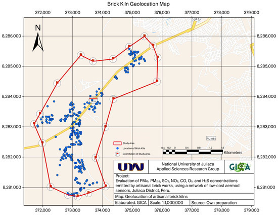
Figure 1.
Locations of Scottish-style artisanal brick kilns in Juliaca City, developed using georeferencing techniques with Global Positioning Systems (GPSs) and Unmanned Aerial Vehicles (UAVs).
2.2. Georeferencing and Emissions Inventory
A georeferenced inventory of artisanal brick kilns was developed through field visits, satellite image analysis, and interviews with producers. More than 300 active kilns were identified for which atmospheric emissions were estimated based on activity intensity and fuel type (sawdust, manure, or used tyres). Emission factors were obtained based on similarity studies, complemented by technical information collected in the study area. Relevant parameters such as chimney height, outlet section dimensions, temperature, and the velocity of emitted gases were recorded for each production unit evaluated, allowing for the calculation of the emission rates of key pollutants, such as particulate matter (PM10 and PM2.5), which were necessary for subsequent modelling.
2.3. Estimation of Atmospheric Emissions
The estimate was based on information collected during the specific inventory conducted in the evaluated geographic area. Emission rates were calculated from emission factors and direct measurements in 5 emitting units in the area under investigation, which were selected considering aspects such as accessibility, representativeness, and reliability. The measurements were obtained using a TESTO portable gas analyser, model T350 (Manufactured by Testo SE & Co. KGaA, Lenzkirch, Germany), with 3 repetitions at intervals of 15 min per point, thus simulating isokinetic sampling, recording mainly concentration, velocity, temperature, and flow parameters. Subsequently, the atmospheric dispersion model AERMOD (American Meteorological Society/Environmental Protection Agency Regulatory Model) [25] was used to process and integrate the collected data to simulate the spatial distribution of pollutants in the receiving areas.
2.3.1. Selection of Emission Factors
Due to the nature of this research, reference emission factors were used for the contaminants PM10 and PM2.5, with values of 29 g/kg and 2.61 g/kg, respectively. For SO2, NO2, and CO, emission rates were estimated, while for O3 and H2S, theoretical factors were applied for modelling under the maximum assumption [36,37].
2.3.2. Emission Rate Calculation
The emission rates for PM10 and PM2.5, as well as O3 and H2S, were calculated by applying the emission factors and activity intensity data obtained through the inventory, using the following equation [38]:
where E is the emission rate (g/s), EF is the emission factor (g/kg), and A is the activity intensity (kg/s).
SO2, NO2, and CO emissions were calculated from direct measurements, and the resulting concentrations were converted to mg/s using the ideal gas equation for converting ppm to mg/m3 under standard dry conditions with 18% oxygen. The concentration and output flow rate of the gases were then multiplied.
2.4. Meteorological Data
Meteorological data were obtained from the National Meteorological and Hydrological Service of Peru (SENAMHI)’s platform [39]. The information gathered was recorded by an automatic meteorological station, identified with the code 472CF72C. The data were recorded on an hourly scale, meaning systematic collection of information at each hour of the day, month, and year, corresponding to the period between 1 January and 31 December 2024. The meteorological variables considered in this study were air temperature, precipitation, relative humidity, wind direction, wind velocity, and cloud cover. The cloud cover data were acquired from the CLIMATE COPERNICUS–ERA-5 platform of the European Centre for Medium-Range Weather Forecasts (ECMWF) [40].
2.5. Model Configuration
Dispersion modelling of atmospheric pollutants was carried out under the guidelines established in the “AERMOD Implementation Guide” provided by the Office of Air Quality Planning and Standards and the Air Quality Assessment Division, Research Triangle Park, under the EPA [41]. The procedure is illustrated in Figure 2.
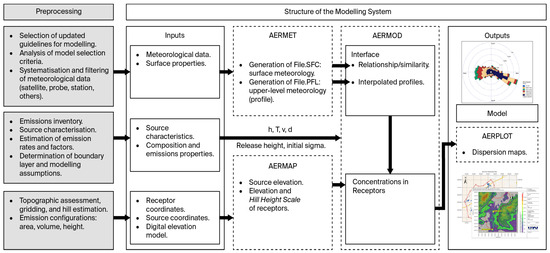
Figure 2.
Structure of the AERMOD pollutant dispersion modelling system [42]. AERMAP computes the elevation of emission sources and the terrain height at receptor locations. AERMET and AERMAP generate output files that serve as inputs for AERMOD, in combination with emission data and source parameters, to simulate pollutant concentration levels (source: adapted from [42]).
2.6. Monitoring with Low-Cost Sensors
Air quality monitoring was carried out continuously over 24 h; the sampling point was located in the brick zone of Juliaca and other parts of the same city. For the determination of PM10 and PM2.5, an optical particle counter was used, which enabled real-time quantification based on the principle of light scattering. To estimate pollutant gases (SO2, NO2, CO, O3 and H2S), electrochemical sensors were used, which operate based on redox-type reactions between the target gases and the sensor electrodes. The precision and measurement ranges of the sensors used are as follows: the evaluation of particulate matter (PM10 and PM2.5) had an accuracy of 0.01 μg/m3 and a range of 0 to 300 μg/m3, while the sensors used for measuring other parameters such as (NO2, CO, O3, and H2S) had an precision of 1 to 15 ppb. In the case of CO, the sensor range corresponds to 0 to 13 ppm, while for NO2, it was 0 to 0.2 ppm, for O3, it was 0 to 0.5 ppm, and for H2S, it was 0 to 3 ppm. The SO2 measurement sensor had an exactness of 1 to 10 ppb and a range of 0 to 0.5 ppm. The air quality monitoring points used in this study are detailed in Table 1.

Table 1.
Spatial distribution of monitoring points for measuring air quality parameters in the study area.
3. Results
3.1. Emissions Inventory
The survey results show that in the study area called “Salida Arequipa”, there are approximately 312 artisanal brick kilns, both operational and non-operational, which are distributed over an area containing 10,558.78 m2 with a perimeter of 15,703 m2, with a seasonality corresponding to the year 2024.
The artisanal Scottish-type kilns have average dimensions of a width of 1.6 m with a raised base, height of 3.70 m, and length of 4.17 m. The kiln crown has an average width of 2.7 m, a length of 3.6 m, and an equivalent diameter of 3.08 m. The mean firing time is 8 h, according to 91% of respondents. A total of 2.16 tons of fuel is used to generate heat to firebrick blocks. The fuel mix is 65% manure, 33% sawdust, and 2% waste tyres. So-called burnings or batches are carried out weekly, with a cumulative duration of 8 h and an activity intensity (A) of 0.075 kg/s, which amounts to burning 0.075 kg of fuel per second.
3.2. Emissions Estimation
3.2.1. Emission Rate Results Using Emission Factors
Emission rates were determined by multiplying emission factors (E) by the activity intensity (A). The activity intensity level is the product of fuel consumption (T) per hour of operation (h), assuming an average fuel consumption of 2.16 T (Table 2).
Table 2.
Emission rates of PM10, PM2.5, and H2S calculated from reference emission factors.
3.2.2. Emission Rate Results from in SITU Measurements
Table 3 presents the results of contaminant gas measurements at the source. These measurements have been corrected for normal conditions and 18% oxygen and expressed in the required units to ensure proper interpretation and analysis. The values reported for each emission source are representative, that is, for each artisanal brick kiln under evaluation.
Table 3.
CO, NOx, and SO2 concentrations determined through direct measurements at the emission outlets of artisanal brick kilns.
Table 4 shows the emission rates of the pollutants SO2, NO2, and CO, determined from the product of the gas concentration measured with the TESTO T350 analyser and its output flow rate. For the O3 concentration, the calculation was based on the assumption of complete stoichiometric conversion of the NO2 precursor, with no reversible reaction in an atmosphere with high radiation and low cloud cover.
Table 4.
Calculated emission rates of SO2, NO2, CO, and O3 (g/s) obtained by electrochemical means under high radiation and low cloud cover conditions during the operation and modelling period.
3.2.3. Measurement of Emission Variables
Table 5 shows the values of the main physical variables recorded during the field measurements, which were used to model the dispersion of contaminants emitted by the brick kilns using the AERMOD View software (version 10.0.0).
Table 5.
Physical environmental variables and parameters (temperature, humidity, wind velocity, etc.) measured in situ with the portable analyser TESTO T350 during the period of operation and modelled in the brick-making zone of Juliaca City.
3.3. Meteorological Analysis
Analysis of meteorological conditions in the study area revealed an average rainfall of 40.5 mm, with the highest rainfall in January and November at 98.7 and 120 mm, respectively. The average temperature was 9.81 °C, with variation from the maximum of 11.66 °C in January to a minimum of 6.22 °C in July. June and July are the coldest months of the year. Relative humidity in the area of interest averaged 54.45%, with a maximum of 65.22% in March and a minimum of 37.50% in July, which is considered the driest period of the year.
Regarding wind velocity, 32.4% of winds were found to occur at velocities between 0.50 and 2.10 m/s, followed by 19.6% in the range of 2.10 to 3.60 m/s, 11.6% between 3.60 and 5.70 m/s, 5.1% between 5.70 and 8.80 m/s, 0.5% between 8.80 and 11.10 m/s, and 0.1% with a velocity greater than 11.10 m/s [Figure 3]. However, 30.3% of the winds were considered calm. Most winds were from the southwest (SE) and northwest (NW), shifting toward the southeast (SE), with velocities ranging from 1.10 to 11.10 m/s and an annual frequency of occurrence greater than 5.8%, as shown in the wind rose diagram above. Cloud cover, expressed in tenths (oktas), was 8/10 during January, March, November, and December. The annual average was 5/10, indicating medium cloud cover during 2024, corresponding to a partly clear sky.
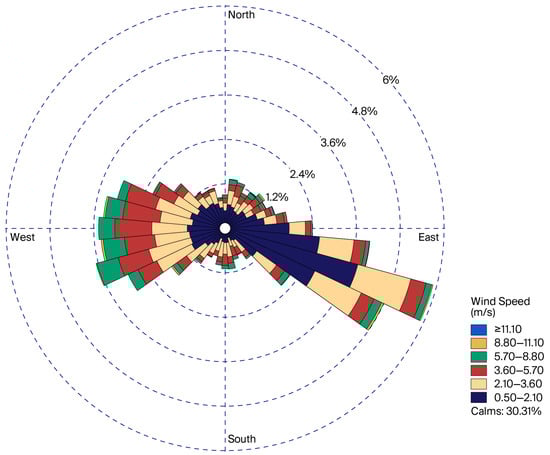
Figure 3.
Wind rose diagram showing the predominant wind velocities and directions recorded in the study area.
3.4. Modelling Contaminant Dispersion
AERMOD [26] was used to analyse each pollutant. The exposure period was 24 h for PM10, PM2.5, SO2, and H2S; 8 h for CO and O2; and 1 h for NO2. Data interpretation considered the maximum permissible concentrations of pollutants according to the Environmental Quality Standards (ECA) for air established by the Ministry of the Environment.
3.4.1. Dispersion of Contaminant PM10
PM10 is dispersed over a distance of 2.64 km from the reference point at UTM coordinates 373,201.00 m east and 8,283,273.00 m south, predominantly towards the southeast. An average distribution of 83.6 m from the emission source was observed. In addition, a maximum concentration of PM10 was identified in the southeast corner of the study area, reaching a value of 562 µg/m3 according to the AERMOD dispersion model [24]. The measurement corresponds to UTM coordinates 373,056.71 m east and 8,280,729.52 m south (Figure 4a).
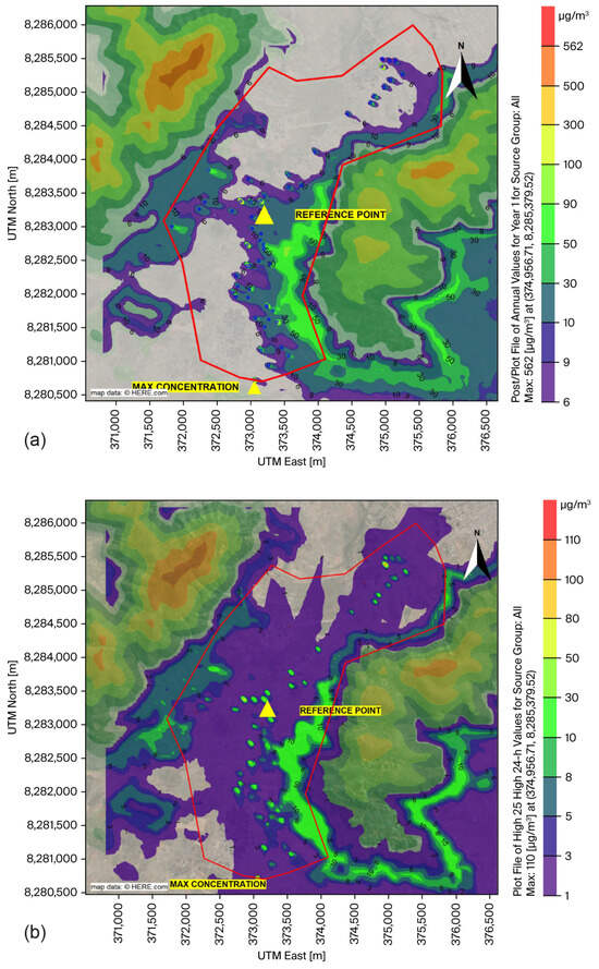
Figure 4.
Dispersion maps of PM10 (a) and PM2.5 (b) derived from emissions from artisanal brick kilns in the study area under typical meteorological conditions in the 2024 dry season. Higher concentrations are observed near the emission sources.
3.4.2. Dispersion of Contaminant PM2.5
Figure 4b illustrates how PM2.5 spread over a distance of 3762 km from the measurement point, located at UTM coordinates 373,201.00 m east and 8,283,273.00 m south, predominantly dispersing towards the northeast and the urban centre of Juliaca City. However, the highest concentration of PM2.5 was located in the southern end of the study area, with the maximum concentration being 110 µg/m3 at UTM coordinates 373,056.71 m east and 8,280,729.52 m, according to AERMOD.
3.4.3. Dispersion of Contaminant SO2
Figure 5a indicates that SO2 propagates a distance of 2.44 km from the monitoring point, between coordinates 373,201.00 m east and 8,283,273.00 m south, highlighting a spread of harmful substances in a southeasterly direction. The highest concentration of SO2 was identified at the southeastern edge of the study area, at coordinates 373,056.32 m east and 8,280,729.89 m south. AERMOD revealed a maximum SO2 concentration of 272 µg/m3.
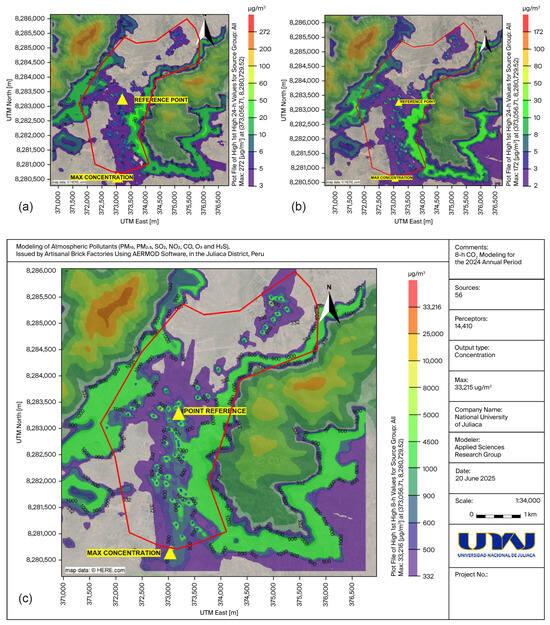
Figure 5.
Dispersion maps of SO2 (a), NOx (b), and CO (c) emitted by artisanal brick kilns in the study area under typical meteorological conditions during the 2024 dry season. Higher concentrations are observed in proximity to the emission sources.
3.4.4. Dispersion of Contaminant NO2
The map in Figure 5b shows the dissemination of NO2 around the emission source in all directions. According to the colour scale, concentrations extended approximately 400 metres around the emission point without following a linear trajectory influenced by wind direction. However, the highest concentration of NO2 was recorded at the southeastern edge of the research area, at coordinates 373,056.71 m east and 8,280,729.52 m south. Modelling results from AERMOD estimated the maximum NO2 concentration at 172 µg/m3.
3.4.5. Dispersion of Contaminant CO
CO disperses in all directions, displaying a radial propagation pattern. The colour spectrum revealed that the average concentration extends approximately 170 metres around the brick kilns, as it does not follow a linear trajectory governed by wind direction. In contrast, the highest concentration of CO was located at the southeastern edge of the geographical focus area, specifically between coordinates 373,056.71 m east and 8,280,729.52 m south. AERMOD showed that the maximum CO concentration was 33,216 µg/m3 (Figure 5c).
3.4.6. Dispersion of Contaminant O3
Figure 6a demonstrates how O3 is scattered irregularly, showing a pattern of propagating in all directions. The colour spectrum evidenced that the average concentration extends up to approximately 180.34 m around the brick kilns, as it does not follow the wind direction. The highest O3 concentration was located at the southeastern edge of the study area, between coordinates 373,056.71 m east and 8,280,729.52 m south. AERMOD evidenced that the maximum O3 concentration was 17.6 µg/m3.
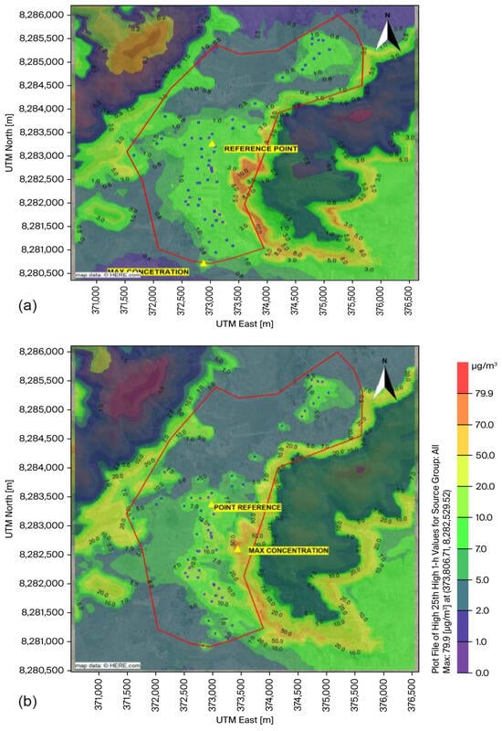
Figure 6.
Dispersion maps of secondary pollutants O3 (a) and H2S (b) emitted by artisanal brick kilns in the study area, assuming complete stoichiometric conversion with no reversible reactions. The highest concentration levels are observed near the emission sources.
3.4.7. Dispersion of Contaminant H2S
The map shows that H2S does not follow a dispersion pattern with a fixed emission source. The spectral range revealed that the average concentration occurs outside the area of focus; according to the figure, the contaminant does not disperse according to the wind direction. Furthermore, AERMOD detected a maximum H2S concentration of 79.94 µg/m3 southeast of the monitoring point, specifically between the coordinates 373,606.71 m east and 8,282,529.52 m south (Figure 6b).
3.5. Concentrations Estimated by AERMOD
Table 6 presents a summary of estimated concentrations for each pollutant using AERMOD. These concentration levels were calculated for a critical scenario over a short-term period. A comparison of this study’s values with the environmental quality standards established in the ECAS Standards is also shown.
Table 6.
Maximum concentrations estimated by AERMOD during periods established according to the ECAs for the pollutants PM10, PM2.5, SO2, NO2, CO, O3, and H2S.
3.6. Monitoring Analysis of Air Quality
Low-cost sensors (LCSs) recorded data with a 5-min time resolution, which were subsequently processed and averaged over hourly intervals for analysis. Regarding particulate matter with a diameter of less than 10 micrometres (PM10), a maximum concentration of 109,928 μg/m3 was recorded at the PM 01 monitoring station, which is the closest to the brick kiln area. The highest values were measured between 3:00 and 7:00 in the morning.
The particulate matter (PM2.5) assessment revealed a maximum value of 87.80 μg/m3 at the PM 01 monitoring point and a minimum value of 33.01 μg/m3, resulting in an average concentration of 51.55 μg/m3 over 24 h at the point closest to the brick-making zone. Similarly, it was observed that the highest concentration was estimated at 4:00 a.m.; on the other hand, the other monitoring points recorded values lower than 29.77 μg/m3.
Concerning nitrogen dioxide (NO2), the maximum hourly concentration reported was 84.13 μg/m3 at PM 01. However, the maximum value monitored was 83.97 μg/m3 at PM 04, while the concentrations lower than 58.19 μg/m3 were detected at PM 02 and PM 03.
Dioxide was recorded at the highest levels at stations PM 01 and PM 04, which are the closest to the monitoring area. The measured levels were 87.8 μg/m3 and 76.36 μg/m3. In contrast, PM 02 and PM 03 presented lower levels at 50.34 and 44.18, respectively.
For carbon monoxide (CO), the maximum concentration was 813.34 μg/m3, which resulted in a high average concentration of 687.10 μg/m3 at the PM 01 monitoring point; similarly, PM 04 recorded 806.67 μg/m3, unlike PM 02 and PM 03, which recorded values data lower than 476.89 μg/m3 and 586.901 μg/m3, calculated over 8 h.
For hydrogen sulphide (H2S), the highest value was recorded at PM 02 at 36.14 μg/m3, followed by 31.29 μg/m3 at PM 04.
Finally, the pollutant ozone (O3) presented a maximum estimated concentration of 108.18 μg/m3 at PM 04. Comparable results were found at PM 01 and PM 03, where values of 93.72 μg/m3 and 106.44 μg/m3 were recorded, respectively.
Figure 7, Figure 8, Figure 9, Figure 10, Figure 11, Figure 12 and Figure 13 present the temporal evolution and variations in the concentrations of particulate matter and pollutant gases monitored by the low-cost sensors (LCSs). Table 7 summarises the maximum values of the parameters analysed and integrates the quantitative information from the corresponding graphical representations.
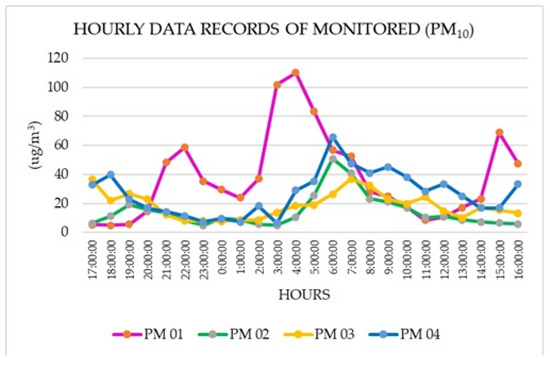
Figure 7.
Hourly record of PM10 particles at monitoring points, recorded using low-cost sensors (LCSs).
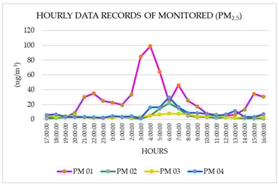
Figure 8.
Hourly record of particulate matter (PM2.5) at monitoring points, recorded using LCSs.
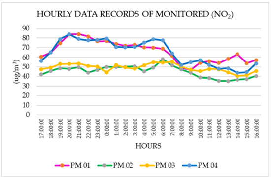
Figure 9.
Hourly record of nitrogen dioxide (NO2) at monitoring points, recorded using LCSs.
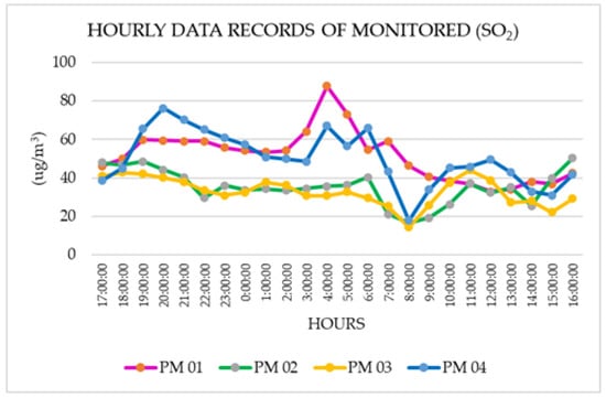
Figure 10.
Hourly record of sulphur dioxide (SO2) at monitoring points, recorded using LCSs.
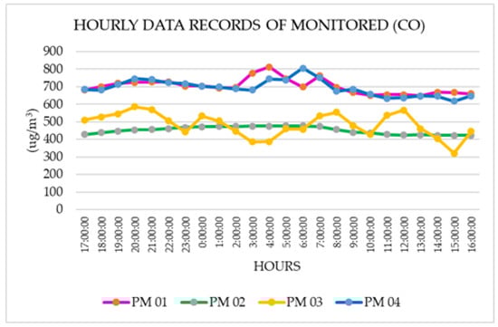
Figure 11.
Hourly record of carbon monoxide (CO) at monitoring points, recorded using LCSs.
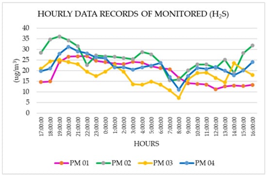
Figure 12.
Hourly record of hydrogen sulphide (H2S) at monitoring points, recorded using LCSs.
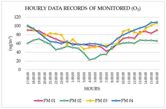
Figure 13.
Hourly record of ozone (O3) at monitoring points, obtained using low-cost sensors (LCSs).
Table 7.
Comparison of concentrations obtained from air quality monitoring with the Environmental Quality Standard (AQS).
The values in Table 7 show the monitoring results, which objectively demonstrate that the maximum concentrations recorded are below the parameters established in the Environmental Quality Standard (ECA) for air.
3.7. Data Comparison
The data derived from the emissions inventory and the modelling of pollutant dispersion from the point sources (brick kilns) were compared with the maximum concentrations recorded by the low-cost sensors (LCSs). The results of this comparison are presented in Table 8.
Table 8.
Relationship of maximum concentrations obtained from air quality monitoring with data from pollutant dispersion modelling.
Based on a comprehensive analysis of data collected through air quality monitoring with low-cost sensors and emission estimation procedures, this study assessed the relative contribution of emissions from brick kilns to the overall concentrations of the targeted atmospheric pollutants.
4. Discussion
This study aimed to interpret the quantified concentrations and spatial distribution patterns of air pollutants emitted by artisanal brick kilns in Juliaca City, based on dispersion modelling using AERMOD and obtained data from the low-cost sensor network. The analysis sought to contextualise these findings in relation to the existing literature on emissions from informal or small-scale industrial sources, evaluate the performance and limitations of the methodologies employed—especially based on local conditions—and identify implications for public health and environmental management. Although the research introduces a novel georeferenced emissions inventory and utilises robust modelling tools, certain limitations, such as the use of estimated emission factors, uncertainties in sensor calibration, and temporal variability in kiln operations, may influence the accuracy and generalizability of the results.
4.1. Impact of Emissions from Artisanal Brick Kilns on Air Quality and Public Health
The artisanal brick kilns in Juliaca City are a significant source of atmospheric pollution, with emissions frequently exceeding the limits recommended by the World Health Organization (WHO). Recent studies have shown that emissions from these kilns contain high concentrations of fine (PM2.5) and ultrafine particles, which pose serious risks to respiratory and cardiovascular health [43]. A particularly concerning aspect is the burning of non-conventional fuels, such as used tyres and plastic waste. The combustion of these fuels significantly increases the emission of volatile organic compounds and highly toxic heavy metals [44].
Constant exposure to these contaminants has been associated with an increased incidence of chronic obstructive pulmonary disease (COPD) and lung cancer among populations living near brick-making areas [45]. In the case of Juliaca, the situation is further exacerbated by specific geographic and climatic factors. The high altitude (3824 m above sea level) and low average temperatures (9.81 °C) favour the accumulation of pollutants near emission sources, thereby increasing exposure for the local population [46]. Moreover, the predominant wind direction (from southwest to northwest) transports pollutants towards densely populated areas, which could explain the high prevalence of respiratory diseases reported in these regions [47].
4.2. Modelling of Atmospheric Pollutants Using AERMOD
The modelling conducted using AERMOD enabled the identification of clear spatial patterns in pollutant dispersion, with higher concentrations observed southeast from the emission sources. However, significant discrepancies were detected between the modelled and measured concentrations, particularly in the case of CO (33,216 µg/m3 against 687.1 µg/m3). These differences could be attributed to inherent limitations of the model in adequately representing (1) non-point source fugitive emissions, (2) turbulence effects over complex terrain, and (3) temporal variations in emission rates [48].
Recent studies suggest that incorporating artificial intelligence-based techniques could significantly improve the accuracy of traditional dispersion models [49]. In particular, machine learning algorithms have demonstrated the ability to capture non-linear relationships between meteorological variables and dispersion patterns, reducing prediction error by up to 30% [50]. Nevertheless, using these advanced methods in contexts such as Juliaca requires careful consideration of the limited availability of high-quality input data.
This research was structured into clearly defined and distinct stages, which facilitated the achievement of its objectives. The first stage involved data preprocessing, which included an analysis of the model and its characteristics, leading to a search for highly reliable meteorological data, in accordance with the guidelines established by the United States Environmental Protection Agency (EPA) and the American Meteorological Society (AMS) [26]. Meteorological data were obtained from the platform of the Peruvian National Service of Meteorology and Hydrology (SENAMHI) [39]. Data collection was conducted at an automatic meteorological station with the code 472CF72C, from which systematic hourly records were obtained for the period from 1 January to 31 December 2024.
Cloud cover data were obtained from the CLIMATE COPERNICUS–ERA-5 platform of the European Centre for Medium-Range Weather Forecasts (ECMWF) [40], which provided relevant information for the determination of the boundary layer and application of the model. The prevailing winds were from the southwest and northwest (SW-NW), moving in a southeast (SE) direction, with velocities between 1.10 and 11.10 m/s and an annual frequency of appearance greater than 5.8%. This information is provided in the wind rose diagram and distribution. Furthermore, a maximum of 32.4% of winds had velocities of 0.50–2.10 m/s, while 19.6% had velocities of 2.10–3.60 m/s, 11.6% had velocities of 3.60–5.70 m/s, 5.1% had velocities of 5.70–8.80 m/s, 0.5% had velocities of 8.80–11.10 m/s, and 0.1% had a velocity greater than 11.10 m/s. However, 30.3% of winds were calm.
In the second stage, an emissions inventory was conducted, enabling the georeferencing and identification of 312 artisanal brick producers distributed across an area of 10,558.78 m2. This distribution is consistent with the records of the Ministry of Production (PRODUCE) and the San Román Provincial Municipality (MPSR) [30,32]. This inventory enabled the characterisation of kiln features, including their dimensions (1.6 × 4.7 m and 3.70 m in height), crown measurements (average of 2.7 × 3.6 m), and equivalent diameter (3.08 m). Operational conditions were also determined, including the type of fuel used—65% manure, 33% sawdust, and 2% waste tires—for an average firing time of 8 h and a total fuel mixture of 2.16 tons. These values are consistent with those reported by Vera [36], who documented 7.18 tons used over a 24-h period.
The estimated concentration of pollutants in the exhaust gases emitted by brick kilns in Juliaca City reached 11,679.87 mg/m3N of CO, 141.49 mg/m3N of NOx, and 236.67 mg/m3N of SO2. CO is the most abundant pollutant, exceeding the Maximum Permitted Limit (MPL) of the Peruvian environmental standard by 85%. In this regard, Vera [36] reported a maximum concentration of 133.12 µg/m3 of PM10, indicating that the high concentrations are due to meteorological and geographical factors specific to the location. Pozo [51] reported 121 µg/m3 of PM2.5, stating that the concentration is influenced by the prevailing winds and atmospheric stability. On the other hand [52], Halanocca showed a maximum concentration of 24 µg/m3 of SO2 in brickyard areas. The significant difference in results is likely due to the type of fuel used to fire the bricks.
The contributions of the pollutants emitted by artisanal brick kilns in Juliaca City were estimated using the AERMOD dispersion model. The results indicated maximum concentrations of 562 µg/m3 for PM10, 110 µg/m3 for PM2.5, 272 µg/m3 for SO2, 172 µg/m3 for NO2, 33,216 µg/m3 for CO, 17.6 µg/m3 for O3, and 79.9 µg/m3 for H2S. Among these pollutants, only the concentrations of NO2, O3, and H2S were within the limits established by the Environmental Quality Standards (ECA). Additionally, the emission rates, calculated from both emission factors and direct measurements, of the brick kilns were estimated at 29, 0.190, 0.21, 0.15, 12.84, 0.157, and 0.113 g/s for PM10, PM2.5, SO2, NO2, CO, O3, and H2S, respectively. In this regard, Halanocca [52] reported a maximum SO2 concentration of 24 µg/m3 in brick-manufacturing zones. The results reveal a notable difference, which is likely attributable to the type of fuel used by the brick producers during the firing process. Similarly, Neyra and Dalens et al. [53,54] reported CO concentrations of 1120.2 µg/m3 and 4939 µg/m3, respectively. With respect to the estimated concentrations of H2S and O3, values of 17.6 µg/m3 and 79.9 µg/m3 were observed, respectively.
4.3. Monitoring with Low-Cost Sensors: Advantages and Limitations
The low-cost sensor network implemented in this study proved to be a valuable tool for real-time air quality monitoring. The electrochemical sensors used showed good correlation (R2 > 0.85) with reference instruments for the measurement of SO2 and NO2 [55]. Nonetheless, meaningful challenges were identified in the measurement of particulate matter, as the optical sensors exhibited considerable variability (±25%) under conditions of high relative humidity [56].
Recent experiences in Latin America [57] suggest that the performance of these networks can be enhanced through periodic calibration against reference instruments, the implementation of correction algorithms that account for environmental conditions, and optimised network design based on emission sources and wind circulation patterns.
4.4. Limitations
Developing countries face deficiencies in the availability of reliable data for meteorological data processing. In this study, modelling assumed the simultaneous operation of 56 kilns, which leads to substantial differences between the estimated concentrations and those measured by low-cost sensors, as observed in the case of CO.
Despite their limitations, the combined use of low-cost sensors with dispersion models is a cost-effective solution for environmental monitoring in resource-limited regions. This hybrid approach has proven particularly useful for identifying pollution hotspots and evaluating the effectiveness of control measures [58].
5. Conclusions
This study highlights the effectiveness of combining Geographic Information Systems (GISs), AERMOD modelling, and low-cost sensors (LCSs) to evaluate atmospheric emissions and their spread in urban areas bustling with industrial activity. By examining 312 brick kilns in Juliaca, we were able to conduct a thorough environmental assessment that has direct implications for managing local air quality.
One of the standout contributions of this research is the creation of dispersion maps for crucial pollutants like PM10, PM2.5, SO2, NO2, CO, H2S, and O3. These maps pinpoint environmental risk zones and can help shape targeted public policies for mitigation. Additionally, the blend of modelling and on-the-ground monitoring offers a replicable strategy for similar contexts with informal industries and limited environmental resources.
Nevertheless, we need to recognize some methodological limitations, such as the use of average meteorological data and low-cost sensors, which tend to have more uncertainty compared to high-grade instruments. These aspects could influence the accuracy of our estimates and should be taken into account in future studies.
The pollutant distribution estimated using the AERMOD dispersion model allowed for the calculation of maximum concentrations of 562 μg/m3 (PM10), 110 μg/m3 (PM2.5), 272 μg/m3 (SO2), 172 μg/m3 (NO2), 33,216 μg/m3 (CO), 17.6 (O3), and 79.9 H2S with corresponding maximum dispersion distances of 0.0836, 3.762, 2.44, 0.4, and 0.17 Km, respectively. Air quality monitoring using low-cost sensors (LCSs)—which involved the measurement of PM10 and PM2.5 via an optical particle counter and the measurement of SO2, NO2, and CO through electrochemical sensors—enabled the determination of daily averages of 28.14 μg/m3 (PM10), 26.96 μg/m3 (PM2.5), 51.55 μg/m3 (SO2), and 86.86 μg/m3 (O3). For CO, an 8-h average concentration of 687.1 μg/m3 was recorded. The maximum observed concentrations for NO2 and H2S were 84.13 μg/m3 and 26.8 μg/m3.
To build on this approach, it would be beneficial to implement long-term monitoring campaigns, validate findings with certified stations, and explore the impacts on public health. This study lays strong technical and methodological groundwork to enhance environmental monitoring in mid-sized cities throughout Latin America.
Author Contributions
Conceptualization, J.L.P.-T., K.F.Q.-M., R.C.-S. and M.L.S.-H.; methodology, J.L.P.-T., K.F.Q.-M., R.C.-S. and M.L.S.-H.; software, J.L.P.-T., K.F.Q.-M., R.C.-S. and M.L.S.-H.; validation, J.L.P.-T., E.H.-H., M.E.H.-F., K.F.Q.-M., R.C.-S. and M.L.S.-H.; formal analysis, J.L.P.-T., E.H.-H., M.E.H.-F., K.F.Q.-M., R.C.-S. and M.L.S.-H.; investigation, J.L.P.-T., E.H.-H., M.E.H.-F., K.F.Q.-M., R.C.-S., M.L.S.-H., D.E.M.-V. and C.A.C.-F.; resources, J.L.P.-T., R.C.-S. and M.L.S.-H.; data curation, J.L.P.-T., M.E.H.-F., K.F.Q.-M., R.C.-S. and M.L.S.-H.; writing—original draft preparation, J.L.P.-T., E.H.-H., M.E.H.-F., K.F.Q.-M., R.C.-S., M.L.S.-H., C.A.C.-F. and D.L.-C.; writing—review and editing, J.L.P.-T. and D.L.-C.; visualization, J.L.P.-T., E.H.-H., M.E.H.-F., K.F.Q.-M., R.C.-S., M.L.S.-H. and D.L.-C.; supervision, J.L.P.-T.; project administration, J.L.P.-T. and E.H.-H.; funding acquisition, J.L.P.-T., R.C.-S., M.L.S.-H., D.E.M.-V. and E.H.-H. All authors have read and agreed to the published version of the manuscript.
Funding
This research received funding from Universidad Nacional de Juliaca CANON funds. With contract number 002-2023-VPIN-CCO-UNAJ.
Data Availability Statement
The data presented in this study are available upon request from the corresponding author.
Conflicts of Interest
The authors declare no conflicts of interest.
Abbreviations
The following abbreviations are used in this manuscript:
| UNAJ | National University of Juliaca |
| GISs | Geographic Information Systems |
| LCS | Low-Cost Sensor |
| AQS | Air Quality Standards |
| EPA | Environmental Protection Agency |
| UTM | Universal Transverse Mercator |
| WHO | World Health Organization |
| SENAMHI | Peruvian National Service of Meteorology and Hydrology |
| AMS | American Meteorological Society |
| ECMWF | European Centre for Medium-Range Weather Forecasts |
| PRODUCE | Ministry of Production |
| MPSR | San Román Provincial Municipality |
| MPL | Maximum Permitted Limit |
References
- Hassan Bhat, T.; Jiawen, G.; Farzaneh, H. Air Pollution Health Risk Assessment (AP-HRA), Principles and Applications. Int. J. Environ. Res. Public Health 2021, 18, 1935. [Google Scholar] [CrossRef]
- Huang, X. The Impact of PM10 and Other Airborne Particulate Matter on the Cardiopulmonary and Respiratory Systems of Sports Personnel under Atmospheric Exposure. Atmosphere 2023, 14, 1697. [Google Scholar] [CrossRef]
- Mannucci, P.M.; Franchini, M. Health Effects of Ambient Air Pollution in Developing Countries. Int. J. Environ. Res. Public Health 2017, 14, 1048. [Google Scholar] [CrossRef]
- World Health Organization. Air Quality and Health. Available online: https://www.who.int/health-topics/air-pollution#tab=tab_1 (accessed on 14 April 2025).
- Künzli, N.; Perez, L.; Rapp, R. Air Pollution and Health: A European Respiratory Society Booklet; European Respiratory Society: Lausanne, Switzerland, 2010; ISBN 978-1-84984-008-8. [Google Scholar]
- Ubilla, C.; Yohannessen, K. Outdoor Air Pollution Respiratory Health Effects in Children. Rev. Med. Clin. Las Condes 2017, 28, 111–118. [Google Scholar] [CrossRef]
- Omidvarborna, H.; Baawain, M.; Albo-Mamun, A. Ambient Air Quality and Exposure Assessment Study of the Gulf Cooperation Council Countries: A Critical Review. Sci. Total Environ. 2018, 636, 437–448. [Google Scholar] [CrossRef]
- Afzali, A.; Rashid, M.; Afzali, M.; Younesi, V. Prediction of Air Pollutants Concentrations from Multiple Sources Using AERMOD Coupled with WRF Prognostic Model. J. Clean. Prod. 2017, 166, 1216–1225. [Google Scholar] [CrossRef]
- Amoatey, P.; Omidvarborna, H.; Baawain, M.S.; Al-Mamun, A. Emissions and Exposure Assessments of SOX, NOX, PM10/2.5 and Trace Metals from Oil Industries: A Review Study (2000–2018). Process Saf. Environ. Prot. 2019, 123, 215–228. [Google Scholar] [CrossRef]
- Roy, A.; Bhattacharya, T.; Kumari, M. Air Pollution Tolerance, Metal Accumulation and Dust Capturing Capacity of Common Tropical Trees in Commercial and Industrial Sites. Sci. Total Environ. 2020, 722, 137622. [Google Scholar] [CrossRef]
- Fischer, P.H.; Marra, M.; Ameling, C.B.; Velders, G.J.M.; Hoogerbrugge, R.; de Vries, W.; Wesseling, J.; Janssen, N.A.H.; Houthuijs, D. Particulate Air Pollution from Different Sources and Mortality in 7.5 Million Adults—The Dutch Environmental Longitudinal Study (DUELS). Sci. Total Environ. 2020, 705, 135778. [Google Scholar] [CrossRef]
- de Miguel-Diez, J.; Blasco-Esquivias, I.; Rodriguez-Matute, C.; Bedate-Diaz, P.; Lopez-Reyes, R.; Fernandez-Capitan, C.; Garcia-Fuika, S.; Lobo-Beristain, J.L.; Garcia-Lozaga, A.; Quezada, C.A.; et al. Correlation between Short-Term Air Pollution Exposure and Unprovoked Lung Embolism: Prospective Observational Study (Contamina-TEP Group). Thromb. Res. 2020, 192, 134–140. [Google Scholar] [CrossRef]
- Biswas, N.; Ghosh, A.; Mitra, S.; Majumdar, G. Environmental issues associated with mining and minerals processing. Compr. Mater. Process. 2024, 8, 77–86. [Google Scholar] [CrossRef]
- Hossin, M.A.; Haque, A.; Saha, O.; Islam, R.; Shimin, T.I. Un análisis espaciotemporal de los contaminantes del aire durante y después de COVID-19: Un estudio de caso de la división de Dhaka utilizando Google Earth Engine. DYSONA-Apl. Ciencia. 2025, 6, 411–421. [Google Scholar] [CrossRef]
- Jion, M.M.M.F.; Jannat, J.N.; Mia, Y.; Ali, A.; Islam, S.; Ibrahim, S.M.; Pal, S.C.; Islam, A.; Sarker, A.; Malafaia, G.; et al. A critical review and prospect of NO2 and SO2 pollution over Asia: Hotspots, trends, and sources. Sci. Total Environ. 2023, 876, 162851. [Google Scholar] [CrossRef]
- López Juvinao, D.D.; Torres Ustate, L.M.; Moya Camacho, F.O. Tecnologías, Procesos y Problemática Ambiental en la Minería de Arcilla. Inv. Innov. Ing. 2020, 8, 20–43. [Google Scholar] [CrossRef]
- Darain, K.M.U.; Jumaat, M.Z.; Islam, A.B.M.S.; Obaydullah, M.; Iqbal, A.; Adham, M.I.; Rahman, M.M. Energy Efficient Brick Kilns for Sustainable Environment. Desalin. Water Treat. 2016, 57, 105–114. [Google Scholar] [CrossRef]
- Turpo Turpo, V.L.; Lipa Soncco, L.D. Evaluación de las Propiedades Físico-Mecánicas de un Adoquín Adicionando Cenizas de Ladrilleras Artesanales-Juliaca 2021. Bachelor’s Thesis, Universidad Peruana Unión, Juliaca, Peru, 2021. [Google Scholar]
- World Health Organization. Air Quality Guidelines: Global Update 2021. Available online: https://www.who.int/publications/i/item/9789240034228 (accessed on 14 April 2025).
- Chen, Y.; Du, W.; Zhuo, S.; Liu, W.; Liu, Y.; Shen, G.; Wu, S.; Li, J.; Zhou, B.; Wang, G.; et al. Stack and Fugitive Emissions of Major Air Pollutants from Typical Brick Kilns in China. Environ. Pollut. 2017, 224, 421–429. [Google Scholar] [CrossRef]
- United States Environmental Protection Agency (EPA). Health and Environmental Effects of Air Pollutants. Available online: https://www.epa.gov/criteria-air-pollutants (accessed on 14 April 2025).
- Abidin, A.U.; Munawaroh, A.L.; Rosinta, A.; Sulistiyani, A.T.; Ardianta, I.; Iresha, F.M. Environmental Health Risks and Impacts of PM2.5 Exposure on Human Health in Residential Areas, Bantul, Yogyakarta, Indonesia. Toxicol. Rep. 2025, 14, 101949. [Google Scholar] [CrossRef]
- Ulloa Ninahuamán, J.; Alvarez-Tolentino, D.; Peña Rojas, A.; Suarez-Salas, L. Sensores de bajo costo en la caracterización de partículas finas (PM2.5) de una ciudad altoandina. Rev. Investig. Altoandinas 2022, 24, 199–207. [Google Scholar] [CrossRef]
- Rood, A. Performance Evaluation of AERMOD, CALPUFF, and Legacy Air Dispersion Models Using the Winter Validation Tracer Study Dataset. Atmos. Environ. 2014, 89, 707–720. [Google Scholar] [CrossRef]
- Van Leuken, J.P.G.; Swart, A.N.; Havelaar, A.H.; Van Pul, A.; Van der Hoek, W.; Heederik, D. Atmospheric Dispersion Modelling of Bioaerosols That Are Pathogenic to Humans and Livestock—A Review to Inform Risk Assessment Studies. Microb. Risk Anal. 2016, 1, 19–39. [Google Scholar] [CrossRef]
- Gibson, M.D.; Kundu, S.; Satish, M. Dispersion Model Evaluation of PM2.5, NOX, and SO2 from Point and Major Line Sources in Nova Scotia, Canada Using AERMOD Gaussian Plume Air Dispersion Model. Atmos. Pollut. Res. 2013, 4, 157–167. [Google Scholar] [CrossRef]
- Askariyeh, M.; Kota, S.; Vallamsundar, S.; Zietsman, J.; Ying, Q. AERMOD for Near-Road Pollutant Dispersion: Evaluation of Model Performance with Different Emission Source Representations and Low Wind Options. Transp. Res. Part D Transp. Environ. 2017, 57, 392–402. [Google Scholar] [CrossRef]
- Carbonell, L.; Sanchez Gacita, M.; Rivero Oliva, J.; Garea, L.; Rivero, N.; Meneses, E. Methodological Guide for Implementation of the AERMOD System with Incomplete Local Data. Atmos. Pollut. Res. 2010, 1, 102–111. [Google Scholar] [CrossRef]
- Melo, A.; Santos, J.M.; Mavroidis, I.; Neyval, J. Modelling of Odour Dispersion Around a Pig Farm Building Complex Using AERMOD and CALPUFF: Comparison with Wind Tunnel Results. Build. Environ. 2012, 56, 8–20. [Google Scholar] [CrossRef]
- Rubio, J.J.; Hernández-Aguilar, J.A.; Ávila-Camacho, F.J.; Stein-Carrillo, J.M.; Meléndez-Ramírez, A. Sistema Sensor para el Monitoreo Ambiental Basado en Redes Neuronales. Ing. Investig. Tecnol. 2016, 17, 211–222. [Google Scholar] [CrossRef]
- de Aire Limpio, P.R.; de la Producción, M. Estudio Diagnóstico Sobre las Ladrilleras Artesanales en el Perú; Swisscontact: Lima, Peru, 2006; Available online: https://www.produce.gob.pe (accessed on 14 April 2025).
- Soriano Giraldo, C. Diagnóstico Nacional del Sector Ladrillero Artesanal; Mercadeando S.A.: Piura, Peru, 2012; Available online: https://www.munichulucanas.gob.pe/jdownloads/documentos_de_gestion/diagnostico_ladrilleras_morropon.pdf (accessed on 14 April 2025).
- Román, M.P.S.; de Vivienda, M.; Saneamiento, C.Y. Plan de Desarrollo Urbano de la Ciudad de Juliaca 2016–2025; Municipalidad Provincial San Román: San Román, Puno, Peru, 2015; Available online: https://cdn.www.gob.pe/uploads/document/file/5641653/4997450-iii-1-sub-sistema-fisico-biotico.pdf?v=1704496400 (accessed on 15 April 2025).
- Aucapuri Figueroa, J.; Caviedes Villa, Y.; Chura Quispe, G.E.; Zanabria Acuña, A. Planeamiento Estratégico del Distrito de Juliaca. Master’s Thesis, Pontificia Universidad Católica del Perú, Lima, Peru, 2018. [Google Scholar]
- Giarra, A.; Riccio, A.; Chianese, E.; Annetta, M.; Toscanesi, M.; Trifuoggi, M. Mecanismos de transporte y dinámica de contaminantes que influyen en los niveles de PM10 en una región densamente urbanizada e industrializada cerca de Nápoles, sur de Italia: Un análisis del tiempo de residencia. Atmósfera 2025, 16, 393. [Google Scholar] [CrossRef]
- Vera, M. Modelamiento de la dispersión de PM10 de las ladrilleras del distrito de San Jerónimo Cusco. Rev. Boliv. Quím. 2023, 40, 5–12. [Google Scholar] [CrossRef]
- CAEM; CCAC; Herrera, P.A.; Rodríguez, A.L.; Salgado, F.A.; Ruiz, B.; Beltrán, D.F. Determinación de Factores de Emisión que Servirán como Insumo para la Herramienta LEAP-IBC; Corporación Ambiental Empresarial (CAEM), Coalición de Clima y Aire Limpio (CCAC), Ministerio de Ambiente y Desarrollo Sostenible: Bogotá, Colombia, 2020; Available online: https://cdn.www.gob.pe/uploads/document/file/5641653/4997450-iii-1-sub-s (accessed on 14 April 2025).
- U.S. Environmental Protection Agency (EPA). AP-42: Compilation of Air Pollutant Emission Factors from Stationary Sources; 2025 ed.; EPA: Washington, DC, USA, 2025. Available online: https://www.epa.gov/air-emissions-factors-and-quantification/ap-42-compilation-air-emissions-factors-stationary-sources (accessed on 2 July 2025).
- Servicio Nacional de Meteorología e Hidrología del Perú (SENAMHI). Datos Meteorológicos Diarios del Año 2024—Estación Juliaca [472CF72C]. 2025. Available online: https://www.senamhi.gob.pe/?p=estaciones (accessed on 2 July 2025).
- Copernicus Climate Change Service (C3S). ERA5: Hourly Data on Single Levels from 1940 to Present. 2023. Climate Data Store (CDS). Available online: https://cds.climate.copernicus.eu/datasets/reanalysis-era5-single-levels?tab=overview (accessed on 1 July 2025).
- United States Environmental Protection Agency (US EPA). Guideline on Air Quality Models; Enhancements to the AERMOD Dispersion Modeling System. 2024. Available online: www.epa.gov/scram/2024-appendix-w- (accessed on 14 April 2025).
- Cimorelli, A.J.; Perry, S.G.; Venkatram, A.; Weil, J.C.; Paine, R.J.; Wilson, R.B.; Lee, R.F.; Peters, W.D.; Brode, R.W.; Paumier, J.O. AERMOD: Description of Model Formulation; EPA-454/R-03-004; U.S. Environmental Protection Agency, Office of Air Quality Planning and Standards: Research Triangle Park, NC, USA, 2004. Available online: https://www.epa.gov/scram/air-quality-dispersion-modeling-alternative-models (accessed on 24 April 2025).
- Nicolaou, L.; Sylvies, F.; Veloso, I.; Lord, K.; Chandyo, R.K.; Sharma, A.K.; Shrestha, L.P.; Parker, D.L.; Thygerson, S.M.; DeCarlo, P.F.; et al. Brick Kiln Pollution and Its Impact on Health: A Systematic Review and Meta-Analysis. Environ. Res. 2024, 257, 119220. [Google Scholar] [CrossRef] [PubMed]
- Berumen-Rodríguez, A.A.; Pérez-Vázquez, F.J.; Díaz-Barriga, F.; Márquez-Mireles, L.E.; Flores-Ramírez, R. Revisión del Impacto del Sector Ladrillero sobre el Ambiente y la Salud Humana en México. Salud Pública Méx. 2021, 63, 100–108. [Google Scholar] [CrossRef]
- González, N.; Valero, A.; Rodríguez, Y.; Rodríguez, J.; Vargas, L. Síntomas Respiratorios en Trabajadores de Ladrilleras de Tunja, Boyacá, Colombia. Med. Int. Méx. 2021, 37, 704–715. [Google Scholar] [CrossRef]
- Mardoñez, V.; Pandolfi, M.; Borlaza, L.J.S.; Jaffrezo, J.-L.; Alastuey, A.; Besombes, J.-L.; Moreno, R.I.; Perez, N.; Močnik, G.; Ginot, P.; et al. Source Apportionment Study on Particulate Air Pollution in Two High-Altitude Bolivian Cities: La Paz and El Alto. Atmos. Chem. Phys. 2023, 23, 10325–10347. [Google Scholar] [CrossRef]
- Jiang, J.; Jin, A. Study on the Dispersion Law of Typical Pollutants in Winter by Complex Geographic Environment Based on the Coupling of GIS and CFD—A Case Study of the Urumqi Region. Appl. Sci. 2025, 15, 2469. [Google Scholar] [CrossRef]
- Venkatram, A.; Brode, R.; Cimorelli, A.; Lee, R.; Paine, R.; Perry, S.; Peters, W.; Weil, J.; Wilson, R. A Complex Terrain Dispersion Model for Regulatory Applications. Atmos. Environ. 2001, 35, 4211–4221. [Google Scholar] [CrossRef]
- Kalantari, E.; Gholami, H.; Malakooti, H.; Nafarzadegan, A.R.; Moosavi, V. Machine Learning for Air Quality Index (AQI) Forecasting: Shallow Learning or Deep Learning? Environ. Sci. Pollut. Res. 2024, 31, 62962–62982. [Google Scholar] [CrossRef]
- Maffi, J.M.; Estenoz, D.A. Predicting Phase Inversion in Agitated Dispersions with Machine Learning Algorithms. Chem. Eng. Commun. 2020, 208, 1757–1774. [Google Scholar] [CrossRef]
- Suclupe, P.; Antonio, L. Identificación de Impactos Ambientales Significativos En La Industria Ladrillera Utilizando Un Modelo de Simulación Dinámica. TZHOECOEN 2018, 10, 593–609. [Google Scholar] [CrossRef]
- Halanocca Quispe, Y.; Huamán Valencia, R.S. Impacto Ambiental Generado por el Sector Ladrillero en el Distrito de San Jerónino-Cusco. Bachelor’s Thesis, Universidad Nacional de San Antonio Abad del Cusco, Cusco, Peru, 2015. [Google Scholar]
- Inga, H.; Rosario, N. Modelamiento de la dispersión de gases utilizando el Aermod versión 8.9 y su relación con los parámetros meteorológicos del Centro Poblado Santa Maria de Huachipa, 2019. Bachelor’s Thesis, Universidad Cesar Vallejo, Trujillo, Peru, 2019. Available online: https://hdl.handle.net/20.500.12692/40527 (accessed on 10 September 2025).
- Dalens Rojas, Z.E.; Macedo Gallegos, T. Evaluación de la Calidad del aire por Emisiones de CO, PM2. 5, PM10 Generado por la Industria Ladrillera en Cusco. Bachelor’s Thesis, Universidad Cesar Vallejo, Lima, Peru, 2022. [Google Scholar]
- Chojer, H.; Branco, P.T.B.S.; Martins, F.G.; Sousa, S.I.V. A Novel Low-Cost Sensors System for Real-Time Multipollutant Indoor Air Quality Monitoring: Development and Performance. Build. Environ. 2024, 266, 112055. [Google Scholar] [CrossRef]
- Jayaratne, R.; Liu, X.; Thai, P.; Dunbabin, M.; Morawska, L. La Influencia de la Humedad en el Rendimiento de un Sensor de Masa de Partículas de Aire de Bajo Costo y el Efecto de la Niebla Atmosférica. Atmos. Meas. Tech. 2018, 11, 4883–4890. [Google Scholar] [CrossRef]
- Vázquez-Torres, C.E.; Quijano-Cetina, R.G.; Sánchez-Domínguez, I.; Ali, B. Potential of a Low-Cost System for Measuring Indoor Environmental Quality in Latin American Extreme Climates Towards Energy Equity. Habitat Sustentable 2024, 14, 76–85. [Google Scholar] [CrossRef]
- McFarlane, C.; Raheja, G.; Malings, C.; Appoh, E.; Hughes, A.; Westervelt, D. Application of Gaussian Mixture Regression for the Correction of Low-Cost PM2.5 Monitoring Data in Accra, Ghana. ACS Earth Space Chem. 2021, 5, 2268–2279. [Google Scholar] [CrossRef]
Disclaimer/Publisher’s Note: The statements, opinions and data contained in all publications are solely those of the individual author(s) and contributor(s) and not of MDPI and/or the editor(s). MDPI and/or the editor(s) disclaim responsibility for any injury to people or property resulting from any ideas, methods, instructions or products referred to in the content. |
© 2025 by the authors. Licensee MDPI, Basel, Switzerland. This article is an open access article distributed under the terms and conditions of the Creative Commons Attribution (CC BY) license (https://creativecommons.org/licenses/by/4.0/).