Experimental and Molecular Dynamics Simulation of Interfacial Tension Measurements in CO₂–Brine/Oil Systems: A Literature Review

Abstract

Carbon dioxide (CO₂), a major greenhouse gas, contributes significantly to global warming and environmental degradation. Carbon Capture, Utilization, and Storage (CCUS) is a promising strategy to mitigate atmospheric CO₂ levels. One widely applied utilization approach involves injecting captured CO₂ into depleted oil reservoirs to enhance oil recovery—a technique known as CO₂-Enhanced Oil Recovery (CO₂-EOR). The effectiveness of CO₂-EOR largely depends on complex rock–fluid interactions, including mass transfer, wettability alteration, capillary pressure, and interfacial tension (IFT). Various factors, such as the presence of asphaltenes, salinity, pressure, temperature, and rock type, influence these interactions. This review explores the impact of these parameters on the IFT between CO₂ and oil/water systems, drawing on findings from both experimental studies and molecular dynamics (MD) simulations. The literature indicates that increased temperature, reduced pressure, lower salinity, and the presence of asphaltenes tend to reduce IFT at the oil–water interface. Similarly, elevated temperature and pressure, along with asphaltene content, also lower the surface tension between CO₂ and oil. Most MD simulations employ synthetic oil mixtures of various alkanes and use tools such as LAMMPS and GROMACS. Experimentally, the pendant drop method is most commonly used with crude oil and brine samples. Future research employing actual reservoir fluids and alternative measurement techniques may yield more accurate and representative IFT data, further advancing the application of CO₂-EOR.

1. Introduction

The combustion of fossil fuels has contributed to higher levels of CO₂, a major driver of climate change, and increased ocean acidity. Carbon capture and storage in deep saline aquifers and depleted oil and gas reservoirs are effective methods for reducing the amount of CO₂ released into the atmosphere. To be effective, carbon capture and storage must securely trap CO₂ without any leaks and also minimize negative impact on the environment. The fate of CO₂ that is injected into the geological structure is determined by its interactions with the rocks and the fluid within the porous medium [1]. Key parameters to consider include mass transfer, rock wettability, capillary pressure, and interfacial tension (IFT).

One widely applied utilization approach involves injecting captured CO₂ into depleted oil reservoirs to enhance oil recovery—a technique known as CO₂-EOR (Carbon Dioxide-Enhanced Oil Recovery). During the CO₂-EOR process, injection-fluid performance is strongly influenced by IFT. Therefore, accurately quantifying IFT is essential for evaluating injection performance. Various laboratory and simulation methods have been used to measure or predict IFT. Experimental IFT measurements are time- and resource-intensive, whereas molecular simulations can provide faster, less costly estimates. This study investigates IFT measurements through laboratory methods and molecular dynamics simulations, focusing on the effect of factors such as temperature, pressure, salinity, and asphaltene content.

1.1. Molecular Dynamics

Molecular simulation is able to precisely replicate processes occurring on an atomic scale, such as chemical reactions, in a way that cannot be duplicated through experimental tests [2]. These techniques deepen our understanding of complex reaction mechanisms. Molecular simulation clarifies atomic- and molecular-scale behavior in oil and gas reservoirs. Molecular simulation is generally divided into two classes: Monte Carlo (MC) and Molecular Dynamics (MD) [3]:

• Monte Carlo (MC): Introduced by Metropolis in 1953, the Monte Carlo method [4] is a non-quantum statistical technique. It converts a physical problem into a statistical one solved by random sampling. Averaging many simulation trials yields the desired property. It is conceptually simple: random moves are accepted or rejected according to an energy-based criterion. MC handles multicomponent, highly complex systems efficiently. The simulation in Monte Carlo does not accurately represent the actual movement of particles, so it can only display the static aspects of the system.
• Molecular Dynamics (MD): Alder and Wainwright developed the molecular dynamics simulation method in 1957 [5]. The molecular dynamics method utilizes the classical Newton’s equation of motion to simulate the movement of molecules. The study of molecular dynamics allows for the visualization of molecule motion and their interactions based on the forces at play between them. The fundamental concept of simulation involves the utilization of the traditional Newton equation of motion, Equation (1):

$${\mathrm{a}}_{\mathrm{l}} (\mathrm{t})={\displaystyle \frac{d^2{r}_l (t)}{d t^2}} = {\displaystyle \frac{F_l (t)}{m_i}}$$

(1)

where a_l (t) is the acceleration at time t,$r_{l }\left(t\right)$ is the position vector at time t, F_l (t) is the force on atom i in the chosen potential field, and m_i is the mass of the atom [6].

Advances in mathematics, physics, and chemistry have made MD a principal tool for studying particle-scale behavior. MD enables control of temperature and pressure, energy evaluation, and detailed property analysis. Consequently, it is widely applied to organic and inorganic molecules, polymers, porous materials, and crystalline solids.

1.1.1. MD Concept and Scale

Understanding the work scale is necessary before beginning any laboratory, simulation, or theoretical work. As the name implies, molecular simulation is conducted in dimensions ranging from nanometers to micrometers at the molecular scale (Figure 1). Since these simulations are expensive, very powerful computers will eventually be required. Coarse-grain simulations can be used to lower these expenses. The accuracy of the work decreases when it treats a particular set of molecules as a larger molecule. However, there will also be a reduction in cost and simulation time. Additionally, angstrom-scale quantum and DFT simulations can be used to determine the charge of an atom and verify the characteristics of an electron and its quantum properties [7,8,9,10].

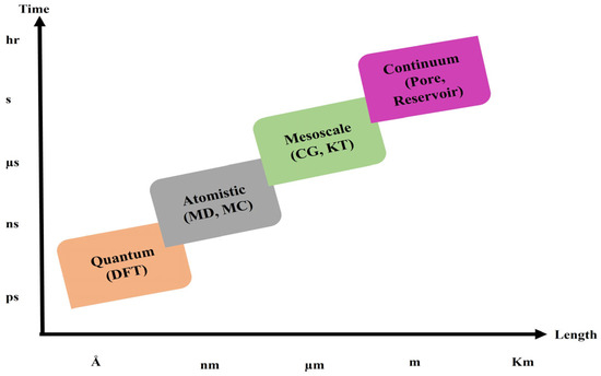
Figure 1. Current time and length scales for the main modeling approaches for subsurface phenomena [11].

Figure 2 demonstrates the diagram that depicts a step-by-step process for constructing a model for molecular simulation. The first step is to set up the initial conditions, which include specifying the number and type of molecules in the system, as well as their initial positions and velocities. The second step is to select a force field, which is a set of equations that describes the interactions between the molecules. The third step is to select the periodic boundary condition, which specifies how the simulation cell will be replicated to create an infinite system. The fourth step is to select the time step, which is the amount of time that will elapse between each step of the simulation. After the model has been constructed, the system can be equilibrated, which involves simulating for a long time to allow the system to reach equilibrium. Finally, data can be collected from the simulation, which can be used to calculate a variety of properties of the system [8,9,10].

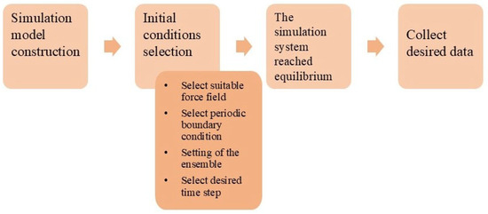
Figure 2. Molecular simulation step diagram [7].

The process of molecular dynamics simulation involves the following stages [7]:

• Simulation Box

The investigation of any phenomenon involves the utilization of two separate spaces: system or volume control, and environment, which are separated by a boundary according to the principle of thermodynamics. The simulation box is the boundary that separates the built system from its surroundings in the science of molecular dynamics and its simulations. The simulation and calculations are carried out on the target system inside the simulation box. This simulation box can be of different shapes, such as a cube, a rectangular cube, a trapezoid, a cylinder, etc. Different software supports different modes of this box. One of these models can be used for different simulations according to the purpose of the simulation [7,8,9,10].

• Force field (FF)

By utilizing numerical integration to solve the applicable Newton’s equation of motion for any atom in a molecular structure, the MD simulation approach calculates the atomic motion of molecules. Macroscopic features of the system are obtained by monitoring the trajectories and velocities of particles as a function of their interactions across time, and by utilizing statistics. The atoms and molecules assigned interaction potentials are determined by the appropriate FF model [12]. According to Figure 3, the FF model can be easily characterized as an arrangement of springs and rubber balls that represent atoms and their bonds, respectively [13]. The intramolecular and intermolecular interactions of this representation are highlighted by bonded and non-bonded energies. Bonded potential energies include interactions among the linked atoms via springs (bond forces), with hinges (valence angle potentials), and four-body interactions of proper and improper dihedral interactions. Coupled with the coulombic interaction and the Lennard–Jones (LJ) potential term, the interactions of intermolecular forces include coupled short-range repulsive Pauli exclusion forces and attractive van der Waals (vdW) forces [8,10,12].

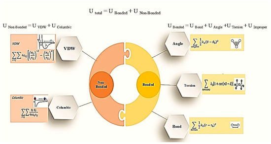
Figure 3. Force field formula [13].

Although MD provides a force field-based simulation, choosing an appropriate FF for the system is crucial. In general, numerous forms of force fields have been generated to simulate distinct molecules. The most popular of them are recognized as OPLS-AA (optimal parameterization for the liquid state) [14], CHARMM27 (chemistry at Harvard macromolecular mechanics) [15], CGenFF (CHARMM General Force Field) [16,17], COMPASS (condensed-phase optimized molecular potentials for atomistic simulation studies) [18], etc.

• Ensemble

An ensemble, which illustrates specific circumstances utilized in simulation systems, is another crucial concept in MD simulation. Every ensemble essentially isolates the simulation system from altering the particle numbers or both of the aforementioned variables: temperature, pressure, volume, and energy [19]. For MD simulation, ensembles often display the constancy of pressure and temperature (NPT), the dynamics of particle movement and interaction (NVT), and the preservation of total energy (NVE). The NVE ensemble maintains a constant number of molecules, their volume, and their internal energy due to the absence of heat transfer with the external surroundings. The MD trajectory is established when potential and kinetic energy are exchanged. Volume (V) and temperature (T) are the constant characteristics in the NVT ensemble. To maintain the temperature, a thermostat is employed. The common thermostats are Nose–Hoover [20], Berendsen [21], Anderson [22], and velocity scaling [23]. In addition to temperature, barostats like Parinello–Rahman [24] and Berendsen have been employed in the NPT ensemble to fix pressure.

• Cut off radius

The cutoff radius in a molecular dynamics (MD) simulation is a distance used to approximate how far interactions between atoms are important. It essentially creates a spherical boundary around each atom (Figure 4). Interactions between atoms within this radius are calculated explicitly, while those beyond are neglected [12]. Using a larger cutoff radius makes the simulation more accurate by accounting for more interactions, but it also increases the computational cost. A typical cutoff radius is around 2.5 times the sigma (σ) value, which represents the distance at which the repulsive and attractive forces between atoms cancel out in the Lennard–Jones potential. Another rule of thumb is to keep it less than half the size of the simulation box [7,8,9,10].

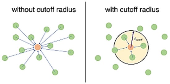
Figure 4. The concept of cutoff radius in molecular dynamics simulation is used in two ways: simulation with a cutoff radius and without a cutoff radius.

• Boundary condition

Boundary conditions in molecular dynamics (MD) simulations are a set of rules that define how particles behave at the edges of the simulation box. Since a real system is infinite, these conditions are crucial to mimic a larger system within a finite computational space. There are two common types of boundary conditions used in MD simulations [8,9,10,12]:

❖

Periodic Boundary Conditions (PBCs): This is the most widely used type. It essentially creates a repeating pattern of the simulation box. This creates the illusion of an infinitely repeating system and eliminates the unphysical effects introduced by a finite simulation box. PBCs are particularly useful for studying bulk properties of liquids, gases, and some solids. Figure 5 demonstrates the periodic boundary condition in three dimensions.

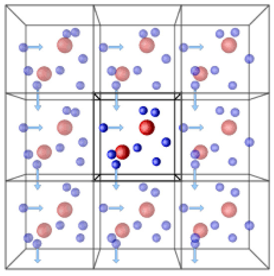Figure 5. Periodic boundary conditions (PBCs) in molecular dynamics simulations are used to create a repetitive and infinite set of molecules to increase accuracy.

❖

Fixed Boundaries: In this approach, the atoms at the edges of the simulation box are fixed in place. These fixed atoms can mimic the presence of a wall or a surface. However, fixed boundaries can introduce unphysical effects near the edges, as the real system would not have these abrupt stops. This method is sometimes used for studying thin films or interfaces, but with caution due to the potential artifacts.

1.1.2. MD Software

The simulation calculation method relies on computer software for support. With the development of computer science, a wide variety of simulation software has emerged, each with its own capabilities. Molecular simulation can be divided into three types: atomic, coarse-grained, and mesoscopic simulations. These types are based on the scale of the simulation. Different groups are assigned to the simulation software. The primary focus is on investigating electronic impacts, such as Gaussian and VASP, in this area of research. Utilized concepts include ab initio, fundamental principles, and the theory of density functional. The second classification primarily mimics the motion of molecules. GROMACS, AMBER, LAMMPS, and Material Studio are examples of software found in this category. The fundamental theoretical concept is the mechanics of molecules, focusing on the macroscopic properties of the system. Indeed, CHARMM, NAMD, and similar software are simulations that incorporate both approaches, too [7]. In Table 1, the merits and defects of the different types of the mentioned simulators are provided.

Table 1. Molecular dynamics simulators [7].

	Software	Range of Application	Research Content	Merit	Defect
1	Gaussian	Research on molecules	Mechanism of chemical reaction, impact of substituting elements, and simultaneous intermediate stages and transition structures	high level of accuracy in calculation	This only applies to minuscule systems because to calculation is laborious and time-consuming.
2	VASP	Research on Surface, Solid, and Atomic Structures	The theory of density functions provides a framework for solving the Kohn-Sham equation.	Swift computation performance and an effective algorithm for optimization	slow entrance
3	GROMACS	Investigation of molecular dynamics structures for numerous particle simulations	Solve the traditional Newton mechanical equation for a macromolecular structure.	Excellent functionality, quick computation times, and exceptional service for maintenance	Poor compatibility
4	AMBER	Investigation of conventional chemical molecular structures and systems of biology	-	highly built-in potential energy algorithms and simple molecular customization	Inadequate computational performance, snail-paced running, and costly purchase.
5	LAMMPS	molecular modeling investigation	Simulating particles in different states, including liquid, solid, and gas. Mimicking two or three-dimensional systems can be achieved with either a small or a large number of particles.	Sophisticated programming, excellent computational performance, and compatibility with the majority of potential energy models currently available	Lack of mapping output data, insufficient field parameters, inadequate maintenance, and unavailability of tools for creating molecular systems
6	Material Studio	Research for materials science	Predicting the characteristics of a material, creating structures of polymers, and modeling the scattering of X-rays.	Assists in working across a variety of devices, utilizes intelligent techniques, and is user-friendly.	Costly, not adept at distributing, and not very effective at multitasking.
7	CHARMM	Biological and chemical Structure investigation	-	The potential energy model has been quickly modified, allowing for easy customization and effective maintenance.	The software is slow and not efficient at processing math tasks, so a payment is required for its use.
8	NAMD	Biological and soft chemical substance investigation	-	Well-designed program, high compatibility and easy maintenance.	-

1.2. Molecular Structure of Oil and Injection Fluids

The presence of two immiscible fluids is necessary for the interfacial tension to exist. In molecular simulation, more intricate material structures require more mathematical computations, which increases the cost and runtime requirements. The required parameters must be verified by considering an appropriate component and making it simple. Neither a system too simple to accurately represent the proposed system nor too complex to require a lot of time and expense should be used for this component [7,8].

1.2.1. Different Types of Oil Structure

A mixture of hydrocarbons is found in natural gas and petroleum: 85% C, 13% H, and 2% each of N, S, and O (weight percentage) compose their average composition. Three categories represent the fundamental elements of natural hydrocarbons [25]:

• Paraffin: The usual formula for paraffin, often known as n-alkanes, is C_nH_2n+2. Gases correspond to n = 1 to 4, liquids to n = 5 to 15, and solids (paraffin waxes) to n ≥ 15.
• Naphthene, which has the general formula C_nH_2n, produces saturated ring compounds when n is one of the following: 5, 6, or 7. A typical crude oil will contain 2% or more of the common components cyclopentane and cyclohexane, which are frequently observed in the methylated state.
• Aromatics: aromatics are hydrocarbons that are commonly classified as a minor category since they share a fourth bond with all carbons in at least one benzene ring (C₆H₆). Due to their ability to react and add hydrogen or other elements to their rings, they are known as undersaturated.

The structure of oil can be considered in different ways. Oil can be classified as olefinic (mixture of naphthene and paraffins), aromatic (including benzene, toluene, and cyclic compounds like asphaltene, resin, and cycloalkanes), or a combination of the two. It is possible to include asphaltene in the simulation oil or to model it without asphaltene [25].

Although the heavier components of crude oil have been investigated, researchers are still unfamiliar with asphaltenes, a particular type of organic material. Asphaltene has been investigated by chemists, chemical engineers, petroleum engineers, and material engineers for decades. Their studies aim to identify the basic components of asphaltenes to comprehend their behavior within crude oil. This will assist us in forecasting asphaltene characteristics like deposition and surface activity. Various laboratory techniques and characterization tests were employed to determine the molecular weight, aggregation mechanism, aggregate structure, size, architecture, and shape [26].

Asphaltene is composed of a variety of molecules, resulting in a complex structure composed of heteroatoms, heterocycles, polyaromatic groups, alkyl-chain functional groups, and sulfur, nitrogen, and oxygen atoms. Consequently, the molecular level experiences differences in its characteristics and mechanisms. The use of molecular dynamics simulation has greatly improved our understanding of asphaltene and its self-association, deposition, and aggregation. In atomistic simulations, it is frequently accepted that a single asphaltene molecule can be used to represent a larger set of similar molecules. Due to the diverse range of sizes, it is doubtful that only one type of molecule can be effectively characterized as asphaltenes. Due to practical considerations, most studies are bound to have limitations. The limited computational capabilities of our computers mean that only a small number of molecules are typically examined, making it hard to accurately characterize asphaltenes through experimentation [27].

Islands and archipelagos are the two main types of asphaltene structures. The general structure of island shapes consists of a central aromatic or heteroaromatic core, along with several alkyl chains extending from it. Archipelago forms typically consist of multiple interconnected aromatic and heteroaromatic rings linked by alkyl bridges [28]. An example of the island and archipelago types of asphaltene structure molecules is given in Figure 6.

Figure 6. Representation of different types of asphaltene molecule: (a) Island-type (C₅₁H₆₂S) [29] (b) Archipelago-type (C₉₇H₁₁₇NO₄S₄) [30].

1.2.2. Injection Fluid Structures

The EOR usually corresponds to the injection of gases, water, and chemical substances like polymers, surfactants, etc. To simulate numerous scenarios occurring throughout the EOR process, it is necessary to know the molecular structure of each component in the system.

The dissolved salt and the type of water molecule played an important role in the accuracy and reliability of brine injection simulation results. Water is probably the most versatile medium, as it is present in most EOR processes and various mixtures and material dissolutions. Thus, it can serve as the basis for all molecular dynamics simulations in biological phenomena, as well as a fair number of interdisciplinary chemical, industrial, and materials investigations. Over the years, several water models were developed, and finding a single water model that accurately and completely simulates all experimental characteristics of water still poses a challenge. There are four types of water molecule models: (a) three-point, (b) four-point, (c) five-point, and (d) polarizable, which are reported in Figure 7.

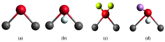
Figure 7. Geometry of water molecule models; oxygen is red and hydrogen is grey, the offset partial charge on oxygen, M, in four-point is pale blue. The long pairs, L, in the five-point are light green, and the Drude oscillator in polarizable is purple.

Pathirannahalage et al. [31] recorded a comprehensive comparison of structural and dynamic properties of 30 commonly used 3-point, 4-point, 5-point, and polarizable water models simulated based on FF parameters like bond lengths, partial charges, LJ coefficients, etc., consistently regarding settings and methods of analysis; some of the results are provided in Table 2.

Table 2. Water molecule models characterization [31].

No.	Name	Type	Flexibility	Density (g/cm3)	IFT (mN/m)	Published Year
1	SPC	3-point	No	0.972 ± 0.006	50.3 ± 0.2	1981
2	TIP3P	3-point	No	0.980 ± 0.006	47.0 ± 0.2	1983
3	TIP4P	4-point	No	0.994 ± 0.006	52.2 ± 0.2	1983
4	TIPS3P	3-point	No	1.007 ± 0.006	51.1 ± 0.2	1985
5	SPC/E	3-point	No	0.993 ± 0.006	57.6 ± 0.2	1987
6	CVFF	3-point	Yes	0.978 ± 0.006	47.3 ± 0.4	1988
7	TIP3P/Fw	3-point	Yes	1.027 ± 0.006	55.2 ± 0.4	1999
8	TIP5P	5-point	No	0.985 ± 0.006	47.1 ± 0.2	2000
9	TIP3P-Ew	3-point	No	0.996 ± 0.006	59.2 ± 0.2	2004
10	TIP4P-Ew	4-point	No	0.996 ± 0.005	52.2 ± 0.2	2004
11	TIP5P-Ew	5-point	No	1.003 ± 0.006	63.5 ± 0.2	2004
12	TIP4P/2005	4-point	No	0.997 ± 0.005	63.5 ± 0.2	2005
13	TIP4P/Ice	4-point	No	0.993 ± 0.006	73.4 ± 0.2	2005
14	SPC/Fw	3-point	Yes	1.007 ± 0.006	58.6 ± 0.4	2006
15	SWM4-NDP	Polarizable	No	0.990 ± 0.005	63.1 ± 0.5	2006
16	TIP4P/2005f	4-point	Yes	0.996 ± 0.005	60.3 ± 0.4	2011
17	TIP4P/ε	4-point	No	0.996 ± 0.006	64.6 ± 0.2	2014
18	OPC	4-point	No	0.997 ± 0.005	70.1 ± 0.2	2014
19	TIP3P-FB	3-point	No	0.990 ± 0.006	60.3 ± 0.2	2014
20	TIP4P-FB	4-point	No	0.997 ± 0.006	64.7 ± 0.2	2014
21	TIP4P-D	4-point	No	0.993 ± 0.006	70.8 ± 0.2	2015
22	SPC/ε	3-point	No	0.991 ± 0.005	65.3 ± 0.2	2015
23	OPC3	3-point	No	0.991 ± 0.006	61.0 ± 0.2	2016
24	a99SB-disp	4-point	No	0.996 ± 0.006	74.4 ± 0.2	2018
25	TIP5P-2018	5-point	No	0.997 ± 0.006	61.6 ± 0.2	2018
26	TIP3P-ST	3-point	No	0.993 ± 0.005	63.8 ± 0.2	2019
27	TIP4P-ST	4-point	No	0.999 ± 0.006	64.5 ± 0.2	2019
28	FBA/ε	3-point	Yes	0.991 ± 0.005	68.0 ± 0.4	2020

1.3. Experimental Methodology of IFT Measurement

Experimentally, IFT can be measured by several techniques, such as Wilhelmy plates, the Du Nouy ring, maximum bubble pressure, capillary rise, drop volume, pendant drop, and sessile drop. Here, these methods are summarized.

1.3.1. Force Tensiometry Methods

The process of measuring interfacial tensions directly with a microbalance involves bringing a plate, ring, rod, or other simple-shaped probe into contact with the interface. If one of the liquids completely wets the probe, the liquid will adhere to it and rise due to capillary force, expanding the interfacial area and producing a force that tends to pull the probe toward the interface plane [32]. This restoring force is instantly associated with the interfacial tension and can be calculated with a microbalance. The force (F) operating across the three-phase contact line is particularly equivalent to the weight of the liquid meniscus positioned above the fluid–fluid interface plane. This force, calculated with a microbalance, is utilized to compute the interfacial tension:

$$\gamma = {\displaystyle \frac{F}{P Cos \theta }}$$

(2)

• Wilhelmy Plate Method: This method involves measuring the force required to pull a thin plate partially submerged in the liquid interface upwards, as demonstrated in Figure 8. The interfacial tension is calculated based on the measured force, plate dimensions, and contact angle. By measuring the mentioned force, the interfacial tension can be calculated using Equation (2), where p = 2 (L + t) [33].
  

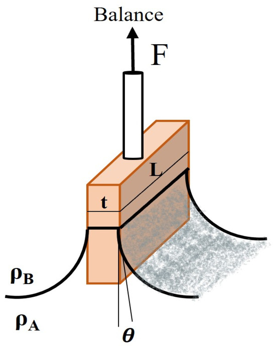  Figure 8. Illustration of Wilhelmy plate method [33].
• Du Nouy Ring Method: This method involves measuring the force required to pull a wire ring partially submerged in the liquid interface upwards (Figure 9). The interfacial tension is related to this force through the ring’s geometry and the contact angle between the liquid and the ring. The ring circumference is equivalent to twice the perimeter (p) of the three-phase contact line in this case: p = 4$\mathsf{\pi }$ R. Equation (2) requires a correction factor (f) because more liquid is lifted during the ring’s separation from the interface [34]:
  

  Figure 9. A schematic of the Du Nouy Ring Method [34].

$$\gamma ={\displaystyle \frac{F}{P Cos \theta }} f$$

(3)

$$\mathrm{F}=0.725+(\frac{9:075.{10}^{-4}\mathrm{F}}{{\mathsf{\pi }}^3{∆\mathsf{\rho }\mathrm{R}}^3}-\frac{1.679 r }{R}0:04534{)}^{1/2}$$

(4)

The application range of Equation (4) is 0.045 < ${\mathsf{\pi }}^3{∆\mathsf{\rho }\mathrm{R}}^3$ < 7.5.

1.3.2. New Techniques (Based on Capillary Pressure)

Positive interactions between immiscible phases tend to reduce interfacial tension, or the work needed to produce an interface unit area. The Young–Laplace equation explains this as pressure differences that cause capillary rise, bubble, and drop formation [35]:

$$∆P= \gamma ({\displaystyle \frac{1}{R1}}- {\displaystyle \frac{1}{R2}})$$

(5)

• Maximum Bubble Pressure Method: This method involves forcing a gas bubble to grow at the tip of a submerged tube. As the pressure inside the bubble increases, it counteracts the interfacial tension at the bubble’s surface (Figure 10). The pressure at which the bubble detaches from the tube is related to the interfacial tension. This method is particularly useful for studying high interfacial tension systems [36].
  

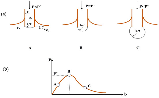  Figure 10. Maximum bubble pressure method. (a) A sequence illustrating the shape of a bubble at three different stages of bubble growth. (b) Relationship between pressure inside the bubble and radius of the bubble, b is the curvature radius [36].

Calculation of the interfacial tension can be done by using the following equation:

$$\gamma = {\displaystyle \frac{∆P r }{2}} (1- {\displaystyle \frac{2r ∆\rho g }{3 ∆P}}- {\displaystyle \frac{{\left( r ∆\rho g \right)}^2}{6 ∆P^2}})$$

(6)

• Capillary Rise Method: This method utilizes the phenomenon where a liquid rises inside a narrow tube inserted vertically into the liquid, as shown in Figure 11. The height (h) to which the liquid rises depends on the interfacial tension ($\gamma )$, the tube diameter (r or d), and the liquid’s density ($\rho )$. It is a relatively simple method, but it requires careful control of factors like tube cleanliness [37].
  

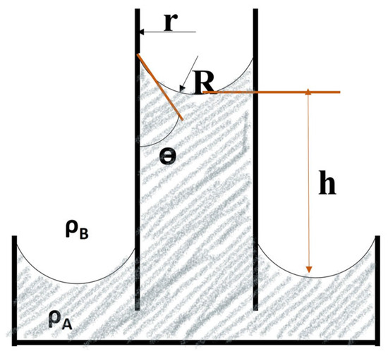  Figure 11. A schematic of the capillary rise method [37].

The following formula can be utilized for calculating surface tension since the meniscus has a spherical shape:

$$\gamma = {\displaystyle \frac{∆\rho ghr}{2 cos\theta }}$$

(7)

• Spinning drop method: The method of spinning drops involves evaluating the surface tension of a liquid by examining the characteristics and size of a droplet that appears on the surface of a different liquid during spinning under the mechanical equilibrium of interfacial force and centrifugal force (Figure 12) [38].
  

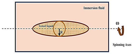  Figure 12. A schematic of the spinning drop method [38].

IFT could be determined by this method with Vonnegut’s expression equation [38]:

$$\gamma = {\displaystyle \frac{∆\rho {\omega }^2}{4}} R^3$$

(8)

where ω is the angular velocity and $∆\rho$ is the density difference between the droplet and immersion fluid.

1.3.3. Optical Tensiometry Methods

• Drop Volume Method: This method involves determining the minimum volume of a drop required to detach from a tip (like a needle) due to its own weight. The interfacial tension is related to the drop volume and the tip geometry. This method is relatively simple but can be less accurate than other techniques. Figure 13 demonstrates the drop volume method for calculating IFT [39].

Figure 13. Illustration of the drop volume method [40].

• Pendant Drop Method: This method is also known as axisymmetric drop shape analysis (ADSA). It involves analyzing the profile of a liquid drop suspended at the tip of a needle or pipette within another liquid, as shown in Figure 14. The software fits the drop shape into a theoretical model that incorporates interfacial tension. This method is advantageous because it allows for non-intrusive, continuous monitoring of interfacial tension [41,42,43].
  

  Figure 14. A schematic of a pendant drop.

The interfacial tension is then calculated from the following equation:

$$\gamma = {\displaystyle \frac{∆\rho gg D^2}{H}}$$

(9)

where the shape-dependent parameter (H) depends on a value of the “shape factor of S = d/D” [43].

• Sessile Drop Method: This method is similar to the pendant drop method, but instead of hanging from a tip, the liquid drop sits on a solid surface (Figure 15). The software analyzes the drop’s contact angle with the solid surface and its overall profile to determine the interfacial tension. This method is useful for studying solid–liquid interfaces [35].
  

  Figure 15. A description of the sessile drop’s dimensions and coordinates.

To determine the height via the top of the drop to its equator (z_e), one must first identify the drop’s equator using a straightforward experimental method. An analytic formula for the interfacial tension for an extremely big sessile drop is as follows:

$$\gamma = {\displaystyle \frac{∆\rho g z{e}^2}{2}}$$

(10)

Choosing the most appropriate method depends on the specific system being studied, the desired level of accuracy, and the available equipment. Some methods are simpler to set up but might be less accurate, while others require specialized equipment but offer better precision. In Table 3, the accuracy and application of the mentioned methods are summarized.

Table 3. The appropriateness and accuracy of the aforementioned methods for measuring IFT [35].

Method	Accuracy (mN/m)	Surfactant Solutions Compatibility	2-Liquid Phases Compatibility	Viscous Liquids Compatibility	Commercial Accessibility
Wilhelmy plate	~0.1	Restricted	Adequate	Great	Available
Du Nouy ring	~0.1	Restricted	Reduced accuracy	Inappropriate	Available
Maximum bubble pressure	0.1–0.3	Great	Great	Inappropriate	Available
Capillary rise	Less than 0.1	Great	Great (experimentally difficult)	Inappropriate	Available
Drop volume	0.1–0.2	Restricted	Adequate	Inappropriate	Available
Pendant drop	~0.1	Great	Great	Inappropriate	Available
Sessile drop	~0.1	Adequate	Great	Great	Available

1.3.4. Molecular Dynamics Simulation of IFT

The Kirkwood and Buff approach, or the integral given in Equation (11), was used to compute the IFT (${\gamma }^{KB}$) of the two phases with interfaces n = 2 [44,45,46]. The simulation was run with the three diagonal components of the pressure tensor (i.e., $P_n=P_{zz}$ and P_t = $({\displaystyle \frac{P_{yy}+P_{xx}}{2}})$) calculated, and the output interfacial tension values were averaged in time blocks. Ultimately, the run time was averaged to determine the equilibrium IFT.

$${\gamma }^{KB}={\int }_0^{Lz}\left(P_{n\left(Z\right)}-P_{t\left(Z\right)}\right)dz={\displaystyle \frac{L_Z}{N}}(P_{zz}-{\displaystyle \frac{P_{xx}+P_{yy}}{2}})$$

(11)

where P_n is the normal component of the pressure tensor, P_t is the tangential component of the pressure tensor, and L_z is the length in the z-direction of the simulated system [46].

The selection of specific oils and injection fluids (carbon dioxide, saline water, etc.) necessitates adopting the required type of simulation system in time to study the behavior of molecules in oil and injection fluids. The most stable states of the molecular structures of oil and injection fluids are designed with Avogadro and Material Studio. Packmol is then used to develop a simulation box in which the molecules are placed before the relevant force field files and input scripts for the simulator are created. The simulation is run via the Linux terminal as per these files for the desired run-time.

The requested outputs are to be found in the output files. Within this study, the prime focus is on the interfacial tension (IFT). To measure this, the simulator keeps track of the simulation box size and the pressure tensor components at every time step to calculate the respective IFT values using the established formula. By plotting time versus IFT, we can observe the behavior of IFT in equilibrium.

For instance, Li et al. [46] employed molecular dynamics to determine the interfacial tension of CO₂–brine systems in higher temperature (303–393 K) and pressure (2–50 MPa) conditions. This showed that under all temperature conditions, IFT decreases with increasing pressure but increases linearly with brine salinity. Similarly, de Lara et al. [47] conducted MD simulations on interfacial effects in brine (H₂O + NaCl), CO₂, N₂, CH₄, and crude oil in the context of improved oil recovery (IOR) processes. In most cases, the results showed aromatic molecules being accumulated near the interface, and further that the trends of IFT depend strongly on the type of fluid: brine/crude oil generally has a positive correlation with increasing pressure and salinity, while increasing pressure and temperature largely cause the reduction in IFT for CO₂, N₂, and CH₄.

2. Effective Parameters on IFT

The interfacial tension between two phases (e.g., liquid–liquid or liquid–vapor) is influenced by various parameters. These parameters can have complex interrelationships and may influence the interfacial tension through various mechanisms. Here are some of the key parameters that can affect interfacial tension [48,49,50]:

• Temperature: Interfacial tension generally decreases with increasing temperature due to increased molecular motion and decreased intermolecular forces.
• Pressure: Interfacial tension between liquid and vapor phases is affected by pressure.
• Oil and injection fluids composition.
• Solvent properties:

  ❖

  Polarity and dielectric constant of the solvents.

  ❖

  Dispersion forces and hydrogen-bonding capabilities.

  ❖

  Miscibility and mutual solubility.

• Electrolyte concentration: The presence of ions can alter the interfacial tension due to electrostatic interactions and screening effects.
• External fields (e.g., electric or magnetic): Applied external fields can induce changes in the interfacial tension, particularly for systems involving charged or polarizable species.

In this section, a summary of previous studies focused on measuring interfacial tension through experimental methods and molecular dynamics simulations is provided. In Table 4, Table 5 and Table 6, the results of lab experiments and molecular dynamics simulations focusing on the effect of gas and water injection, temperature, pressure, and the oil composition are summarized.

Table 4. Interfacial tension of Oil–CO₂.

No.	Oil Comp	Gas System	T (K)	P (MPa)	Method	Results	Ref
1	Heptol (0.0:1.0, 0.25:75, 0.5:0.5, 0.75:0.25, 1.0:0.0)	CO2	344.15	0.1–8	Experimental + (SGT + SAFT VR Mie EOS model)	At a constant temperature, an increase in pressure causes an IFT reduction	[51]
2	2 oil types (20.2 & 20.75 API)	CO2	313.15, 333.15, 353.5, and 373.15	0.68, 3.44, 6.89, 8.96, 11.72, 15.16	Experimental	1. As the temperature increases in the low-pressure area, the IFT decreases. 2. There was a change in trend at 6.89 MPa, and as the temperature increased, the IFT started to increase. The reason for this is that when the temperature goes up, CO2 dissolves more easily in crude oil. This makes the tension between the oil and water less when the pressure gets low. 3. At a constant temperature, IFT reduces due to pressure increase with two different trends, and these two different line connection points provide asphaltene offset	[52]
3	3 types: heptane, hexadecane, Diesel fuel	CO2	313.15, 333.15, 353.5, 373.15, and 393.15	0–16	Experimental	1 Less pressure (up to 5. Increasing the temperature is found to be most effective for extracting CO2 oil at a low pressure (up to 5.17 MPa), as it reduces all interfacial tensions. 2. Regardless of the temperature, the IFT remains constant at 5. 17 MPa, forming a stable connection. Injecting carbon dioxide at this pressure is not advisable. 3. As the pressure increased, it was more effective to inject CO2 into reservoirs with lower temperatures due to the positive correlation between interfacial tension vs. temperature.	[53]
4	Alkanes & aromatic elements	CO2, N2, CH4	300, 350	0.1–30.397	MD (LAMMPS)	1. More favorable oil displacement when pressure and salt concentration increase because of IFT increase & aromatic molecules accumulate near the interface has been investigated. 2. Due to the increase in pressure and temperature, IFT for gases reduces, and gas diffusion in the oil increases.	[47]
5	n-decane	CO2	344	1–13	MD (LAMMPS)	Interfacial tension decreases with increasing pressure	[54]
6	n-alkane	CO2	323.15, 353.15	Up to 17.4	Exp (Pendant drop)	1. IFT decreases with an increase in pressure and temperature at lower pressures. 2. These trends reversed for higher pressure, which leads to an increase in MMP with temperature increase. 3. Heavier oil (long-chain n-alkane) leads to MMP. increase	[55]
7	decane-iododecane (mass fraction of 0%, 50%, 70%, 90% and 100%)	CO2	298, 313, 333, 353	1 up to the TC of the mixture	Exp (Pendant drop)	1. Due to pressure and mass fraction of iododecane increasing the IFT decreases. 2. An increase in mass fraction in iododecane causes an increase in Tc of the mixture. 3. An overall average absolute deviation of 0.2 mN∙m−1 was reported between experimental data and the developed empirical model.	[56]
8	Model oil (45wt% of C16H34, 45wt% of C20 H42, 10wt% of C24H50)	CO2, CO2 +brine	333.15	Up to 25	Exp (pendant drop)	1. IFT decreases due to the pressure increase in both binary and ternary mixtures 2. In a ternary system, as pressure increases, the IFT decreases due to CO2 acting amphiphilic molecule between coexisting immiscible phases. 3. In the ternary mixture, the IFT reaches its maximum value at high salt concentrations.	[57]
9	n-decane, n-hexadecane, (n-decane + n-hexadecane)	CO2	313.15, 333.15	0.1–16	Exp (pendant drop)	1. Pressure increasing, temperature reduction, and larger chain length of hydrocarbon cause IFT reduction. 2. A light compound in flooding gas has a significant cosolvent effect, enhancing miscibility between large alkanes and CO2, as indicated by lower IFT and MMP values.	[58]
10	Organic liquid (Cyclohexane, ethanol, Octane, hexane)	CO2	308.15, 323.15, 333.15	3.6, 5.6, 6, 7.6	Exp (pendant drop)	1. As pressure increases and temperature reduces, CO2-organic liquid reduces. 2. Important factors influencing the IFT of CO2 and organic liquids are the intermolecular force that exists among their molecules and the organic liquid’s polarity and structure.	[59]

Table 5. Interfacial tension of CO₂–Brine.

No.	Brine Com	Gas	T (K)	P (MPa)	Method	Results	Ref
1	NaCl, CaCl2	CO2	303–393	2–50	MD with GROMACS	1. At every temperature, due to an increase in pressure, IFT decreases. 2. With salinity increases, IFT has a linear increasing trend.	[46]
2	pure water	CO2	275.15, 298.15	up to 4	MD with DL_POLY	Upon pressure increase, the IFT reduces due to the adsorption of more molecules at the interface.	[60]
3	Water	CO2	278.15–344.15	0.1–17	Experimental (capillary rise method)	IFT decreases as pressure increases.	[61]
4	Water	CO2	278–333	0–25	Experimental (Pendant drop method)	1. Pressure has a greater impact on reducing IFT when the temperature is low. 2. IFT decreases with an increase in temperature at low pressures; vice versa, increasing the temperature under high pressure results in an increase in IFT.	[62]
5	Brine	CO2	300.15, 331.15	0–30 MPa	Experimental (Pendant drop method)	IFT increases as pressure reduction & temperature increase	[63]
6	Water	CO2	318.15	0–17	Experimental (Pendant drop method)	As the pressure rises, the IFT reduces significantly before reaching a plateau at high pressure.	[64]
7	H2O + 20 g/L NaCl	CO2	308–383	5–45	Experimental (Pendant drop method)	The IFT experiences a substantial decrease with increasing pressure, followed by a plateau and a slight decline as the temperature rises. Adding 20 g of salt to water doesn’t have a significant impact.	[65]
8	0–334 010 mg·L−1	CO2	293–398	2–27	Experimental (Pendant drop method)	1. At P < Pc, with pressure increase, the IFT reduces. 2. At temperature & pressure, as increase in salinity the IFT increases too. 3. At temperatures that are equal to or greater than Tc, due to temperature increases, the IFT increases too.	[66]
	Water	CO2–H2S mixture (with 30 mol% H2S)	313, 343,393	0–15	Experimental (Pendant drop method)	Due to increasing H2S content, the IFT reduced sharply.	[67]
9	(0–334,000 mg/L) formation brine	CO2	309–398	2–27	Experimental (Pendant drop method)	Pressure increase and temperature decrease cause IFT reduction.	[68]
10	(0–334,000 mg/L) formation brine	CO2	293–398	2–27	Experimental (Pendant drop method)	1. A decrease in pressure results in a decrease in IFT, which then plateaus at higher pressure levels. 2. Salinity increases cause an increase in IFT. 3. At T < Tc, an increase in temperature causes the IFT to increase. At T = Tc, temperature increases cause noticeably reduced IFT. At T > Tc, the IFT stabilizes at a constant value asymptotically.	[66]
11	0–2.75 mol/L NaCl	CO2	300.15, 344.15, 373.15	5–25	Experimental (Pendant drop method)	Pressure causes the IFT to decrease and maintain a consistent level independent of salinity. The pressure needed to reach this plateau increases with the rising temperature. As the temperature increases, so does the IFT. IFT rises alongside the concentration of NaCl.	[69]
12	0.045–2.7 mol/L CaCl2	CO2	300.15, 344.15, 373.15	5–25	Experimental (rising drop method)	As pressure increases, the IFT decreases, but then stabilizes once the pressure stops rising, regardless of the liquid’s saltiness. There is not much information available about how temperature influences IFT. An increase in salinity causes the IFT to rise.	[70]
13	Saltwater is produced by dissolving natural halite crystals in water.	CO2	296.5 ± 1.5	0.1–20	Experimental (Sessile drop method)	As the pressure rises, the IFT experiences a sharp drop followed by a plateau.	[71]
14	Water	CO2	298–374	1–60	Experimental (Pendant drop method)	IFT decreases as pressure rises. The change in IFT for isotherms at temperatures 297.9, 312.9, and 333.5 Kelvin can be split into two parts. The slope of the decrease in IFT at temperatures 343.3 and 374.3 shows a more gradual change.	[72]
15	NaCl (0.045–1.5 mol/L) & (0.045–1.5 mol/L) CaCl2	CO2	300.15, 344.15, 373.15	5–25	Experimental (rising drop method)	1. There is a downward trend in the IFT, with the rate of decrease also diminishing for each temperature point. The IFT reaches a constant value as the pressure increases and the temperature changes. 2. From 300.15 < T < 344.15 & pressures P < P plateau, IFT increases 3. From 300.15 < T < 373.15, the IFT remains relatively constant. 4. An increase in salinity causes the IFT to rise.	[70]
16	Water	CO2	298.15–333.15	1.48–20.76	Experimental (Pendant drop method)	1. At low pressure, where CO2 CO2-rich phase is gaseous, an increase in pressure causes the IFT reduction. 2. At high pressure range where rich phase CO2 is liquid, IFT remains virtually unchanged.	[73]
17	NaCl + KCl (0.98–4.95 mol/kg)	CO2	298–448	2–50	Experimental (Pendant drop method)	1. Salinity effect: An increase in salt molality causes IFT to rise linearly. 2. Pressure effect: For P < Pc, an increase in pressure causes rapid IFT reduction afterwards, and IFT reduces gradually. 3. Temperature effect: There is a complex interrelationship between IFT & temperature.	[74]
18	CaCl2, MgCl2, Na2SO4 mixture (0.49–5.0 mol/kg)	CO2	343–423	2–50	Experimental (Pendant drop method)	1. An increase in salt molality causes IFT to rise linearly. 2. For P < Pc, an increase in pressure causes rapid IFT reduction afterwards, and IFT reduces gradually. 3. There is a higher IFT for divalent cations than monovalent cations.	[75]
19	brine (14,224.2 and 21,460.6 mg/L)	CO2	318.15, 370.68	0.1–36	Experimental (Pendant drop method)	At higher pressures, the IFT reaches a plateau after a rapid reduction as the pressure rises.	[76]
20	Deionized water	CO2	283, 298, 313	3, 4, and 5	Experimental (Pendant drop method)	The decrease in IFT is due to the increase in pressure and temperature reduction.	[77]
21	Brine	CO2	303–393	2–50	MD	At any temperature, as pressure rises & salt molality reduces, IFT reduces.	[78]
22	Brine (0.2–5 m/L)	CO2+ SO2 (0–6 wt%)	323.15–373.15	13.789–27.579	Experimental (Captive bubble method)	IFT doesn’t change due to pressure variation, as temperature increases have a minimal reduction and a linear reduction trend as the concentration of SO2 increases.	[79]
	Brine	CO2, N2 & CO2–N2 mix	333	13	Experimental (Pendant drop method)	IFTN2-brine > IFTCO2-brine ~ IFT N2/CO2-brine	[80]
23	NaCl (0.102, 1 mol/L)	CO2	300.15, 308.15 & 313.15	3–9	Experimental (Pendant drop method)	At high pressures and isotherms, IFT reduces and reaches a pseudo-plateau. At low pressure, the IFT increases as the temperature rises more quickly.	[81]
24	Water	CO2	296, 323 & 343	0.1–20	Experimental (Pendant drop method)	For P < 10 MPa, as the pressure increases, IFT reduces sharply afterwards, with a slight reduction trend observed. An increase in temperature causes the IFT to rise.	[82]
25	NaCl (0–30 wt%)	CO2	308, 323 & 343	0.1–20	Experimental (Pendant drop method)	An increase in temperature and salinity, pressure reduction, and the IFT increase.	[83]
26	NaCl (0–200,000 ppm)	CO2–CH4 mix	350.15–530.15	0.1–34.66	Experimental (Pendant drop method)	1. CO2 presence: CH4-brine IFT reduction. 2. Pressure effect:—at low pressure, IFT linear reduction. -at high pressure: slightly reduced. 3. Salinity & temperature: IFT increases as these two factors increase.	[84]
27	brine (NaCl, CaCl2 & NaCl + CaCl2)	CO2	343	20	MD	IFT alteration depends on cation valence. There is a linear correlation between IFT and ionic strength.	[85]
28	Water	N2,CO2 + N2	298.15–448.15	2–40	Experimental (Pendant drop method)	As increasing pressure & temperature cause the CO2 + N2/H2O and N2/H2O IFTs to reduce	[86]
29	NaCl (0–30 wt%)	CO2	323	15	Experimental (Pendant drop method)	A linear trend between IFT and salinity was observed.	[87]
30	CaCl2 & MgCl2	CO2	323	0–20	Experimental (Pendant drop method)	The decreasing pressure causes the IFT to lower gradually. The CO2/brine IFT increases sequentially with Mg2+ > Ca2+ > Na+ at a constant pressure, temperature, and salinity.	[83]
31	NaCl (0–1.8 mol/kg)	CO2	300–353	3–12	Experimental (Pendant drop method)	1. Salinity & temperature effect: An increase in these two factors causes IFT to rise. 2. Pressure effect: For P < Pc, an increase in pressure causes linear IFT reduction, and afterwards, IFT reduces gradually until it stabilizes.	[88]
32	NaCl (0.98, 1.98 mol/kg)	CO2	298–423	~69.51	Experimental (Pendant drop method)	As pressure increases, the IFT decreases, but the rate of decrease gradually slows until it stabilizes. Salinities have a positive impact on interfacial tension.	[89]
	NaCl (up to 14 wt%)	CO2	311–473	Up to 100	MD	An increase in temperature & pressure and a decrease in salinity cause an IFT reduction.	[90]
33	Distilled water	CO2	296–343	0.1–20	Experimental (Pendant drop method)	As the pressure increases, the interfacial tension also increases and then stabilizes. IFT decreases with temperature drops in low-pressure conditions. IFT increases with high pressure.	[91]
34	Brine (NaCl-CaCl2-KCl- MgCl2)	CO2	285–300	Up to 9	Experimental (Pendant drop method)	As the pressure increases, the interfacial tension also increases and then stabilizes. IFT decreases with temperature drops in low-pressure conditions. IFT increases with high pressure. IFT rises with both salinity & cation valence.	[92]
35	NaCl + KCl	CO2	298–373	3–15	Experimental (Pendant drop method)	IFT rises with both salinity & temperature and reduces with pressure until it reaches a plateau.	[92]
36	NaCl + CaCl2 + MgCl2 + KCl	CO2	308, 333	4.48–20	Experimental (Pendant drop method)	IFT reduces with pressure & rises with temperature.	[93]
37	NaCl (0–7 wt%)	CO2	353.15–453.15	8–22	Experimental (Pendant drop method)	IFT reduces with pressure & rises with temperature and salinity.	[94]

Table 6. Interfacial tension of Oil–Brine.

No.	Oil Comp	Brine omp	T (K)	P (MPa)	Method	Results	Ref
1	Heptol (50:50)	5, 15 wt% NaCl, CaCl2, Na2SO4	296.15	0.1	MDS (LAMMPS)	Even though non-polar hydrocarbons lack a functional group for ion accumulation, ions gather at the interface between charge-neutral hydrocarbons and brine. This leads to fluid layers that are alternately positively and negatively charged, giving the appearance of an electrical double layer. The composition of contacting electrolytes controls the charged layer strength near non-polar hydrocarbons, with the interfacial charge density following the toluene > heptol > heptane trend.	[95]
2	Medium oil, light oil, heptane, toluene, heptol	Sulfate and chloride	300	0.1	MDS(LAMMPS) + Machine Learning (ML)	The ML with 2% to 9% error from experimental data has better results	[96]
3	Heptol (0–100:0–100) + (0–0.01) wt% asphaltene	DI water with 0.93 g of NaCl & 0.67 g of NaHCO3	298.15–358.15	0.1	Experimental	1. An increase in the concentration of asphaltenes decreases the IFT. 2. The IFT decreased at first but later increased due to the precipitation of asphaltenes. 3. As the temperature increases, IFTs decrease.	[97]
4	2 oil types A,B	Reservoir brine	298, 333, 374, 383	17.237, 20.684, 24.132, 27.579, 31.026	Experimental & ML(LS-SVM)	1. An increase in the temperature, pressure, and salinity of synthetic formation water results in a higher IFT for reservoir A. 2. The IFT of oil reservoir B increases with an increase in pressure and salinity but decreases with a temperature increase. 3. The model provides an authentic prediction of the experimental IFT data.	[98]
5	Dodecane &octane+ toluene & benzene	0.0, 0.2,1, 2M NaCl	295.15, 323.15	0.1	MD with LAMMPS	1. The IFT increases with salinity. 2. Temperatures rising cause IFT reductions.	[45]
6	Heptol (0:100, 100:00, 56:44, 20:80 volume ratio) +VO-79 asphaltene (50 ppm)	Pure water	300	0.1	MD with GROMACS	An increase in modeled asphaltene concentration causes an IFT reduction	[44]
7	Dodecane, toluene, resins (quinoline & 3-naphthenic acid)	Pure water	300,600	0.1	MD with LAMMPS	There is a correlation between the gathering of oil at the interface and the tension existing between oil layers.	[99]

3. Discussions

Molecular dynamics simulation utilizing classical equations of motion became possible more than fifty years ago. Since then, the utilization of classical-physical molecular modeling in chemical research has developed significantly. It is extensively used in many different areas of chemistry and has made a substantial contribution to the advancement of chemical knowledge. It provides semiquantitative predictions for both measurable and non-measurable qualities of substances, assists in assessing and comprehending experimental results, and enables calculations of molecular system attributes in situations that are not accessible through experimentation [100].

However, the assumptions, approximations, and simplifications upon which molecular simulation is based reduce its accuracy and its range of applications. These relate to the methods used to compute specific attributes of chemical systems from statistical-mechanical ensembles, the potential-energy function that is employed, and the appropriate sampling of the large statistical-mechanical configurational space of a molecular system [100,101].

This review refers to literature on interfacial tension (IFT) measurements in CO₂-brine/oil systems and includes very critical factors governing the effectiveness of CO₂-EOR. Interfacial tension (IFT) is one of the parameters that indicates the impact of enhanced oil recovery (EOR) in oil reservoirs, so its determination is crucial. The review also indicated that several parameters, namely temperature, pressure, salinity, and the presence of asphaltenes, significantly influence IFT. For example, increasing the temperature and pressure with lower salinity and asphaltene content reduces IFT and improves CO₂-EOR efficiency. This is important for optimizing CO₂ injection into depleted oil reservoirs, resulting in enhanced oil recovery rates and a low environmental impact.

Different methods of measuring IFT, both laboratory and MD simulations, have been discussed. While experiments using the pendant drop technique are cost-effective, they are difficult to reproduce and expensive to replicate due to the extreme conditions in any real oil reservoir. Unlike these methods, MD simulation provides a complementary way to study interactions at a molecular level under various conditions. The fidelity of these simulations is, however, dependent on the choice of the right molecular models and verification of characterization tests that would produce realistic representations of those systems studied.

After conducting a review of recent research on calculating the surface tension between oil and carbon dioxide and carbon dioxide and water, we found the following:

Pressure has a significant impact on interfacial tension. For CO₂/brine systems, an increase in pressure leads to a decrease in interfacial tension and a decrease in the surface tension of carbon dioxide and oil due to the increase in the solubility of this gas in oil. In oil/brine systems, regardless of the non-polar nature of hydrocarbons, pressure influences interfacial tension by promoting ion accumulation at the interface.

Temperature also plays a crucial role in interfacial tension. In CO₂/brine systems, as temperature rises, the interfacial tension decreases, especially at low pressures. Similarly, in oil/CO₂ systems, increasing temperature initially reduces interfacial tension, but at higher pressures, the tension starts to increase due to enhanced CO₂ dissolution in crude oil.

Salinity affects interfacial tension as well. In CO₂/brine and oil–brine systems, higher salinity levels result in an increase in interfacial tension. The presence of asphaltene in an oil composition can reduce the oil–water interfacial tension, with its absence or presence influencing the wetting properties measurements in various fluid systems.

4. Conclusions

There are different methods for measuring interfacial tension. Among these methods, laboratory methods and molecular simulation should be mentioned. Each of these methods has its advantages and disadvantages.

For more than 50 years, chemistry has made extensive use of molecular dynamics simulation, which is based on classical equations of motion. It computes molecular system properties, assists in analyzing experimental data, and offers approximate predictions. However, its applicability and accuracy are constrained by presumptions and simplifications.

This review demonstrates that it detects temperature, composition, salinity, pressure, and the concentration of asphaltene in the CO₂ and brine injection in oil systems for this interfacial tension (IFT) review. The most reliable method for obtaining reliable IFT data under reservoir circumstances is experimental research. However, this is often time-consuming, costly, and, in certain cases, technically inadequate. MD simulation serves as an excellent and necessary complementary tool that provides atomic-level insight into the situation and an avenue to scrutinize influence parameters that are not easily experimentally discernible. Notably, in terms of simplifications of the oil model and force field accuracy, MD simulations are challenging.

The combination of different approaches will allow for a more straightforward comprehension of IFT in real reservoir systems and will help to streamline the experimental and simulated research required to investigate IFT in the fields of CO₂-EOR and CO₂ storage design. Therefore, this review not only advances knowledge by providing a comprehensive overview of IFT studies but also highlights the strengths and weaknesses related to both experimental and simulation methods in studying IFT.

The following will influence the way forward: (i) improving oil models in molecular dynamics (MD) simulations to include complex hydrocarbon mixtures and asphaltenes; (ii) developing standardized validation frameworks that more effectively connect simulation results with laboratory standards; and (iii) using more real reservoir fluids in lab experiments.

In summary, this study reviews and predicts IFT at elevated pressure, temperature, and different compositions using both experimental and molecular simulation techniques. In addition to compiling the current state of knowledge, the review aims to serve as a research roadmap for future studies by elucidating the benefits and drawbacks of current approaches and highlighting the areas that require further development. By describing experimental techniques and the fundamentals of MD simulations, the paper gives researchers a strong foundation upon which to build new studies, improve methodologies, and produce more representative models of reservoir fluids. In this way, the review summarizes the progress in IFT research and prepares the way for future investigations into IFT in relation to CO₂-EOR and subsurface storage.

References

- Huhtamäki, T.; Tian, X.; Korhonen, J.T.; Ras, R.H. Surface-wetting characterization using contact-angle measurements. Nat. Protoc. 2018, 13, 1521–1538. [Google Scholar] [CrossRef]
- Marmur, A. Thermodynamic aspects of contact angle hysteresis. Adv. Colloid Interface Sci. 1994, 50, 121–141. [Google Scholar] [CrossRef]
- De Silva, G.; Ranjith, P.G.; Perera, M. Geochemical aspects of CO2 sequestration in deep saline aquifers: A review. Fuel 2015, 155, 128–143. [Google Scholar] [CrossRef]
- Metropolis, N.; Rosenbluth, A.W.; Rosenbluth, M.N.; Teller, A.H.; Teller, E. Equation of state calculations by fast computing machines. J. Chem. Phys. 1953, 21, 1087–1092. [Google Scholar] [CrossRef]
- Alder, B.J.; Wainwright, T.E. Phase transition for a hard sphere system. J. Chem. Phys. 1957, 27, 1208. [Google Scholar] [CrossRef]
- Alipour, M.; Sakhaee-Pour, A. Application of Young-Laplace with size-dependent contact angle and interfacial tension in shale. Geoenergy Sci. Eng. 2023, 231, 212447. [Google Scholar]
- Feng, Z.; Xu, J.; Ren, Z.; Ma, R. Application of Molecular Simulation Technology in Improving Oil Recovery. IOP Conf. Ser. Earth Environ. Sci. 2021, 770, 012013. [Google Scholar]
- Zhou, K.; Liu, B. Molecular Dynamics Simulation: Fundamentals and Applications; Academic Press: San Diego, CA, USA, 2022. [Google Scholar]
- Alavi, S. Molecular Simulations: Fundamentals and Practice; John Wiley & Sons: Hoboken, NJ, USA, 2020. [Google Scholar]
- Badar, M.S.; Shamsi, S.; Ahmed, J.; Alam, M.A. Molecular dynamics simulations: Concept, methods, and applications. In Transdisciplinarity; Springer: New York, NY, USA, 2022; pp. 131–151. [Google Scholar]
- Mehana, M.; Kang, Q.; Nasrabadi, H.; Viswanathan, H. Molecular modeling of subsurface phenomena related to petroleum engineering. Energy Fuels 2021, 35, 2851–2869. [Google Scholar] [CrossRef]
- Rapaport, D.C. The Art of Molecular Dynamics Simulation; Cambridge University Press: Cambridge, UK, 2004. [Google Scholar]
- Ghasemi, M.; Shafiei, A.; Foroozesh, J. A systematic and critical review of application of molecular dynamics simulation in low salinity water injection. Adv. Colloid Interface Sci. 2022, 300, 102594. [Google Scholar] [CrossRef] [PubMed]
- Siu, S.W.; Pluhackova, K.; Böckmann, R.A. Optimization of the OPLS-AA force field for long hydrocarbons. J. Chem. Theory Comput. 2012, 8, 1459–1470. [Google Scholar] [CrossRef] [PubMed]
- Huang, J.; MacKerell, A.D., Jr. CHARMM36 all-atom additive protein force field: Validation based on comparison to NMR data. J. Comput. Chem. 2013, 34, 2135–2145. [Google Scholar] [CrossRef] [PubMed]
- Yu, W.; He, X.; Vanommeslaeghe, K.; MacKerell, A.D., Jr. Extension of the CHARMM general force field to sulfonyl-containing compounds and its utility in biomolecular simulations. J. Comput. Chem. 2012, 33, 2451–2468. [Google Scholar] [CrossRef] [PubMed]
- Vanommeslaeghe, K.; MacKerell, A.D., Jr. Automation of the CHARMM General Force Field (CGenFF) I: Bond perception and atom typing. J. Chem. Inf. Model. 2012, 52, 3144–3154. [Google Scholar] [CrossRef]
- Sun, H. COMPASS: An ab initio force-field optimized for condensed-phase applications overview with details on alkane and benzene compounds. J. Phys. Chem. B 1998, 102, 7338–7364. [Google Scholar] [CrossRef]
- Maple, J.R.; Hwang, M.J.; Stockfisch, T.P.; Dinur, U.; Waldman, M.; Ewig, C.S.; Hagler, A.T. Derivation of class II force fields. I. Methodology and quantum force field for the alkyl functional group and alkane molecules. J. Comput. Chem. 1994, 15, 162–182. [Google Scholar] [CrossRef]
- Evans, D.J.; Holian, B.L. The nose–hoover thermostat. J. Chem. Phys. 1985, 83, 4069–4074. [Google Scholar] [CrossRef]
- Berendsen, H.J.; Postma, J.V.; Van Gunsteren, W.F.; DiNola, A.; Haak, J.R. Molecular dynamics with coupling to an external bath. J. Chem. Phys. 1984, 81, 3684–3690. [Google Scholar] [CrossRef]
- Andersen, H.C. Molecular dynamics simulations at constant pressure and/or temperature. J. Chem. Phys. 1980, 72, 2384–2393. [Google Scholar] [CrossRef]
- Frenkel, D.; Smit, B. Understanding Molecular Simulation: From Algorithms to Applications; Academic Press: San Diego, CA, USA, 2002. [Google Scholar]
- Parrinello, M.; Rahman, A. Polymorphic transitions in single crystals: A new molecular dynamics method. J. Appl. Phys. 1981, 52, 7182–7190. [Google Scholar] [CrossRef]
- Riazi, M. Characterization and Properties of Petroleum Fractions; ASTM International: West Conshohocken, PA, USA, 2005. [Google Scholar]
- Goual, L.; Sedghi, M.; Wang, X.; Zhu, Z. Asphaltene aggregation and impact of alkylphenols. Langmuir 2014, 30, 5394–5403. [Google Scholar] [CrossRef]
- Hassanzadeh, M.; Abdouss, M. A comprehensive review on the significant tools of asphaltene investigation. Analysis and characterization techniques and computational methods. J. Pet. Sci. Eng. 2022, 208, 109611. [Google Scholar] [CrossRef]
- Law, J.C.; Headen, T.F.; Jiménez-Serratos, G.; Boek, E.S.; Murgich, J.; Müller, E.A. Catalogue of plausible molecular models for the molecular dynamics of asphaltenes and resins obtained from quantitative molecular representation. Energy Fuels 2019, 33, 9779–9795. [Google Scholar] [CrossRef]
- Mullins, O.C. The modified Yen model. Energy Fuels 2010, 24, 2179–2207. [Google Scholar] [CrossRef]
- Yang, F.; Tchoukov, P.; Dettman, H.; Teklebrhan, R.B.; Liu, L.; Dabros, T.; Czarnecki, J.; Masliyah, J.; Xu, Z. Asphaltene subfractions responsible for stabilizing water-in-crude oil emulsions. Part 2: Molecular representations and molecular dynamics simulations. Energy Fuels 2015, 29, 4783–4794. [Google Scholar] [CrossRef]
- Kadaoluwa Pathirannahalage, S.P.; Meftahi, N.; Elbourne, A.; Weiss, A.C.; McConville, C.F.; Padua, A.; Winkler, D.A.; Costa Gomes, M.; Greaves, T.L.; Le, T.C. Systematic comparison of the structural and dynamic properties of commonly used water models for molecular dynamics simulations. J. Chem. Inf. Model. 2021, 61, 4521–4536. [Google Scholar] [CrossRef]
- Rusanov, A.I.; Prokhorov, V.A. Interfacial Tensiometry; Elsevier: Amsterdam, The Netherlands, 1996. [Google Scholar]
- Wilhelmy, L. Ueber die Abhängigkeit der Capillaritäts-Constanten des Alkohols von Substanz und Gestalt des benetzten festen Körpers. Ann. Phys. 1863, 195, 177–217. [Google Scholar] [CrossRef]
- Du Noüy, P.L. A new apparatus for measuring surface tension. J. Gen. Physiol. 1919, 1, 521. [Google Scholar] [CrossRef]
- Drelich, J.; Fang, C.; White, C. Measurement of interfacial tension in fluid-fluid systems. Encycl. Surf. Colloid Sci. 2002, 3, 3158–3163. [Google Scholar]
- Sugden, S. XCVII.—The determination of surface tension from the maximum pressure in bubbles. J. Chem. Soc. Trans. 1922, 121, 858–866. [Google Scholar] [CrossRef]
- Rayleigh, L. On the theory of the capillary tube. Proc. R. Soc. Lond. Ser. A Contain. Pap. Math. Phys. Character 1916, 92, 184–195. [Google Scholar]
- Su, G.; Yang, L.; Liu, S.; Song, J.; Jiang, W.; Jin, X. Review on factors affecting nanofluids surface tension and mechanism analysis. J. Mol. Liq. 2024, 407, 125159. [Google Scholar] [CrossRef]
- Tate, T. XXX. On the magnitude of a drop of liquid formed under different circumstances. Lond. Edinb. Dublin Philos. Mag. J. Sci. 1864, 27, 176–180. [Google Scholar] [CrossRef]
- Razafindralambo, H.; Blecker, C.; Delhaye, S.; Paquot, M. Application of the quasi-static mode of the drop volume technique to the determination of fundamental surfactant properties. J. Colloid Interface Sci. 1995, 174, 373–377. [Google Scholar] [CrossRef]
- Andreas, J.; Hauser, E.; Tucker, W. Boundary tension by pendant drops. J. Phys. Chem. 2002, 42, 1001–1019. [Google Scholar] [CrossRef]
- Stauffer, C.E. The measurement of surface tension by the pendant drop technique. J. Phys. Chem. 1965, 69, 1933–1938. [Google Scholar] [CrossRef]
- Misak, M.D. Equation for determining 1/H versus S values in computer calculations of interfacial tension by the pendant drop method. J. Colloid Interface Sci. 1968, 27, 141–142. [Google Scholar] [CrossRef]
- Jian, C.; Poopari, M.R.; Liu, Q.; Zerpa, N.; Zeng, H.; Tang, T. Reduction of water/oil interfacial tension by model asphaltenes: The governing role of surface concentration. J. Phys. Chem. B 2016, 120, 5646–5654. [Google Scholar] [CrossRef]
- Remesal, E.R.; Suárez, J.A.; Márquez, A.M.; Sanz, J.F.; Rincón, C.; Guitián, J. Molecular dynamics simulations of the role of salinity and temperature on the hydrocarbon/water interfacial tension. Theor. Chem. Acc. 2017, 136, 66. [Google Scholar] [CrossRef]
- Li, X.; Ross, D.A.; Trusler, J.M.; Maitland, G.C.; Boek, E.S. Molecular dynamics simulations of CO2 and brine interfacial tension at high temperatures and pressures. J. Phys. Chem. B 2013, 117, 5647–5652. [Google Scholar] [CrossRef]
- De Lara, L.S.; Michelon, M.F.; Miranda, C.R. Molecular dynamics studies of fluid/oil interfaces for improved oil recovery processes. J. Phys. Chem. B 2012, 116, 14667–14676. [Google Scholar] [CrossRef]
- Ghorbani, M.; Mohammadi, A.H. Effects of temperature, pressure and fluid composition on hydrocarbon gas-oil interfacial tension (IFT): An experimental study using ADSA image analysis of pendant drop test method. J. Mol. Liq. 2017, 227, 318–323. [Google Scholar] [CrossRef]
- Lashkarbolooki, M.; Riazi, M.; Ayatollahi, S. Investigation of effects of salinity, temperature, pressure, and crude oil type on the dynamic interfacial tensions. Chem. Eng. Res. Des. 2016, 115, 53–65. [Google Scholar] [CrossRef]
- Soleymanzadeh, A.; Rahmati, A.; Yousefi, M.; Roshani, B. Theoretical and experimental investigation of effect of salinity and asphaltene on IFT of brine and live oil samples. J. Pet. Explor. Prod. 2021, 11, 769–781. [Google Scholar] [CrossRef]
- Cumicheo, C.; Cartes, M.; Müller, E.A.; Mejía, A. Experimental measurements and theoretical modeling of high-pressure mass densities and interfacial tensions of carbon dioxide + n-heptane + toluene and its carbon dioxide binary systems. Fuel 2018, 228, 92–102. [Google Scholar] [CrossRef]
- Hemmati-Sarapardeh, A.; Ayatollahi, S.; Ghazanfari, M.-H.; Masihi, M. Experimental determination of interfacial tension and miscibility of the CO2–crude oil system; temperature, pressure, and composition effects. J. Chem. Eng. Data 2014, 59, 61–69. [Google Scholar] [CrossRef]
- Zolghadr, A.; Escrochi, M.; Ayatollahi, S. Temperature and composition effect on CO2 miscibility by interfacial tension measurement. J. Chem. Eng. Data 2013, 58, 1168–1175. [Google Scholar] [CrossRef]
- Qu, B.; Ma, X.; Dong, Z. Interfacial characterization and minimum miscible pressure study of CO2 flooding based on molecular dynamics. Improv. Oil Gas Recovery 2022, 6. [Google Scholar] [CrossRef]
- Li, N.; Zhang, C.-W.; Ma, Q.-L.; Jiang, L.-Y.; Xu, Y.-X.; Chen, G.-J.; Sun, C.-Y.; Yang, L.-Y. Interfacial tension measurement and calculation of (carbon dioxide + n-alkane) binary mixtures. J. Chem. Eng. Data 2017, 62, 2861–2871. [Google Scholar] [CrossRef]
- Pan, Z.; Trusler, J.M. Measurement and modelling of the interfacial tensions of CO2 + decane-iododecane mixtures at high pressures and temperatures. Fluid Phase Equilibria 2023, 566, 113700. [Google Scholar] [CrossRef]
- Samara, H.; Al-Eryani, M.; Jaeger, P. The role of supercritical carbon dioxide in modifying the phase and interfacial properties of multiphase systems relevant to combined EOR-CCS. Fuel 2022, 323, 124271. [Google Scholar] [CrossRef]
- Ahmadyar, S.; Samara, H. The effect of gas and liquid phase composition on miscibility through interfacial tension measurements of model oils in compressed CO2. J. Pet. Explor. Prod. Technol. 2025, 15, 31. [Google Scholar] [CrossRef]
- Yang, Z.; Li, M.; Peng, B.; Lin, M.; Dong, Z.; Ling, Y. Interfacial tension of CO2 and organic liquid under high pressure and temperature. Chin. J. Chem. Eng. 2014, 22, 1302–1306. [Google Scholar] [CrossRef]
- Naeiji, P.; Woo, T.K.; Alavi, S.; Ohmura, R. Molecular dynamics simulations of interfacial properties of the CO2–water and CO2–CH4–water systems. J. Chem. Phys. 2020, 153, 044701. [Google Scholar] [CrossRef]
- Chun, B.-S.; Wilkinson, G.T. Interfacial tension in high-pressure carbon dioxide mixtures. Ind. Eng. Chem. Res. 1995, 34, 4371–4377. [Google Scholar] [CrossRef]
- Hebach, A.; Oberhof, A.; Dahmen, N.; Kögel, A.; Ederer, H.; Dinjus, E. Interfacial tension at elevated pressures measurements and correlations in the water + carbon dioxide system. J. Chem. Eng. Data 2002, 47, 1540–1546. [Google Scholar] [CrossRef]
- Yang, D.; Tontiwachwuthikul, P.; Gu, Y. Interfacial interactions between reservoir brine and CO2 at high pressures and elevated temperatures. Energy Fuels 2005, 19, 216–223. [Google Scholar] [CrossRef]
- Akutsu, T.; Yamaji, Y.; Yamaguchi, H.; Watanabe, M.; Smith, R.L., Jr.; Inomata, H. Interfacial tension between water and high pressure CO2 in the presence of hydrocarbon surfactants. Fluid Phase Equilibria 2007, 257, 163–168. [Google Scholar] [CrossRef]
- Chiquet, P.; Daridon, J.-L.; Broseta, D.; Thibeau, S. CO2/water interfacial tensions under pressure and temperature conditions of CO2 geological storage. Energy Convers. Manag. 2007, 48, 736–744. [Google Scholar] [CrossRef]
- Bachu, S.; Bennion, D.B. Interfacial tension between CO2, freshwater, and brine in the range of pressure from (2 to 27) MPa, temperature from (20 to 125) °C, and water salinity from (0 to 334 000) mg L−1. J. Chem. Eng. Data 2009, 54, 765–775. [Google Scholar] [CrossRef]
- Shah, V.; Broseta, D.; Mouronval, G.; Montel, F. Water/acid gas interfacial tensions and their impact on acid gas geological storage. Int. J. Greenh. Gas Control 2008, 2, 594–604. [Google Scholar] [CrossRef]
- Bachu, S.; Bennion, D.B. Dependence of CO2-brine interfacial tension on aquifer pressure, temperature and water salinity. Energy Procedia 2009, 1, 3157–3164. [Google Scholar] [CrossRef]
- Chalbaud, C.; Robin, M.; Lombard, J.; Martin, F.; Egermann, P.; Bertin, H. Interfacial tension measurements and wettability evaluation for geological CO2 storage. Adv. Water Resour. 2009, 32, 98–109. [Google Scholar] [CrossRef]
- Aggelopoulos, C.; Robin, M.; Vizika, O. Interfacial tension between CO2 and brine (NaCl + CaCl2) at elevated pressures and temperatures: The additive effect of different salts. Adv. Water Resour. 2011, 34, 505–511. [Google Scholar] [CrossRef]
- Espinoza, D.N.; Santamarina, J.C. Water-CO2-mineral systems: Interfacial tension, contact angle, and diffusion—Implications to CO2 geological storage. Water Resour. Res. 2010, 46, W07537. [Google Scholar] [CrossRef]
- Georgiadis, A.; Maitland, G.; Trusler, J.M.; Bismarck, A. Interfacial tension measurements of the (H2O + CO2) system at elevated pressures and temperatures. J. Chem. Eng. Data 2010, 55, 4168–4175. [Google Scholar] [CrossRef]
- Bikkina, P.K.; Shoham, O.; Uppaluri, R. Equilibrated interfacial tension data of the CO2–water system at high pressures and moderate temperatures. J. Chem. Eng. Data 2011, 56, 3725–3733. [Google Scholar] [CrossRef]
- Li, X.; Boek, E.; Maitland, G.C.; Trusler, J.M. Interfacial Tension of (Brines + CO2):(0.864 NaCl + 0.136 KCl) at Temperatures between (298 and 448) K, Pressures between (2 and 50) MPa, and Total Molalities of (1 to 5) mol·kg−1. J. Chem. Eng. Data 2012, 57, 1078–1088. [Google Scholar] [CrossRef]
- Li, X.; Boek, E.S.; Maitland, G.C.; Trusler, J.M. Interfacial Tension of (Brines + CO2): CaCl2 (aq), MgCl2 (aq), and Na2SO4 (aq) at Temperatures between (343 and 423) K, Pressures between (2 and 50) MPa, and Molalities of (0.5 to 5) mol·kg−1. J. Chem. Eng. Data 2012, 57, 1369–1375. [Google Scholar] [CrossRef]
- Lun, Z.; Fan, H.; Wang, H.; Luo, M.; Pan, W.; Wang, R. Interfacial tensions between reservoir brine and CO2 at high pressures for different salinity. Energy Fuels 2012, 26, 3958–3962. [Google Scholar] [CrossRef]
- Banerjee, S.; Hassenklover, E.; Kleijn, J.M.; Cohen Stuart, M.A.; Leermakers, F.A. Interfacial tension and wettability in water–carbon dioxide systems: Experiments and self-consistent field modeling. J. Phys. Chem. B 2013, 117, 8524–8535. [Google Scholar] [CrossRef] [PubMed]
- Li, Z.; Wang, S.; Li, S.; Liu, W.; Li, B.; Lv, Q.-C. Accurate determination of the CO2–brine interfacial tension using graphical alternating conditional expectation. Energy Fuels 2014, 28, 624–635. [Google Scholar] [CrossRef]
- Saraji, S.; Piri, M.; Goual, L. The effects of SO2 contamination, brine salinity, pressure, and temperature on dynamic contact angles and interfacial tension of supercritical CO2/brine/quartz systems. Int. J. Greenh. Gas Control 2014, 28, 147–155. [Google Scholar] [CrossRef]
- Al-Yaseri, A.; Sarmadivaleh, M.; Saeedi, A.; Lebedev, M.; Barifcani, A.; Iglauer, S. N2 + CO2 + NaCl brine interfacial tensions and contact angles on quartz at CO2 storage site conditions in the Gippsland basin, Victoria/Australia. J. Pet. Sci. Eng. 2015, 129, 58–62. [Google Scholar] [CrossRef]
- Liu, Y.; Mutailipu, M.; Jiang, L.; Zhao, J.; Song, Y.; Chen, L. Interfacial tension and contact angle measurements for the evaluation of CO2-brine two-phase flow characteristics in porous media. Environ. Prog. Sustain. Energy 2015, 34, 1756–1762. [Google Scholar] [CrossRef]
- Sarmadivaleh, M.; Al-Yaseri, A.Z.; Iglauer, S. Influence of temperature and pressure on quartz–water–CO2 contact angle and CO2–water interfacial tension. J. Colloid Interface Sci. 2015, 441, 59–64. [Google Scholar] [CrossRef]
- Arif, M.; Al-Yaseri, A.Z.; Barifcani, A.; Lebedev, M.; Iglauer, S. Impact of pressure and temperature on CO2–brine–mica contact angles and CO2–brine interfacial tension: Implications for carbon geo-sequestration. J. Colloid Interface Sci. 2016, 462, 208–215. [Google Scholar] [CrossRef] [PubMed]
- Liu, Y.; Li, H.A.; Okuno, R. Measurements and modeling of interfacial tension for CO2/CH4/brine systems under reservoir conditions. Ind. Eng. Chem. Res. 2016, 55, 12358–12375. [Google Scholar] [CrossRef]
- Zhao, L.; Ji, J.; Tao, L.; Lin, S. Ionic effects on supercritical CO2–brine interfacial tensions: Molecular dynamics simulations and a universal correlation with ionic strength, temperature, and pressure. Langmuir 2016, 32, 9188–9196. [Google Scholar] [CrossRef]
- Chow, Y.F.; Maitland, G.C.; Trusler, J.M. Interfacial tensions of the (CO2 + N2 + H2O) system at temperatures of (298 to 448) K and pressures up to 40 MPa. J. Chem. Thermodyn. 2016, 93, 392–403. [Google Scholar] [CrossRef]
- Arif, M.; Jones, F.; Barifcani, A.; Iglauer, S. Electrochemical investigation of the effect of temperature, salinity and salt type on brine/mineral interfacial properties. Int. J. Greenh. Gas Control 2017, 59, 136–147. [Google Scholar] [CrossRef]
- Liu, Y.; Tang, J.; Wang, M.; Wang, Q.; Tong, J.; Zhao, J.; Song, Y. Measurement of interfacial tension of CO2 and NaCl aqueous solution over wide temperature, pressure, and salinity ranges. J. Chem. Eng. Data 2017, 62, 1036–1046. [Google Scholar] [CrossRef]
- Pereira, L.M.; Chapoy, A.; Burgass, R.; Tohidi, B. Interfacial tension of CO2 + brine systems: Experiments and predictive modelling. Adv. Water Resour. 2017, 103, 64–75. [Google Scholar] [CrossRef]
- Yang, Y.; Narayanan Nair, A.K.; Sun, S. Molecular dynamics simulation study of carbon dioxide, methane, and their mixture in the presence of brine. J. Phys. Chem. B 2017, 121, 9688–9698. [Google Scholar] [CrossRef]
- Al-Anssari, S.; Barifcani, A.; Keshavarz, A.; Iglauer, S. Impact of nanoparticles on the CO2-brine interfacial tension at high pressure and temperature. J. Colloid Interface Sci. 2018, 532, 136–142. [Google Scholar] [CrossRef]
- Mutailipu, M.; Liu, Y.; Jiang, L.; Zhang, Y. Measurement and estimation of CO2–brine interfacial tension and rock wettability under CO2 sub-and super-critical conditions. J. Colloid Interface Sci. 2019, 534, 605–617. [Google Scholar] [CrossRef]
- Abdulelah, H.; Al-Yaseri, A.; Ali, M.; Giwelli, A.; Negash, B.M.; Sarmadivaleh, M. CO2/Basalt’s interfacial tension and wettability directly from gas density: Implications for Carbon Geo-sequestration. J. Pet. Sci. Eng. 2021, 204, 108683. [Google Scholar] [CrossRef]
- Yekeen, N.; Padmanabhan, E.; Abdulelah, H.; Irfan, S.A.; Okunade, O.A.; Khan, J.A.; Negash, B.M. CO2/brine interfacial tension and rock wettability at reservoir conditions: A critical review of previous studies and case study of black shale from Malaysian formation. J. Pet. Sci. Eng. 2021, 196, 107673. [Google Scholar] [CrossRef]
- Badizad, M.H.; Koleini, M.M.; Hartkamp, R.; Ayatollahi, S.; Ghazanfari, M.H. How do ions contribute to brine-hydrophobic hydrocarbon Interfaces? An in silico study. J. Colloid Interface Sci. 2020, 575, 337–346. [Google Scholar] [CrossRef] [PubMed]
- Kirch, A.; Celaschi, Y.M.; de Almeida, J.M.; Miranda, C.R. Brine–oil interfacial tension modeling: Assessment of machine learning techniques combined with molecular dynamics. ACS Appl. Mater. Interfaces 2020, 12, 15837–15843. [Google Scholar] [CrossRef]
- Chuntian, H.; Rongzuo, X.; Tran, C.; Andrew, Y.; Nikhil, J. Interfacial Properties of Asphaltenes at the Heptol–Brine Interface. Energy Fuels 2016, 30, 80–87. [Google Scholar]
- Barati-Harooni, A.; Soleymanzadeh, A.; Tatar, A.; Najafi-Marghmaleki, A.; Samadi, S.-J.; Yari, A.; Roushani, B.; Mohammadi, A.H. Experimental and modeling studies on the effects of temperature, pressure and brine salinity on interfacial tension in live oil-brine systems. J. Mol. Liq. 2016, 219, 985–993. [Google Scholar] [CrossRef]
- Alonso, G.; Gamallo, P.; Rincon, C.; Sayos, R. Interfacial behavior of binary, ternary and quaternary oil/water mixtures described from molecular dynamics simulations. J. Mol. Liq. 2021, 324, 114661. [Google Scholar] [CrossRef]
- Van Gunsteren, W.F.; Oostenbrink, C. Methods for classical-mechanical molecular simulation in chemistry: Achievements, limitations, perspectives. J. Chem. Inf. Model. 2024, 64, 6281–6304. [Google Scholar] [CrossRef] [PubMed]
- Barbhuiya, S.; Das, B.B. Molecular dynamics simulation in concrete research: A systematic review of techniques, models and future directions. J. Build. Eng. 2023, 76, 107267. [Google Scholar] [CrossRef]
Disclaimer/Publisher’s Note: The statements, opinions and data contained in all publications are solely those of the individual author(s) and contributor(s) and not of MDPI and/or the editor(s). MDPI and/or the editor(s) disclaim responsibility for any injury to people or property resulting from any ideas, methods, instructions or products referred to in the content. |
© 2025 by the authors. Licensee MDPI, Basel, Switzerland. This article is an open access article distributed under the terms and conditions of the Creative Commons Attribution (CC BY) license (https://creativecommons.org/licenses/by/4.0/).