Discrete-Time Markov Chain Method for Predicting Probability of Crop Yield Variability

Abstract

Agricultural crop yield prediction is vital for ensuring global food security and optimizing resource management amid the increasing challenges posed by climate change and extreme weather variability. This study investigates the use of discrete-time, finite-state, time-homogeneous Markov chains to model crop failure and yield fluctuation probability. Maize yields in Hungary during 1921–1960 and 1980–2023 were analyzed. Yield distribution was assumed to depend only on the yield of the previous year. The Olympic average was computed for 5-year periods, excluding the highest and lowest values. Annual yield was divided by the value of the moving average and expressed as a percentage. According to our estimates, a higher degree of yield fluctuation is associated with an increased frequency of years with yields close to the long-term average. Considering the long-time trend during 1925–1960, the probability of having average maize yield, yield failure, and high yield would be 73.5%, 11.8%, and 14.7%, respectively. For the period of 1985–2023, the probability of failure was calculated to be at least 15% higher, while that of the high yield was found to be lower than for the first period. Taking the second period’s trend into account, the probabilities of average harvest, crop failure, and high harvest would be 66%, 21%, and 13%, respectively. Our findings confirm that the probability of yield variability can be modeled using the discrete-time Markov chain method, providing a new mathematical approach for crop yield prediction.

1. Introduction

The main factors that make agriculture vulnerable are climate change and extreme weather events that pose significant challenges to agricultural production by increasing yield variability, disrupting water and nutrient availability, and elevating crop protection risks. Climate change leads to unpredictable weather, like changes in rainfall patterns, which can harm crops and cause more frequent and severe climate-related stresses, such as droughts or floods. Changes in temperature and weather can lead to increases in pests and diseases that harm plants. The level of yield variation in the main crops has a considerable effect on the vulnerability of agriculture.

Markov chain models have been extensively applied in climatic and environmental research due to their robust capacity to predict sequential events based on recent observations. Numerous studies have demonstrated their utility in forecasting weather patterns, including rainfall and drought risk, as well as land use and land cover (LULC) dynamics across diverse geographic regions. For example, research by Kulinich et al. [1] highlighted the objectivity and effectiveness of Markov chain methodologies for optimizing climate model ensemble means, while Azizah et al. [2] successfully applied these models to long-term rainfall prediction. Advances in model complexity, such as the incorporation of nonhomogeneous transition probabilities [3] and chain-dependent stochastic components [4], have enhanced forecasting skill and the characterization of precipitation events. Application of Cellular Automata (CA) Markov models to land use modeling [5,6] underlines the versatility of these stochastic methods in environmental management, enabling the simulation of future landscape changes under varying socio-economic and climatic drivers. Moreover, case studies addressing drought assessment through multi-state Markov chains (e.g., [7]) and precipitation sequence generation tailored to climate regimes (e.g., [8]) illustrate the practical relevance of these approaches in agriculture and policy-making. These findings underscore the adaptability and comprehensive applicability of Markov chain models in climate science, agricultural economics, and natural resource management, providing valuable tools for addressing challenges posed by climate variability and change [9,10].

First, Matis et al. [11] proposed a methodology for forecasting crop yields using Markov chain theory to provide forecast distributions of crop yield for various crop and soil moisture condition classes at selected times before harvest. Stokes [12] also proposed a Markov chain model to describe the weekly dynamic behavior of reported crop conditions to manage crop yield and price risks. Al-Ani and Alhiyali [13] used Markov chains to forecast the productivity of wheat for a given region, recommending the use of Markov chains for forecasting due to their less stringent assumptions. Huang et al. [14] used a combination of Markov Chain Monte Carlo (MCMC) and four-dimensional variational data assimilation (4DVAR) techniques to forecast winter wheat yield at a large regional scale.

Crop yield prediction faces challenges due to complex crop–environment interactions, traditionally addressed using process-based or machine learning models, each with their own strengths and limitations [15]. Crop conditions modeled as a Markov chain can link intraseasonal data to final yields [12]. However, the literature lacks studies on using Markov chains to predict crop failure or yield fluctuation probabilities. Our study uniquely applies discrete-time Markov chains to predict probabilities of maize yield variability. Our objectives were (1) to test the applicability of the discrete-time Markov chain method in predicting the probability of maize yield variability; (2) to compute the transition probability matrices, as well as the long-term probability of the maize yield being higher and lower than average by at least ±15% and over ±30%, based on two datasets selected by time period; and (3) to demonstrate the difference in the probability of yield variability, in the light of increasing amplitudes in weather extremes resulting from climate change. We also explore how climate change and increasing weather extremes affect these yield variability probabilities.

2. Materials and Methods

2.1. Data Description and Processing

Maize yields in Hungary in the time period of 1921–2023 were considered. The development of the socialistic, large-scale industrial technology involving intensive fertilization began in the 1960s and resulted in an exponential increase in yields. For the period between 1960 and 1980, however, the increasing trend does not allow for a correct estimation of yield losses. Based on the discrete-time Markov chain (DTMC) method’s applicability test results, we analyzed two periods: 1921–1960 and 1980–2023. Since we lost the data for the first five years for both periods due to the five-year moving average, we were able to examine the yield loss starting from 1926 and 1985. The number of years included in the analysis was thus 35 and 39 years, respectively [16]. Within the investigated periods, the distribution of the forthcoming maize yield was assumed to depend only on the current yield and not on the previous ones. The Olympic average was determined for 5-year periods calculated after excluding the highest and lowest number within the set prior to ascertaining the average. The yield of a given year was divided by the moving average and expressed in percentage. Generated data formed the database for the calculations.

2.2. Markov Chain Model Setup

An analysis of three states (average, high, failure) was carried out using the DTMC method. The applicability of the method was proven for the two periods 1921–1960 and 1980–2023, fulfilling the condition of discrete time. The Markov memoryless property (Equation (1)) was verified using the verifyMarkovProperty() function of the R {markovchain} package [17]:

$$P\left(X_{t+1}=j|X_t=i\right)=P\left(X_{t+1}=j|X_t=i,X_{t-1},\dots X_0\right)$$

(1)

where P is the transition probability, t is the time point, and j and i indicate the states, i.e., average, high, and failure.

The function compares conditional probabilities for different lengths of past states. The null hypothesis is that the time series has the Markov (first-order) property, i.e., the process can be modeled as a Markov chain with “good approximation”. The test uses the χ²-test to examine deviations. If the p-value > 0.05, there is no evidence that the series does not have the Markov property (thus, the model is acceptable).

2.3. Testing Model Assumptions

The stationarity condition was examined with the assessStationarity() function of the R package 4.5.1 {markovchain} (Equation (2)). The function simulates the chain over multiple steps and monitors whether the frequency distribution of the states converges to a stationary distribution. However, the current version of markovchain warns that this function is not yet accurate. A Markov chain is stationary if there exists a distribution according to Equation (2):

$$\pi P=\pi$$

(2)

That is, if the initial distribution is π, it remains the same after each subsequent step.

2.4. Parameter Estimation and Simulation

Instead of the built-in R function, we wrote an R program that determines the stationary state step by step, from the first time point to the last. Furthermore, using the empirical transition matrix, we performed a simulation with 500 steps using the function rmarkovchain(n = 500, object = tmp_chain, t0 = “average”). The simulation was started from all three initial states, and we observed whether they converged to the same final state. When they did, the chain was considered ergodic. For a Markov chain to be ergodic means that, in the long run, the chain “forgets its initial state” and always converges to the same stationary distribution. After verifying the applicability conditions, we estimated the transition probability matrices. The stationary state probabilities and their confidence intervals were also provided.

The transition matrix is expressed as P = pij, where each element of position (i, j) represents transition probability pij. The occurrence of maize yields being lower or higher was studied, first when they differed by at least 15% than the previous five-year moving average, and second when they differed by over 30%. Hereafter, we use “high” and “failure” to refer to a five-year moving average yield that is higher or lower, respectively, than the previous five-year moving average. The 3-dimensional discrete Markov chain was defined by the states of the five-year moving average yield (1), yield failure (2), and being higher than the five-year moving average yield (3). Transition matrix P is shown in Equation (3).

$$P=\left|\begin{array}{ccc}{p}_{11}& p_{12}& p_{13}\\ p_{21}& p_{22}& p_{23}\\ p_{31}& p_{32}& p_{33}\end{array}\right|$$

(3)

The 95% confidence intervals of the transition probabilities from the long-sequence data were estimated with the maximum likelihood estimator (MLE) method. Steady-state distribution was computed to calculate the long-time behavior of the Markov chains.

3. Results

3.1. DTMC Applicability

In the period of 1921–1960, the average maize yield in Hungary was 1.8 t ha⁻¹ with a relatively low variability, while in the period of 1980–2023, it was 6 t ha⁻¹. Variation increased by time, showing high heteroscedasticity, visually represented by a distinctive fan.

The development of socialistic, large-scale industrial technology involving intensive fertilization began in the 1960s. Between 1961 and 1979, maize yield gradually increased by year as a result of intensive technological development; hence, data were extracted [16] (Figure 1).

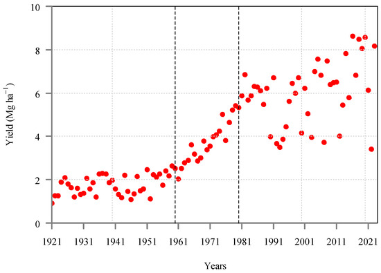
Figure 1. Maize yield in Hungary in the period of 1921–2023 (source: Hungarian Statistical Office [18]). In the period from 1960 to 1980 (between the dashed lines), yield increase followed a nearly linear trend.

The reliability model assumes that the time series exhibits stationary Markov properties. Sufficiently big datasets assure an acceptable level of uncertainty in the estimation. For the period of 1961–1979, the time series did not exhibit stationary Markov properties; hence, they were not involved in the modeling. The test results for the Markov properties of the probability of maize yield failure and high yield by at least 15% and over 30% in the periods of 1925–1960 and 1985–2023 prove that the process is memoryless; the p-values exceed the 0.05 threshold for rejecting the null hypothesis in the case of each yield data sequence (Table 1).

Table 1. Markov properties of the data sequences and probability of maize yield failure or high yield by at least 15% and over 30% in the periods of 1925–1960 and 1985–2023 in Hungary.

Period	Chi-Square		Degree of Freedom		p-Value
	±15%<	±30%<	±15%<	±30%<	±15%<	±30%<
1925–1960	11.10833	5.415921	12	6	0.519658	0.4916765
1985–2023	13.63532	2.611228	12	9	0.3245997	0.977741

All three initial states were observed to converge to the same final state. Hence, the chain was considered ergodic. For a Markov chain to be ergodic means that, in the long run, the chain “forgets its initial state” and always converges to the same stationary distribution. All 12 simulations showed similar behavior; an example is shown in Figure 2.

Figure 2. Results of transition matrix simulation starting with the average state, with differences of 30% for the 1925–1960 period. Dashed lines represent the steady-state values.

3.2. Probability of Maize Yield Failure and High Yield in Hungary in the 1925–1960 Period

Maize yield varied between 0.92 and 2.62 t ha⁻¹ in the period of 1925–1960 in Hungary. Maize yield fluctuation does not seem to show any trends. Differences from the previous five-year moving average by being higher or lower by at least 15% were found to be 22 times more likely, while it was only 9 times more likely for being over ±30% (Figure 3).

Figure 3. Maize yield fluctuation compared to the previous five-year moving average characteristic for the 1925–1960 period (red and blue dashed lines show yield failure or high yield by at least ±15% and over ±30% compared to the five-year moving average (black dashed line), respectively).

Transition matrix results characterizing the fluctuation of maize yield by at least ±15% between 1925 and 1960 are visualized in Figure 4. There are three states, each represented by a vertex of the triangle, where arrows show the transition from one to another. There are nine possible transitions, e.g., the average yield can be followed by high yield or failure, or it can remain near the average in the following year. The probability of transitioning is indicated numerically. The sum of the probabilities given in the figure may differ from 1.00 due to rounding in the figure.

Figure 4. Markov chain plot represented with a transition probability diagram, with at least a ±15% maize yield fluctuation compared to the previous five-year moving average within the 1925–1960 period.

Within the period of 1925–1960, the probability that a year with average yield was followed by another year differing by less than ±15% was 17%, but it increased to 42–42% for having either at least 15% higher yield or yield failure in the following year. When the yield was higher than average by at least 15%, the probability of having a similarly high yield was found to be 23%, while it was 62% to have an average yield next year and 15% to have yield failure by at least 15%. A year with yield failure was found to be followed by another poor year with a probability of 22%, while it was 33% and 44% to have an average or high yield the next year, respectively.

Table 2 summarizes the 95% confidence intervals of the transition probabilities in the case of at least ±15% maize yield fluctuation compared to the previous five-year moving average within the period of 1925–1960.

Table 2. The 95% confidence intervals of the transition probabilities in the case of at least ±15% yield fluctuation, 1925–1960.

		Average	Failure	High
	Average	0	0.051	0.051
Lower endpoint	Failure	0	0	0.008
	High	0.189	0	0
	Average	0.398	0.782	0.782
Upper endpoint	Failure	0.711	0.530	0.879
	High	1	0.367	0.492

The true probability within the 95% confidence interval can be expected to fall within the range of the lower and upper endpoints. The range is strongly dependent on the sample size and variation. Within the assessed period, the very rare states’ confidence intervals are the highest. In considering the steady-state distribution that represents the long-time behavior, in the case of the yield statistical pattern found in the 1925–1960 period, the probability of having average maize yield, yield failure, and high yield would be 37%, 27%, and 36%, respectively.

Transition matrix results characterizing the maize yield fluctuation by over ±30% between 1925 and 1960 are shown in Figure 5. The probability of such an extreme difference for the yield of a year compared to the following year was found to be 76%. Crop yield failure could be expected with 8% probability, and exceptional yield with 16% probability. After a crop yield failure, a year with an average yield can be expected with 50% probability. Failure would occur again with 25% probability, and a high yield with 25% probability. After a high-yield year, an average yield was found to occur with 80% probability and crop failure with 20% probability. During this period, a high yield never occurred after a high yield.

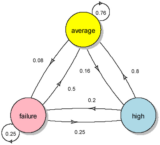
Figure 5. Markov chain plot represented with a transition probability diagram, with over ±30% maize yield fluctuation compared to the previous five-year moving average within the 1925–1960 period.

Table 3 summarizes the 95% confidence intervals of the transition probabilities in the case of at least ±30% maize yield fluctuation compared to the previous five-year moving average within the 1925–1960 period. Similarly to the case of ±15% maize yield fluctuation, the very rare states’ confidence intervals are the highest in this period.

Table 3. The 95% confidence intervals of the transition probabilities in the case of over ±30% yield fluctuation, 1925–1960.

		Average	Failure	High
	Average	0.418	0	0.003
Lower endpoint	Failure	0	0	0
	High	0.016	0	0
	Average	1	0.191	0.317
Upper endpoint	Failure	1	0.739	0.739
	High	1	0.592	0

In considering the long-time behavior, with the statistics of the 1925–1960 data, the probability of average maize yield, yield failure, and high yield would be 73.5%, 11.8%, and 14.7%, respectively.

3.3. Probability of Maize Yield Failure and High Yield in Hungary in the 1985–2023 Period

Maize yield varied between 3.40 and 8.60 t ha⁻¹ in the period of 1985–2023 in Hungary. Maize yield fluctuation does not seem to show any trends. Differences from the previous five-year moving average by being higher or lower by at least 15% were found to be 23 times more likely, while it was 13 times more likely for being over ±30% (Figure 6).

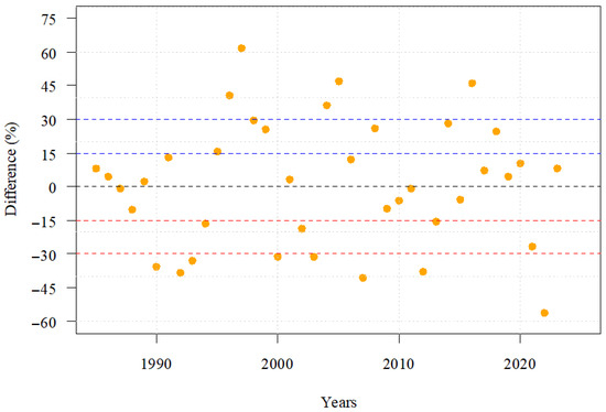
Figure 6. Maize yield fluctuation compared to the previous five-year moving average characteristic for the 1985–2023 period (red and blue dashed lines show yield failure or high yield by at least ±15% and over ±30% compared to the five-year moving average (black dashed line), respectively).

Figure 7 represents the transition matrix results for the yield fluctuation by at least ±15% between 1985 and 2023. After an average harvest, there was a 47% probability of an average harvest again. We could expect a high harvest with 13% probability and 40% probability of crop failure. Years with high harvests were found to repeat with 45% probability, i.e., the phenomenon repeats itself. With 45% probability, an average harvest follows, and with only a 9% probability of crop failure. A year with a low harvest was calculated to repeat with 42% probability, which is quite a high value. Then, with 25% and 33% probability, an average and high harvest would be expected, respectively.

Figure 7. Markov chain plot represented with a transition probability diagram, with at least ±15% maize yield fluctuation compared to the previous five-year moving average within the 1985–2023 period.

Table 4 summarizes the 95% confidence intervals of the transition probabilities in the case of at least ±15% maize yield fluctuation compared to the previous five-year moving average within the 1985–2023 period. Similarly to the 1925–1960 period, the very rare states’ confidence intervals are the highest.

Table 4. The 95% confidence intervals of the transition probabilities in the case of at least ±15% yield fluctuation, 1985–2023.

		Average	Failure	High
	Average	0.121	0.079	0
Lower endpoint	Failure	0	0.05	0.007
	High	0.056	0	0.056
	Average	0.812	0.400	0.133
Upper endpoint	Failure	0.533	0.782	0.659
	High	0.853	0.269	0.853

Based on the long-term steady state, the probability of average harvest, high harvest, and crop failure would be 39.5%, 29%, and 31.5%, respectively.

Figure 8 presents the transitions matrix results for yield fluctuation by over ±30% between 1985 and 2023. After an average harvest, there was a 64% probability of an average harvest again. We could expect crop failure with 28% probability, and high harvest with only 8% probability. The probability of a high-harvest year recurring was 40%. An average harvest could be expected with 60% probability. The probability of crop failure after a high-harvest year was zero. This did not occur in the period under review. After crop failure, a 12% probability of another crop failure was calculated. We could expect a high harvest with 12% probability and a year with an average harvest with 70% probability.

Figure 8. Markov chain plot presented with a transition probability diagram, with over ±30% maize yield fluctuation compared to the previous five-year moving average within the 1985–2023 period.

Table 5 summarizes the 95% confidence intervals of the transition probabilities in the case of over 30% maize yield fluctuation compared to the previous five-year moving average within the 1985–2023 period. Similarly to the 1925–1960 period, the very rare states’ confidence intervals are the highest.

Table 5. The 95% confidence interval of the transition probabilities in the case of over ±30% yield fluctuation, 1985–2023.

		Average	Failure	High
	Average	0.326	0.073	0
Lower endpoint	Failure	0.149	0	0
	High	0	0	0
	Average	0.954	0.487	0.191
Upper endpoint	Failure	1	0.369	0.369
	High	1	0	0.954

Based on the steady state, the probability of average harvest, crop failure, and high harvest would be 66%, 21%, and 13%, respectively.

4. Discussion

The effects of weather extremes on crop failure are significant. The probability of variation in crop yield tends to increase. Today, yields under optimal conditions are close to the genetic potential compared to the earlier performance. Thus, any adverse effect results in higher loss; high yield assumes intensive utilization of resources with increased sensitivity for any shortage. Furthermore, when drought and heat stress occur together, they can lead to a higher probability of crop damage compared to when these stressors occur individually (e.g., [19]). Studies suggest that current maize models may not adequately capture the impact of climate extremes, specifically heat and drought, on maize photosynthesis and yield (e.g., [20]). According to Shi and Tao [21], in the African continent, for each 1 °C increase in mean temperature, yield losses were over 10% in eight countries and between 5 and 10% in ten countries. A 10% decrease in average precipitation led to more than a 5% decrease in yields in 20 countries. A decrease of 0.5 in the standardized precipitation evapotranspiration index (SPEI) resulted in over 30% losses of maize yields in 32 countries. Obour et al. [22] studied the primary causes of maize production failure with the conclusion that factors such as poor soil quality, inadequate farm inputs, and under-resourced mechanization had a lesser impact on maize production failure than drought conditions unfavorable for maize growth. Regarding Hungary, annual precipitation has not changed within the last 100 years; however, since 2000, it has shown increasing variation in distribution over the years, with shortage typically in the vegetation period. Annual average temperature, however, has increased in the last 25 years, resulting in an increase in potential evapotranspiration [23]. Heat stress has occurred after 2000 too. It must be noted that without taking technological development into consideration, prediction models may overestimate the adverse effect of climate change on crop production [24]. Srivastava et al. [25] established that yield fluctuations are reflected through the variability in simulated maize yields when using different sets of climate data for regional simulations. They found that there was less variability in the simulated yield when using a consistent dataset from the same source. In contrast, when using a combined dataset from different sources, the variability was higher, indicating that the choice of climate data source can introduce significant uncertainties into crop simulation results.

In our study, based on the maximum likelihood estimation, in the 1925–1960 period, the probability of occurrence of average maize yield or higher by at least 15% was found to be the highest for the investigated region, Hungary, while that of failure by at least 15% was found to be 27%. Interestingly, when considering at least a 15% difference from the previous five-year moving average, the probability of failure was calculated to be higher, while that of the high yield was lower for the 1985–2023 period (Table 6).

Table 6. Transition matrices for maize yield in the 1925–1960 and 1985–2023 periods in Hungary. Yield failure and high yield are considered with the probability of being lower and higher than the moving average by at least 15%. The steady-state distribution characteristics for long-term maize yield are indicated in bold.

Period		Average	Failure	High
	Average	0.166	0.417	0.417
	Failure	0.333	0.222	0.445
1925–1960	High	0.615	0.154	0.231
	Steady state	0.372	0.270	0.358
	Average	0.467	0.400	0.133
	Failure	0.250	0.417	0.333
1985–2023	High	0.454	0.091	0.455
	Steady state	0.395	0.316	0.289

In conclusion, with the consideration of maize yield variation by at least ±15%, the three states occurred with similar probabilities in the past four decades. Thus, we found 15% as a threshold to be improper for the analysis of the phenomenon and inadequate for making probability estimations for the near future.

When we define maize yield variation as high in the case of the threshold ±30%, the probability of average-harvest years increases (Table 7). Any state returns to the average with high probability, which represents regression and suggests normal distribution. This assures the crowd consistency and stability; hence the property of concern remains characteristic in the long term.

Table 7. Transition matrices for maize yield in the 1925–1960 and 1985–2023 periods in Hungary. Yield failure and high yield are considered with the probability of being lower and higher than the moving average by over 30%. Steady-state distribution characteristics for long-term maize yield are indicated in bold.

Period		Average	Failure	High
	Average	0.760	0.080	0.160
	Failure	0.500	0.250	0.250
1925–1960	High	0.800	0.200	0.000
	Steady state	0.735	0.118	0.147
	Average	0.640	0.280	0.080
	Failure	0.75	0.125	0.125
1985–2023	High	0.600	0.000	0.400
	Steady state	0.658	0.210	0.132

In comparing the probability of yield failure calculated for the 1925–1960 period with that of the 1985–2023 period, long-term tendency shows duplication; specifically, the frequency of maize yield failure increased from 11.8% to 21%. At the same time, the probability of average yield and high yield moderately decreased. Yield variation is dominant in the negative range.

Technological development aims to increase crop performance under optimal conditions; however, higher genetic potential occurs in conjunction with higher sensitivity to environmental extremes. For example, without properly adjusting irrigation to the actual water demand of crops, as well as promoting land drainage, both water shortage and excess are by far the most determinative weather factors for farmers in the investigated region [26]. In Hungary, crops with high genetic potential are produced, and nutrition and crop protection are of a high standard. The size of the irrigated area, however, will be expanded to 20% of arable land by 2030.

Process-based models that incorporate mechanistic understanding of physiological, meteorological, and edaphic factors affecting yield, remain essential for mechanistic yield forecasting incorporating weather extremes. Our methodology offers a complementary probabilistic perspective focusing on yield fluctuation dynamics over time as a stochastic process. Discrete Markov chain approach circumvents some assumptions and data requirements, offering an alternative that specifically targets yield variability transitions as a stochastic time series problem. Similar Markovian methodologies have been applied effectively in crop condition forecasting and drought risk assessment [7,12], supporting the broader value of Markov models for agricultural risk characterization.

5. Conclusions

Towards our goals, we established the following: (1) The probability of maize yield variability for the examined periods can be modeled using the Markov chain method. This was proven by performing Chi-square tests in series. As the degree of yield fluctuation increases, the probability of average-yield years increases. (2) In the 1925–1960 period, considering both degrees of yield fluctuation, average and high yields occurred with the highest probability; the fluctuation of 30% gave the clearest results. This changed in the 1985–2023 period, as the probability of crop failure increased and the probability of average and high yields decreased. (3) Technological development has advanced in recent decades, but the adverse effects of climate change have increased the probability of crop failure. Currently, we cannot mitigate the adverse effects of weather using existing technologies. If climate change continues, according to the trend of recent decades, we will be forced to change current practices in order to reduce the frequency of crop failure. The study results regarding the 30% fluctuation can inform ministries and specialists in their work and provide an opportunity to mitigate the adverse effects of extreme crop failure.

The Markov chain method has been mostly applied for weather data analyses in relation to agriculture and climate change. The adaptability of such robust models with relatively low data input needs to be tested, as overparametrized chaotic models show a fan effect. Inputting more parameters in the model does not necessarily yield more reliable results.

This study demonstrates the applicability of the discrete-time Markov chain method for assessing inter-annual crop yield stability and risk under observed historical variability, as well. The approach is not a deterministic, process-based forecast of crop yield. It assumes a first-order, time-homogeneous Markov process based on regional historical yield data, not considering meteorological drivers (e.g., drought, heat stress), soil parameters, or agronomic adaptations (e.g., management practices, irrigation, cultivar choice). Despite these simplifications, the method provides an informative probabilistic risk profile of yield variability across years.

References

- Kulinich, M.; Fan, Y.; Penev, S.; Evans, J.P.; Olson, R. A Markov chain method for weighting climate model ensembles. Geosci. Model Dev. 2021, 14, 3539–3551. [Google Scholar] [CrossRef]
- Azizah, A.; Welastika, R.; Falah, A.N.; Ruchjana, B.N.; Abdullah, A.S. An Application of Markov Chain for Predicting Rainfall Data at West Java Using Data Mining Approach. IOP Conference Series: Earth Environ. Sci. 2019, 303, 012026. [Google Scholar] [CrossRef]
- Pope, E.C.D.; Stephenson, D.B.; Jackson, D.R. An adaptive Markov Chain approach for probabilistic forecasting of categorical events. Mon. Weather Rev. 2020, 148, 3681–3691. [Google Scholar] [CrossRef]
- Lennartsson, J.; Baxevani, A.; Chen, D. Modelling Precipitation in Sweden using multiple step markov chains and a composite model. J. Hydrol. 2008, 363, 42–59. [Google Scholar] [CrossRef]
- Gidey, E.; Dikinya, O.; Sebego, R.; Segosebe, E.; Zenebe, A. Cellular automata and Markov Chain (CA-Markov) model-based predictions of future land use and land cover scenarios (2015–2033) in Raya, northern Ethiopia. Model. Earth Syst. Environ. 2017, 3, 1245–1262. [Google Scholar] [CrossRef]
- Beroho, M.; Briak, H.; Cherif, E.F.; Boulahfa, I.; Ouallali, A.; Mrabet, R.; Kebede, F.; Bernardino, A.; Aboumaria, K. Future Scenarios of Land Use/Land Cover (LULC) Based on a CA-Markov Simulation Model: Case of a Mediterranean Watershed in Morocco. Remote Sens. 2023, 15, 1162. [Google Scholar] [CrossRef]
- Fadhil, R.M.; Unami, K. A multi-state Markov chain model to assess drought risks in rainfed agriculture: A case study in the Nineveh Plains of Northern Iraq. Stoch. Environ. Res. Risk Assess. 2021, 35, 1931–1951. [Google Scholar] [CrossRef]
- Kemsley, W.S.; Osborn, T.J.; Dorling, S.R.; Wallace, C.; Parker, J. Selecting Markov chain orders for generating daily precipitation series across different Köppen climate regimes. Int. J. Climatol. 2021, 41, 6223–6237. [Google Scholar] [CrossRef]
- Solonen, A.; Ollinaho, P.; Laine, M.; Haario, H.; Tamminen, J.; Järvinen, H. Efficient MCMC for Climate Model Parameter Estimation: Parallel Adaptive Chains and Early Rejection. Bayesian Anal. 2012, 7, 715–736. [Google Scholar] [CrossRef]
- Tariq, A.; Shu, H. CA-Markov Chain Analysis of Seasonal Land Surface Temperature and Land Use Land Cover Change Using Optical Multi-Temporal Satellite Data of Faisalabad, Pakistan. Remote Sens. 2020, 12, 3402. [Google Scholar] [CrossRef]
- Matis, J.H.; Saito, T.; Grant, W.E.; Iwig, W.C.; Ritchie, J.T. A Markov chain approach to crop yield forecasting. Agric. Syst. 1985, 18, 171–187. [Google Scholar] [CrossRef]
- Stokes, J.R. A Markov chain model of crop conditions and intrayear crop yield forecasting. J. Forecast. 2024, 43, 583–592. [Google Scholar] [CrossRef]
- Al-Ani, L.A.F.; Alhiyali, A.D.K. Using Markov Chains to Predict Productivity of Maize in Iraq for the Period (2019–2025). Appl. Econ. Financ. 2021, 8. [Google Scholar] [CrossRef]
- Huang, H.; Huang, J.; Wu, Y. Markov Chain Monte Carlo and Four-Dimensional Variational Approach Based Winter Wheat Yield Estimation. In Proceedings of the IGARSS 2020—2020 IEEE International Geoscience and Remote Sensing Symposium, Waikoloa, HI, USA, 26 September–2 October 2020; pp. 5290–5293. [Google Scholar] [CrossRef]
- Chang, Y.; Latham, J.; Licht, M.; Wang, L. A data-driven crop model for maize yield prediction. Commun. Biol. 2023, 6, 439. [Google Scholar] [CrossRef]
- Huzsvai, L.; Juhász, C.; Seddik, L.; Kovács, G.; Zsembeli, J. The Future Probability of Winter Wheat and Maize Yield Failure in Hungary Based on Long-Term Temporal Patterns. Sustainability 2024, 16, 3962. [Google Scholar] [CrossRef]
- Spedicato, G. Discrete Time Markov Chains with R. R J. 2017, 9, 84–104. [Google Scholar] [CrossRef]
- Hungarian Statistical Office. Available online: https://www.ksh.hu/stadat_eng (accessed on 1 December 2024).
- Ribeiro, A.F.S.; Russo, A.; Gouveia, C.M.; Páscoa, P.; Zscheischler, J. Risk of crop failure due to compound dry and hot extremes estimated with nested copulas. Biogeosciences 2020, 17, 4815–4830. [Google Scholar] [CrossRef]
- Jin, Z.; Zhuang, Q.; Tan, Z.; Dukes, J.S.; Zheng, B.; Melillo, J.M. Do maize models capture the impacts of heat and drought stresses on yield? Using algorithm ensembles to identify successful approaches. Glob. Change Biol. 2016, 22, 3112–3126. [Google Scholar] [CrossRef] [PubMed]
- Shi, W.; Tao, F. Vulnerability of African maize yield to climate change and variability during 1961–2010. Food Secur. 2014, 6, 471–481. [Google Scholar] [CrossRef]
- Obour, P.B.; Arthur, I.K.; Owusu, K. The 2020 Maize Production Failure in Ghana: A Case Study of Ejura-Sekyedumase Municipality. Sustainability 2022, 14, 3514. [Google Scholar] [CrossRef]
- Huzsvai, L.; Zsembeli, J.; Kovács, E.; Juhász, C. Response of winter wheat (Triticum aestivum L.) yield to the increasing weather fluctuations in a continental region of four-season climate. Atmosphere 2022, 12, 314. [Google Scholar] [CrossRef]
- Huzsvai, L.; Zsembeli, J.; Kovács, E.; Juhász, C. Can technological development compensate for the unfavorable impacts of climate change? Conclusions from 50 years of maize (Zea mays L.) production in Hungary. Clim. Change Agrometeorol. Time Ser. 2020, 11, 1350. [Google Scholar] [CrossRef]
- Srivastava, A.K.; Ceglar, A.; Zeng, W.; Gaiser, T.; Mboh, C.M.; Ewert, F. The Implication of Different Sets of Climate Variables on Regional Maize Yield Simulations. Atmosphere 2020, 11, 180. [Google Scholar] [CrossRef]
- Juhász, C.; Gálya, B.; Kovács, E.; Nagy, A.; Tamás, J.; Huzsvai, L. Seasonal predictability of weather and crop yield in regions of Central European continental climate. Comput. Electron. Agric. 2020, 173, 105400. [Google Scholar] [CrossRef]
Disclaimer/Publisher’s Note: The statements, opinions and data contained in all publications are solely those of the individual author(s) and contributor(s) and not of MDPI and/or the editor(s). MDPI and/or the editor(s) disclaim responsibility for any injury to people or property resulting from any ideas, methods, instructions or products referred to in the content. |
© 2025 by the authors. Licensee MDPI, Basel, Switzerland. This article is an open access article distributed under the terms and conditions of the Creative Commons Attribution (CC BY) license (https://creativecommons.org/licenses/by/4.0/).