UFORE-D Modeling of Urban Tree Influence on Particulate Matter Concentrations in a High-Altitude Latin American Megacity

Abstract

Urban trees reduce particulate matter (PM) concentrations through dry deposition, interception, and modifying wind patterns, improving air quality and saving public health expenses in urban planning. The main objective of this article is to present an analysis of the influence of urban trees on PM₁₀ and PM_2.5 concentrations in a high-altitude Latin American megacity (Bogotá, Colombia) using UFORE-D modeling. Six PM monitoring stations distributed throughout the megacity were used. Hourly climatic and PM data were collected for seven years, along with dendrometric and cartographic analyses within 200 m of the monitoring stations. Land cover was quantified using satellite imagery (Landsat 8) in order to perform a spatial analysis. The results showed that the UFORE-D model effectively quantified urban forest canopy area (CA) impact on PM₁₀ and PM_2.5 removal, showing strong correlations (R² = 0.987 and 0.918). PM removal increased with both CA and ambient pollutant concentrations, with CA exhibiting greater influence. Sensitivity analysis highlighted enhanced air quality with increased leaf area index (LAI: 2–4 m²/m²), particularly at higher wind speeds. PM₁₀ removal (1.05 ± 0.01%) per unit CA exceeded PM_2.5 (0.71 ± 0.09%), potentially due to resuspension modeling. Model validation confirmed reliability across urban settings, emphasizing its utility in urban planning. Scenario analysis (E1–E4, CA: 8.30–95.4%) demonstrated a consistent positive correlation between CA and PM removal, with diminishing returns at extreme CA levels. Urban spatial constraints suggested integrated green infrastructure solutions. Although increased CA improved PM removal rates, the absolute reduction of pollutants remained limited, suggesting comprehensive emission monitoring.

1. Introduction

Air quality in urban environments has become one of the most significant challenges for governments in recent decades due to the effects on public health, the environment, and the economy caused by high concentrations of particulate matter (PM). Studies reported a strong correlation between the incidence of respiratory and cardiovascular diseases and the increase in PM concentrations [1,2]. This issue, driven by the aforementioned correlation, intensified in densely populated human settlements [3], particularly in megacities [4,5]. Urban environments most affected by high PM concentrations were those with deficient mitigation strategies. For example, this was possibly the case for the megacities of Kolkata in India and Beijing, Chengdu, and Shanghai in China. In these megacities, the extraction of natural resources and unsustainable combustion practices significantly impacted both the environment and public health [6,7,8]. In Latin America, for example, it was reported that, in 2019, about 95% of the population in megacities and growing cities exceeded the World Health Organization guidelines for PM_2.5 [9]. The main influencing factors identified were high population density, deficient public transportation systems, abundant road intersections, high motorization rates, and a high GDP per capita [10,11]. Therefore, it was necessary to better understand the dynamics of PM under different urban contexts, including high-altitude Latin American megacities, where information was still limited.

Multiple studies described the effect of urban trees on PM concentrations. Some studies reported an inverse relationship between increased tree cover and PM concentrations [12,13]. Urban trees captured PM through various mechanisms. Dry deposition, where particles adhered to the surfaces of leaves and stems, was a key process influenced by tree species and canopy structure [14,15]. Interception, where leaves acted as physical barriers, was more effective in areas with high tree density [16]. Trichomes and waxy surfaces of some species also contributed to PM capture [17]. Rain washed away accumulated particles, and trees modified PM dispersion and dilution by altering wind patterns [18]. The reduction in air temperature by trees also decreased the formation of secondary aerosols [19]. The use of tree covers to improve urban air quality was so promising that McDonald et al. [20] specifically indicated where trees should be planted for greater PM retention within the framework of urban planning in the United Kingdom. This improved the quality of life for residents and represented savings in public health-related expenses. Kroeger et al. [21] also reported that strategically locating trees in 27 U.S. cities could save up to USD 102 million annually in public health expenses due to this ecosystem service.

However, studies modeling the effect of tree cover on air quality in high-altitude megacities in developing countries were still scarce. These megacities had particular climatic, geographic, and socioeconomic characteristics that could influence PM dynamics. Bogotá (Colombia), at 2640 m above sea level, had a cold, variable climate with high solar radiation and low humidity. Rainfall was bimodal, and frosts were frequent [22,23]. The city’s mountainous surroundings and flat topography influenced pollutant dispersion and accumulation [24]. As an economic center with high population density, Bogotá faced air quality challenges due to traffic congestion and industrial activity. Socioeconomic inequality affected pollution exposure, especially in low-income areas [25]. All of the above constituted, in part, one of the main motivations for conducting this study.

There were different methodological approaches to simulate the influence of trees on urban air quality. These approaches were divided into two main categories: (1) those that used indirect variables to estimate the removal of air pollutants by trees (indirect approach); (2) those that directly determined removal values through in situ measurements (direct approach) [26,27]. Within the indirect approach, one of the most widely used methodologies was UFORE (Urban Forest Effects Model) [28]. This methodology was also used by Hirabayashi et al. [29] and Nowak et al. [30] for the development of the i-Tree computational tool. This methodology was based on a mathematical model that related climatic conditions, PM concentrations, and dendrometric variables to determine the PM retention capacity of trees in a given area [31]. Another indirect methodology used was remote sensing, which involved characterizing green areas, climatic conditions, and air quality to determine the retention capacity of urban trees. For example, this methodology was used in Seoul (South Korea) with MODIS (Moderate Resolution Imaging Spectroradiometer) images, where, by varying the analysis zones (radius between 300 and 1000 m), and monitoring stations, it was determined that areas with larger urban forests showed the lowest air pollution indices (PM₁₀ = −5.30%; PM_2.5 = −4.80%) [32]. This methodology was also replicated by Zhao et al. [33] to study the temporal correlation between buffer areas (vegetation cover or wetlands) and PM concentrations. These authors considered the temporal variation of land cover and climatic variables.

The UFORE methodology considered various criteria to study the influence of trees on PM concentrations. Firstly, it collected detailed tree information, including species, diameter, height, canopy cover, density, and spatial distribution. This information allowed for the characterization of the tree structure and its capacity to intercept and capture atmospheric particles. Secondly, UFORE incorporated climatological information, such as wind speed and direction, temperature, humidity, precipitation, and solar radiation. These variables influenced the dispersion and deposition of PM, as well as the trees’ capacity to capture it [34]. Moreover, the methodology required air quality information, specifically PM₁₀ and PM_2.5 concentrations, and other relevant air pollutants [35]. UFORE also considered emission information from sources such as vehicular traffic and industries, which were fundamental for modeling the dispersion and impact of PM in the study area [36]. With this information, UFORE used deposition models to estimate the amount of PM captured by trees through dry deposition, one of the main removal mechanisms. Other effects, such as particle interception and air temperature reduction, were also estimated [37]. Lastly, UFORE analyzed the results to quantify the benefits of trees in terms of PM concentration reduction and other ecosystem services [38].

Numerous studies in developed nations and Asian megacities have documented the PM capture capabilities of urban trees using indirect modeling approaches like UFORE and direct in situ measurements. However, these studies focused on temperate or subtropical climates and different socioeconomic conditions. Consequently, the applicability and performance of models like UFORE remained unexplored in high-altitude urban centers such as Bogotá. This research gap left planners and policymakers with limited guidance on using urban forestry for air quality management, highlighting the need for context-specific investigations.

The main objective of this article is to present an analysis of the influence of urban trees on PM₁₀ and PM_2.5 concentrations in a high-altitude Latin American megacity (Bogotá, Colombia) using UFORE-D modeling. This study uses six PM monitoring stations distributed throughout the megacity. The analysis of the influence of trees on PM concentrations is conducted in the areas influenced by these monitoring stations. This study was relevant in the context of air quality in high-altitude megacities for the following aspects: (i) deepening the understanding of the PM retention capacity of urban trees under high-altitude climatic conditions; (ii) analyzing the performance of UFORE-D modeling in the study context (population, climatic, and economic); (iii) establishing possible modeling scenarios for improving air quality through urban trees.

2. Materials and Methods

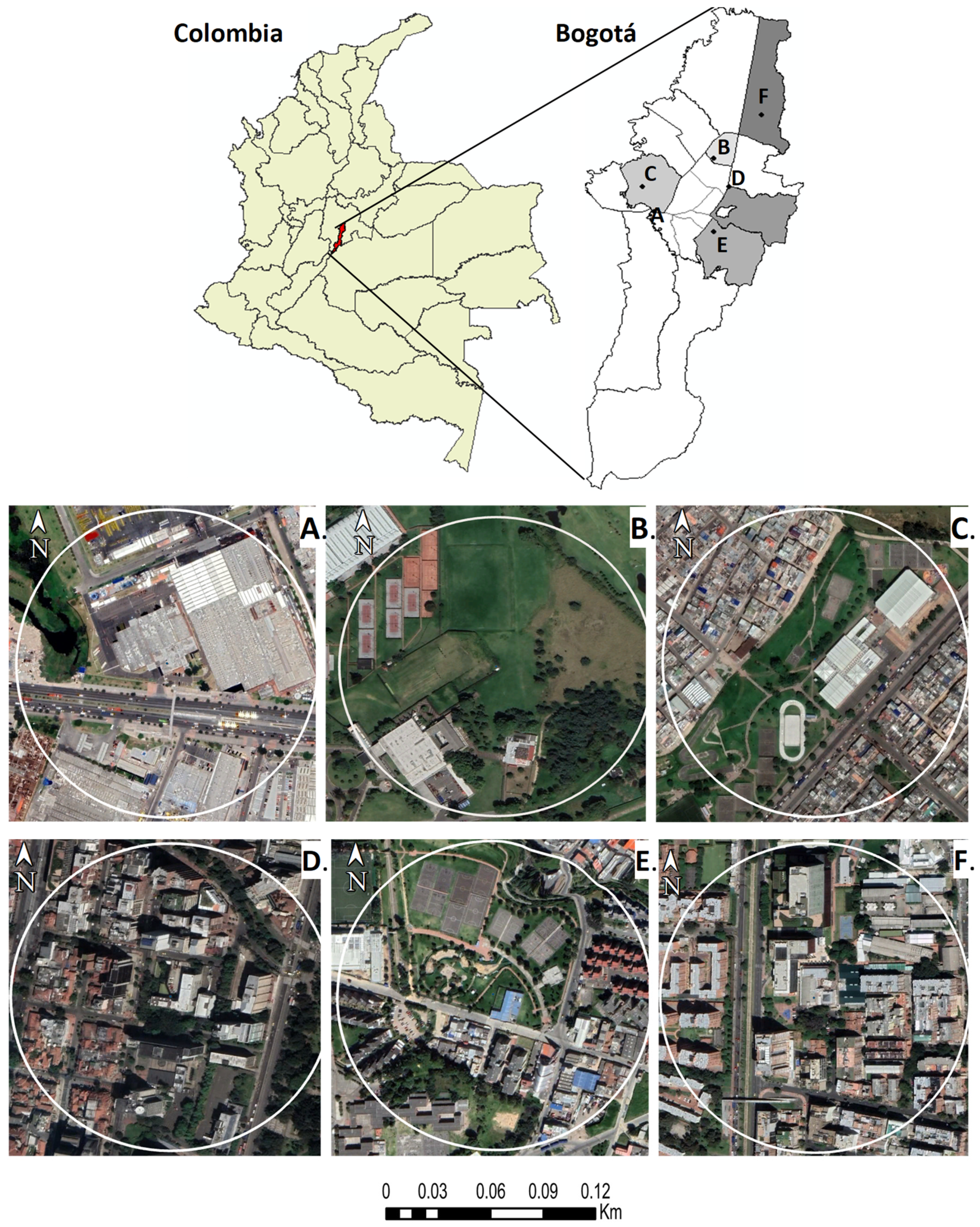
2.1. Description of the Study Site

Six air quality monitoring stations were established based on their representativeness in surface coverage, land cover, tree density, and historical information on PM_2.5 and PM₁₀ concentrations in the megacity under study. These monitoring stations were located throughout the megacity and were identified as follows: Carvajal—Sevillana = CSE, Centro de Alto Rendimiento = CAR, Kennedy = KEN, MinAmbiente = MIN, San Cristóbal = SCR, and Usaquén = USQ (Figure 1). The analysis influence radius considered in this study was 200 m, in relation to the physical location of each established monitoring station. The climate of the megacity was tropical mountain (cold climate), with an average annual temperature between 13.3 and 14.3 °C, and hourly temperature variations between 7.20 and 19.0 °C (daily range up to 13 °C). The average altitude of the monitoring stations was 2599 m above sea level. These stations were also equipped to measure temperature, precipitation, solar radiation, relative humidity, and wind speed and direction.

Table 1. Main characteristics of the study sites according to the established monitoring stations.

Characteristics		CSE	CAR	KEN	USQ	SCR	MIN
Location	Lat. (N)	4°35′44.2″	4°39′30.5″	4°37′30.2″	4°42′37.3″	4°34′21.1″	4°37′31.8″
	Long. (W)	74°8′54.9″	74°5′2.3″	74°9′40.8″	74°1′49.5″	74°5′1.7″	74°4′1.1″
	Alt. (masl)	2563	2577	2580	2570	2688	2621
	GH (m)	3.00	0.00	3.00	10.0	0.00	15.0
	ZT	Urban	Urban	Urban	Urban	Urban	Urban
	ST	Traffic/Industrial	Background	Background	Background	Background	Traffic
	SL	Rooftop	Green zone	Green zone	Rooftop	Green zone	Rooftop
	SPH (m)	4.20	4.05	7.71	16.5	4.88	4.67
	WSH (m)	13.0	10.0	10.0	19.0	10.0	19.0
Land cover	Impermeable (%)	80.2	19.1	66.9	80.6	53.6	81.3
	Vegetation (%)	16.5	65.9	25.9	19.4	42.4	18.7
	Water body (%)	1.60	0.00	0.00	0.00	0.00	0.00
	Uncovered land (%)	1.80	15.0	0.00	0.00	3.93	0.00
Urban trees	Trees by locality	36,045	36,245	129,241	120,279	65,813	56,433
	Trees per inhabitant	0.05	0.253	0.125	0.213	0.166	0.334
	Trees per hectare	18.65	30.47	35.84	35.76	40.4	51.61
Air pollutants	PM10 (μg/m3)	78.9	32.6	64.9	37.2	31.9	38.0
	PM2.5 (μg/m3)	30.6	17.9	28.3	13.1	10.8	16.6
Climatology	WS (m/s)	1.36	1.25	2.34	1.57	1.54	1.24
	WD (°)	175	191	190	143	128	162
	T (°C)	15.9	15.1	16.4	14.7	13.7	-
	P (mm)	755	995	1012	954	1014	801
	SR (W/m2)	-	151	165	-	217	-
	RH (%)	-	66.0	61.0	-	67.0	-

Note: Lat. = Latitude (N), Long. = Longitude (W), Alt. = Altitude, GH = Ground Height, ZT = Zone Type, ST = Station Type, SL = Sample Location, SPH = Sample Point Height, WSH = Wind Sensor Height, PM₁₀ = Particulate Matter ≤ 10 µm, PM_2.5 = Particulate matter ≤ 2.5 µm, WS = Average wind speed, WD = Average wind direction, T = Average temperature, P = Average annual precipitation, SR = Average cumulative solar radiation, and RH = Average relative humidity.

shows the main characteristics of each of the monitoring stations considered.

2.2. Information Collection

In this study, hourly data were continuously collected over a seven-year period. The collected data included the following climate and air pollution variables: precipitation (mm), temperature (°C), wind speed (m/s), wind direction, relative humidity (%), solar radiation (W/m²), and PM_2.5 (µg/m³) and PM₁₀ (µg/m³) concentrations. PM was measured using beta attenuation monitors, following the guidelines established by the U.S. Environmental Protection Agency (EPA-454/R-00-039) [39]. The precision of the instruments used for PM was approximately 6.25% for concentrations ≤ 80 µg/m³ and 7.0% for concentrations ≥ 80 µg/m³. This climate and air pollution data were available on the Bogotá Air Quality Monitoring Network platform—RMCAB http://rmcab.ambientebogota.gov.co/home/map (accessed on 1 February 2023). Moreover, dendrometric information was collected for the trees located within the influence areas of each monitoring station (radius = 200 m). The dendrometric variables considered were canopy height, canopy diameter, diameter at breast height, total height, and trunk height [40]. The trees were also georeferenced using the Bogotá Botanical Garden platform—JBB http://sigau.jbb.gov.co/SigauJBB/VisorPublico/VisorPublico (accessed on 1 February 2023). Cartographic information was collected from freely accessible satellite images (Landsat 8) using the Google Earth Pro V.7.3.4.8573 tool [41]. This cartographic information was processed at a spatial resolution of 15 × 15 m², a digital resolution of 4800 × 2220 pixels, and a scale of 1:3600 using ArcGIS V.10.8 software [42]. In selecting the satellite images, it was verified that the cloud cover percentage was null or very low to minimize atmospheric noise [43]. With this cartography, the following land cover types were detected and quantified at each monitoring station [44,45]: impervious (buildings and roads), pervious (vegetation), bare soil, and water bodies.

2.3. Information Analysis

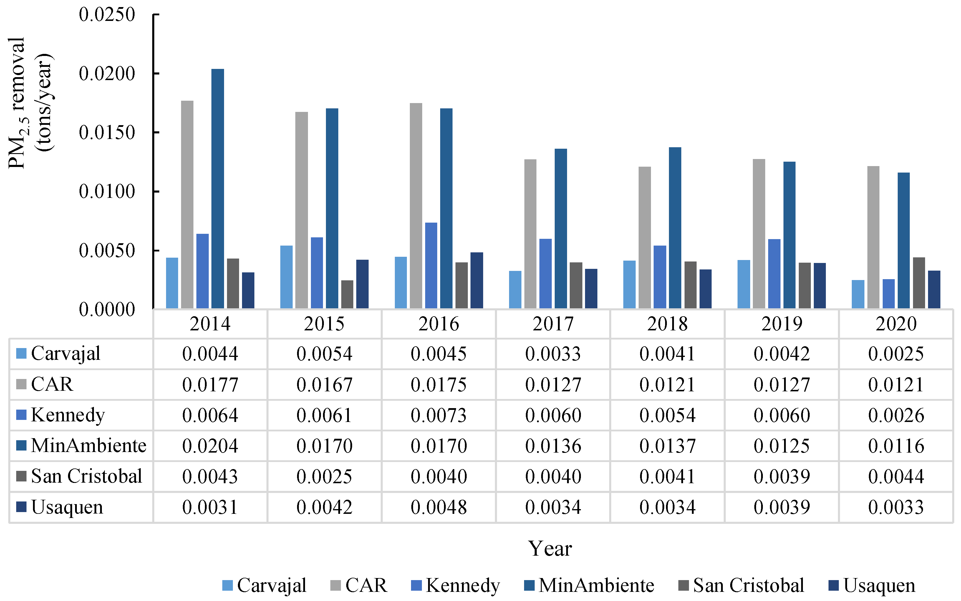
The analysis of the information consisted of four phases. In the first phase, missing data from the time series of climate variables and air pollutants were completed. In this study, all time series had more than 85% of the information during the study period. To complete the missing data, the methods of nearest neighbor [46], normal ratio [47], and autoregressive integrated moving average (ARIMA) time series [48] were used. Two methods were used to complete the information on PM₁₀ and PM_2.5 concentrations. The nearest neighbor method was used when there was only one missing data point. This method inferred the missing data based on an average of the immediately preceding and following data points [49]. The second method, normal ratio, was used considering two or more nearby monitoring stations. Initially, the non-normality of the PM₁₀ and PM_2.5 concentration time series was determined at each monitoring station using the Kolmogorov-Smirnov test (p > 0.05). Subsequently, the Spearman correlation coefficient (rs) was used to determine which nearby monitoring stations had an rs > 0.75. With the stations that met the above selection criteria, the missing data were determined using the normal ratio method [50]. Missing data in the time series of temperature and precipitation, as well as wind speed, wind direction, relative humidity, and solar radiation, were completed using ARIMA time series methods [48] and the nearest neighbor method [46], respectively. Lastly, the homogeneity of the climate variable time series was verified using the double mass curve method [51]. All the above analyses were performed using SPSS V.25 software and Microsoft Excel with 95% confidence.

In the second phase, dendrometric variables of urban trees such as canopy height, canopy diameter, diameter at breast height, total height, and trunk height were analyzed [40] (File S1: LAIs.xlsx). For each tree species, the canopy geometry was analyzed according to the guidelines of the Bogotá vegetation cover manual, which classified them into the following types: sphere, hemisphere, parabola, and cone [52]. Moreover, the canopy surface area (m²) was calculated according to the type of geometry based on the equations reported by Gadow et al. [53], Bataineh and Childs [54], and Burkhart et al. [55]. These equations considered the canopy height and canopy diameter of the tree species. This information was relevant to finally determine the urban tree cover (CA, in %).

In the third phase, the methodology used by the UFORE-D model [29] was applied. In this study, we proceeded to design our own modeling spreadsheet using Microsoft Excel software V.16 (File S2: UFORE-D-PM_2.5.xlsx and File S3: UFORE-D-PM₁₀.xlsx). This model described the phenomenon of PM removal by trees based on the following main variables: precipitation, wind speed, mixing layer height, leaf area index (LAI), canopy projection (Pc), and PM concentration. The average LAIs considered for the trees at each monitoring station were as follows: 3.10 m²/m² (CAR), 2.86 m²/m² (CSE), 2.82 m²/m² (SCR), 2.78 m²/m² (MIN), and 2.75 m²/m² (USQ and KEN) (file in Supplementary Material: LAIs.xlsx). These LAIs were obtained from the Bogotá Botanical Garden platform—JBB http://sigau.jbb.gov.co/SigauJBB/VisorPublico/VisorPublico (accessed on 1 February 2023). The model allowed for the determination of the tons of PM removed by urban trees in a specific time and space. The simulation time scale considered in this study was annual, and the simulation spatial scale corresponded to the area of influence of each monitoring station (circle with a radius of 200 m). A sensitivity analysis was also performed to determine the logic of the model and its behavior using the graphical method. The sensitivity analysis of the model was conducted by constructing relationship graphs between input and output variables using Microsoft Excel software, in which regression models between these variables were obtained. Standardized coefficients (beta coefficients) were also determined to compare the relative strength of the association of each independent variable with the dependent variable [56]. The input (independent) variables considered by the model were as follows: PM₁₀ and PM_2.5 concentrations (µg/m³), LAI (m²/m²), CA (%), and Pc (m²). The output (dependent) variables of interest were PM removal (tons/year) and the annual improvement percentage in air quality (%). As a preliminary step to using the model, test simulations were performed, and the results were compared with those reported by reference international literature [34,36,57,58]. This allowed for the validation of the results obtained through the application of the UFORE-D model.

In the fourth phase, scenarios between PM concentrations and the main characteristics of urban trees considered in this study were modeled. The following tree characteristics were varied in each simulation scenario: LAI and CA. Four simulation scenarios were considered (E1, E2, E3, and E4;

Table 2. Characteristics of the simulation scenarios considered. CAR (CA = 65.9%) and CSE (CA = 16.5%) monitoring stations.

N.	Scenario	CAR			CSE
		CA		LAI	CA		LAI
		(m2)	(%)	(m2/m2)	(m2)	(%)	(m2/m2)
E1	Decline	10,376	8.30	2.00	1211	1.00	2.00
E2	Reference	14,989	11.9	3.10	1677	1.30	2.86
E3	Increase	17,762	14.1	4.00	1947	1.60	4.00
E4	Brooklyn	119,918	95.40	4.00	12,266	9.80	4.00

Note: CA = Tree cover and LAI = Leaf Area Index.

). The scenarios of decrease (E1) and increase (E3) in tree cover were determined based on the annual variation of tree individuals according to the historical inventory of individuals from the Environmental Observatory of Bogotá [59]. The greatest annual decrease and increase in tree individuals were selected for the simulation of scenarios E1 and E3, respectively. In these two scenarios, the lowest and highest LAI were also considered, respectively. The reference scenario (E2) was simulated at the monitoring stations based on the observed (real) conditions of surface cover for the year 2020. The LAI calculated for the reference year was considered in this scenario. Scenario E4, also called Brooklyn, was based on the study developed by Jayasooriya et al. [60]. For this scenario, tree cover values were increased eightfold from the reference scenario (E2) cover. The maximum LAI was also considered for this scenario. This was to simulate a scenario with higher removal values and improvement in urban air quality. At the end of each simulation scenario, PM removal values (tons/year) and PM removal percentages (%) were calculated at each of the monitoring stations considered. In this study, greater attention was paid to the CAR and CSE stations because they had the highest (CA = 65.9%) and lowest (CA = 16.5%) vegetated cover during the reference scenario (E2), respectively. Lastly, the simulated scenarios were cartographically represented for each air pollutant considered (PM₁₀ and PM_2.5).

3. Results

3.1. PM Removal Model

The model was developed under the reference scenario (real conditions), known as E2 (Table 2). Results indicated a direct relationship between urban tree cover (CA, in %) and PM₁₀ removal (tons/year) at the monitoring stations (R² = 0.987). Specifically, the CAR (1.40 Ha of CA) and MIN (1.62 Ha of CA) stations exhibited annual PM₁₀ removal of 0.046 tons and 0.052 tons, respectively (Figure 2). In contrast, the CSE station, with a CA of 0.13 Ha, presented the lowest annual PM₁₀ removal (0.011 tons). Although PM₁₀ concentrations at CAR (21.6 μg/m³) and MIN (20.6 μg/m³) were nearly three times lower than those observed at CSE (63.6 μg/m³), PM₁₀ removal at the latter was four times lower. On average, for all monitoring stations, the annual air quality improvement (PM₁₀) per percentage unit of CA was 1.05 ± 0.01%.

For PM_2.5 modeling, the CAR and MIN stations again showed the highest annual removals (Figure 3), consistent with their higher CA. The average CA at CAR and MIN was 3.39 times greater than at SCR and USQ, and 8.47 times greater than at CSE and KEN. The air quality improvement for PM_2.5, based on CA, was 0.071% for CAR and 0.080% for MIN. The average air quality improvement across all stations was 0.039 ± 0.005%. A strong positive correlation was found between annual PM_2.5 removal and CA (R² = 0.918). Notably, the KEN station, despite high PM_2.5 concentrations (24.9 μg/m³), exhibited an average removal of 0.0057 tons/year. In 2020, with a decrease in PM_2.5 concentrations to 10.7 μg/m³ (−57%), the removal at KEN also decreased to 0.0026 tons/year (−54.4%).

The annual air quality improvement per percentage unit of CA for PM₁₀ was 32.1% higher than for PM_2.5 (0.71 ± 0.09%). The inclusion of PM_2.5 resuspension in the modeling likely contributed to this difference, resulting in lower calculated removals and consequently lower air quality improvement for PM_2.5 compared to PM₁₀. The KEN (0.91%) and CSE (0.81%) stations exhibited the highest annual air quality improvements per percentage unit of CA for PM_2.5.

The sensitivity analysis allowed for evaluating the model’s logic in relation to its feasibility of implementation and the modeling of the four tree cover scenarios considered in this study (Table 2). For this sensitivity analysis, the graphical method was implemented, using PM₁₀ concentration (µg/m³) and LAI (m²/m²) as input variables, and total PM₁₀ removal (tons/year) and annual air quality improvement percentage (I, in %) as output variables. To verify the model’s logic, the PM₁₀ concentration values from 2014 at the CAR monitoring station were selected, as this station had one of the highest CA values. In this sensitivity analysis, the change in CA was related to the annual air quality improvement percentage, and the hourly variation in wind speed (minimum, average, and maximum values) observed at that monitoring station was considered. The results showed that the PM₁₀ modeling produced predictable air quality improvement values (Figure 4). The sensitivity analysis results confirmed that increasing the percentage of CA increased the percentage of air quality improvement, where the latter variable was also dependent on the simulated wind speeds. The simulations showed a percentage improvement in air quality of up to 10 times when wind speeds were at their maximum. The results showed, based on the standardized coefficients of the regression models, that CA (0.609β) and LAI (0.774β) had a high significance in relation to the annual percentage improvement in air quality. Lastly, the results showed that the sensitivity analysis of the model for PM_2.5 concentrations was also consistent.

Additionally, the developed model was validated by comparing it with the results of other reference studies. This validation was performed for all monitoring stations and with respect to the reference scenario (E2, Table 2). The results showed that at the monitoring station with the lowest CA (CSE = 0.168 Ha), PM₁₀ removal of 0.010 tons/year and PM_2.5 removals of 0.0025 tons/year were simulated. At the monitoring station with the highest CA (CAR = 1.49 Ha), higher removal was simulated, with 0.035 tons/year for PM₁₀ and 0.012 tons/year for PM_2.5. Although the monitoring stations with the lowest PM removal were CSE and KEN, they showed high PM removal potential per hectare (

Table 3. Results of the simulation of the annual removal of PM₁₀ and PM_2.5 by the CA for the reference scenario (E2) and at all the monitoring stations considered.

Monitoring Stations	CSE	CAR	KEN	MIN	SCR	USQ
CA (Ha)	0.168	1.499	0.265	1.756	0.553	0.437
PM10 removal (Ton/year)	0.010 (0.014%)	0.035 (0.138%)	0.010 (0.021%)	0.035 (0.014%)	0.012 (0.045%)	0.008 (0.035%)
PM10 removal (Ton/[Ha × year])	0.062	0.023	0.039	0.020	0.022	0.018
PM2.5 removal (Tons/year)	0.0025 (0.010%)	0.0122 (0.071%)	0.0026 (0.019%)	0.0116 (0.080%)	0.0044 (0.031%)	0.0033 (0.024%)
PM2.5 removal (Ton/[Ha × year])	0.0147	0.0081	0.0097	0.0066	0.0080	0.0075

). In terms of magnitude, homogeneity was observed in the simulated PM removal values among the monitoring stations considered, which was consistent due to the similarity in their climatic, morphological, and topographic conditions.

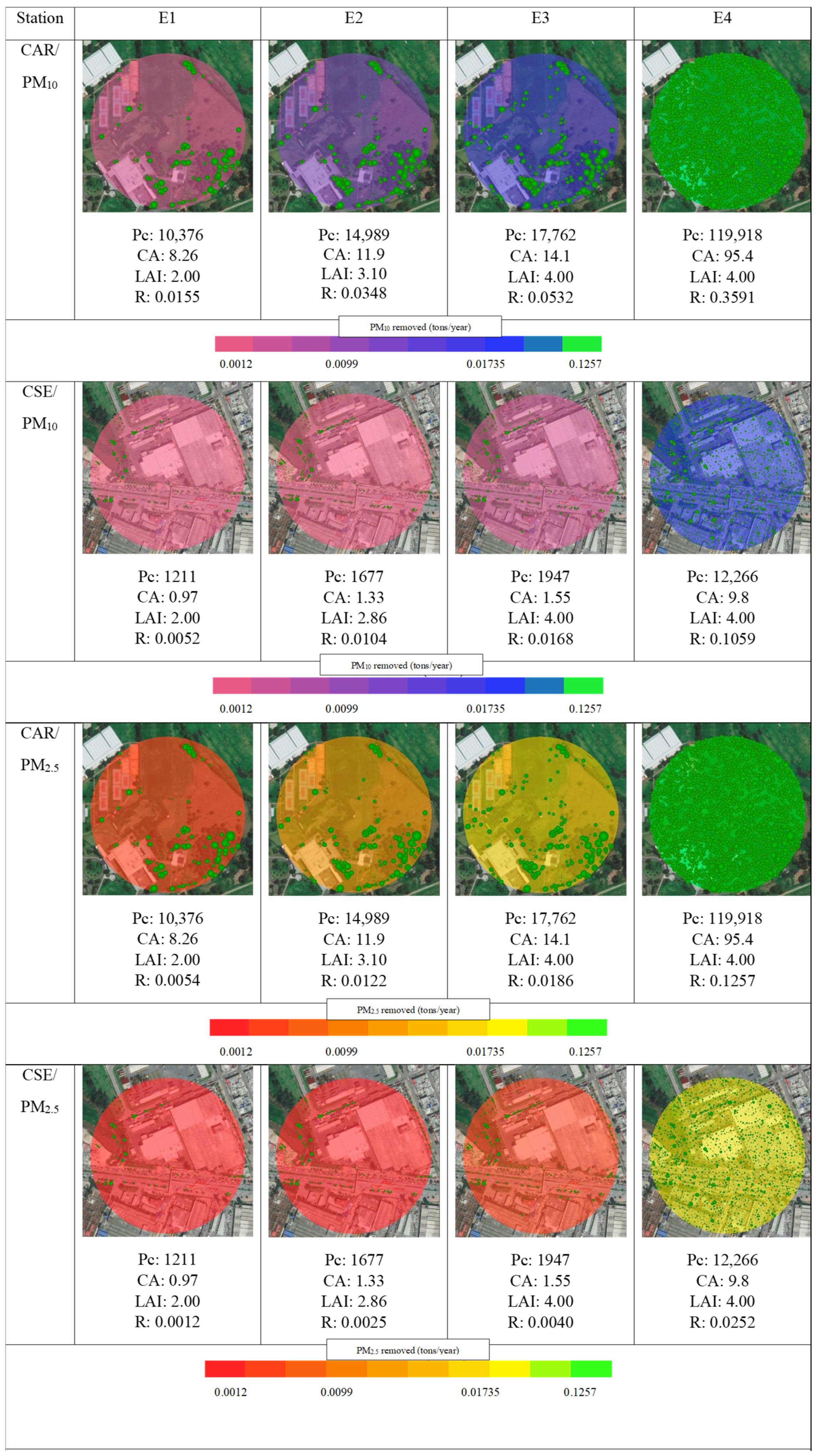
3.2. PM Removal Simulation Scenarios

During the simulations of the four study scenarios, special attention was given to the CAR and CSE monitoring stations, as these stations recorded the highest (CA = 65.9%) and lowest (CA = 16.5%) tree cover during the reference scenario. This E2 scenario (Table 2) was used as a reference to compare its results with the other study scenarios (E1, E3, and E4). The results showed that for all simulated scenarios, there was a maximum and minimum PM₁₀ removal of 0.359 and 0.005 tons/year, respectively. For PM_2.5, the maximum and minimum removals were 0.700 and 0.005 tons/year, respectively. The scenarios that showed the highest and lowest PM₁₀ removal were those associated with the highest (E4) and lowest (E1) CAs and LAIs, respectively (

Table 4. Scenario simulation results for PM₁₀ at CAR and CSE monitoring stations.

CAR
	E1: Decline (–)			E2: Reference			E3: Increase (+)			E4: Brooklyn
CA (%)	8.26			11.9			14.1			95.4
CA (m2)	10,376			14,990			17,762			119,918
Percentage of annual improvement—air quality (I)	0.0957			0.138			0.164			1.091
PM removal (tons/year)	0.0241			0.0348			0.0412			0.2783
Percentage of improvement vs. E2 (%)	−30.8			-			18.5			700.0
	E1	E1 (Q1)	E1 (Q3)	E1	E1 (Q1)	E1 (Q3)	E1	E1 (Q1)	E1 (Q3)	E1	E1 (Q1)	E1 (Q3)
IAF (m2/m2)	3.10	2.00	4.00	3.10	2.00	4.00	3.10	2.00	4.00	3.10	2.00	4.00
Percentage of annual improvement—air quality (I)	0.0957	0.0618	0.123	0.138	0.0892	0.178	0.164	0.106	0.211	1.091	0.708	1.402
PM removal (tons/year)	0.0241	0.0155	0.0311	0.0348	0.0224	0.0449	0.0412	0.0266	0.0532	0.2783	0.1795	0.3591
PM removal (ton/[Ha × year])	0.0019	0.0012	0.0025	0.0028	0.0018	0.0036	0.0033	0.0021	0.0042	0.0221	0.0143	0.0286
Percentage of improvement vs. E2 (%)	−30.8	−55.3	−10.68		−35.5	29.03	18.5	−23.6	52.90	700.00	416.13	932.26
CSE
	E1: Decline (–)			E2: Reference			E3: Increase (+)			E4: Brooklyn
CA (%)	0.964			1.33			1.55			9.8
CA (m2)	1211			1677			1947			12,266
Percentage of annual improvement—air quality (I)	0.0103			0.014			0.017			0.105
PM removal (tons/year)	0.0075			0.0104			0.0120			0.0757
Percentage of improvement vs. E2 (%)	−27.8			-			16.1			631.4
	E1	E1 (Q1)	E1 (Q3)	E1	E1 (Q1)	E1 (Q3)	E1	E1 (Q1)	E1 (Q3)	E1	E1 (Q1)	E1 (Q3)
IAF (m2/m2)	2.86	2.00	4.00	2.86	2.00	4.00	2.86	2.00	4.00	2.86	2.00	4.00
Percentage of annual improvement—air quality (I)	0.0103	0.0072	0.014	0.014	0.0100	0.020	0.017	0.012	0.023	0.105	0.073	0.146
PM removal (tons/year)	0.0075	0.0052	0.0105	0.0104	0.0072	0.0145	0.0120	0.0084	0.0168	0.0757	0.0530	0.1059
PM removal (ton/[Ha × year])	0.0006	0.0004	0.0008	0.0008	0.0006	0.0012	0.0010	0.0007	0.0013	0.0060	0.0042	0.0084
Percentage of improvement vs. E2 (%)	−27.8	−49.5	1.04		−30.1	39.86	16.1	−18.8	62.40	631.45	411.50	923.00

).

Under the decreased CA scenario (E1, Table 4), PM₁₀ removal (tons/year) decreased by 30.8% at CAR (CA: 8.30%) and 27.9% at CSE (CA: 1.0%) compared to the reference scenario (E2), where CA was 11.9% and 1.30%, respectively. At CAR, a 3.64% CA reduction resulted in a 30.8% decrease in annual PM₁₀ removal. At CSE, a 0.37% CA reduction led to a 27.9% decrease in PM₁₀ removal. Despite the CA reduction at CAR being 9.84 times greater than at CSE, the difference in PM₁₀ removal decrease was only 2.90% (Figure 5). Average hourly PM₁₀ concentrations were 21.6 μg/m³ at CAR and 63.6 μg/m³ at CSE. Similarly, annual PM_2.5 removal capacity decreased by 31.2% at CAR (CA: 8.30%) and 28% at CSE (CA: 1.0%) compared to the E2 scenario (CAR CA: 11.9%; CSE CA: 1.30%). At CAR, a 3.64% CA reduction resulted in a 31.2% decrease in annual PM_2.5 removal. At CSE, a 0.37% CA decrease led to a 28% reduction in annual PM_2.5 removal (

Table 5. Scenario simulation results for PM_2.5 at CAR and CSE monitoring stations.

CAR
	E1: Decline (–)			E2: Reference			E3: Increase (+)			E4: Brooklyn
CA (%)	8.26			11.9			14.1			95.4
CA (%)	10,376			14,990			17,762			119,918
CA (m2)	0.0473			0.068			0.081			0.542
Percentage of annual improvement—air quality (I)	0.0084			0.0122			0.0144			0.0973
PM removal (tons/year)	−30.8			-			18.5			700.0
Percentage of improvement vs. E2 (%)	E1	E1 (Q1)	E1 (Q3)	E1	E1 (Q1)	E1 (Q3)	E1	E1 (Q1)	E1 (Q3)	E1	E1 (Q1)	E1 (Q3)
	3.10	2.00	4.00	3.10	2.00	4.00	3.10	2.00	4.00	3.10	2.00	4.00
IAF (m2/m2)	0.0473	0.0302	0.061	0.068	0.0436	0.088	0.081	0.052	0.105	0.542	0.347	0.700
Percentage of annual improvement—air quality (I)	0.0084	0.0054	0.0109	0.0122	0.0078	0.0157	0.0144	0.0092	0.0186	0.0973	0.0620	0.1257
PM removal (tons/year)	0.0007	0.0004	0.0009	0.0010	0.0006	0.0013	0.0011	0.0007	0.0015	0.0077	0.0049	0.0100
PM removal (ton/[Ha × year])	−30.8	−55.8	−10.50		−36.2	29.29	18.5	−24.4	53.20	700.00	410.30	934.30
CSE
	E1: Decline (–)			E2: Reference			E3: Increase (+)			E4: Brooklyn
CA (%)	0.96			1.33			1.5			9.8
CA (m2)	1211			1677			1947			12,266
Percentage of annual improvement—air quality (I)	0.0044			0.006			0.007			0.045
PM removal (tons/year)	0.0018			0.0025			0.0029			0.0180
Percentage of improvement vs. E2 (%)	−27.8			-			16.1			631.4
	E1	E1 (Q1)	E1 (Q3)	E1	E1 (Q1)	E1 (Q3)	E1	E1 (Q1)	E1 (Q3)	E1	E1 (Q1)	E1 (Q3)
IAF (m2/m2)	2.86	2.00	4.00	2.86	2.00	4.00	2.86	2.00	4.00	2.86	2.00	4.00
Percentage of annual improvement—air quality (I)	0.0044	0.0030	0.006	0.006	0.0042	0.008	0.007	0.005	0.010	0.045	0.031	0.063
PM removal (tons/year)	0.0018	0.0012	0.0025	0.0025	0.0017	0.0034	0.0029	0.0020	0.0040	0.0180	0.0125	0.0252
PM removal (ton/[Ha × year])	0.0001	0.0001	0.0002	0.0002	0.0001	0.0003	0.0002	0.0002	0.0003	0.0014	0.0010	0.0020
Percentage of improvement vs. E2 (%)	−27.8	−49.7	1.32		−30.4	40.25	16.1	−19.2	62.85	631.45	409.13	925.87

). Despite the CA reduction at CAR being 9.84 times greater than at CSE, the difference in PM_2.5 removal decrease was only 3.2%. Average hourly PM_2.5 concentrations were 14 μg/m³ at CAR and 29.2 μg/m³ at CSE.

Regarding the scenario of increased CA (E3, Table 4), the results showed an increase in annual PM₁₀ removal of 15.5% and 13.3% at the CAR (CA: 14.1%) and CSE (CA: 1.60%) stations, respectively. This was compared to the E2 scenario, where CA represented 11.9% and 1.30% of the study area, respectively. At the CAR station, a 2.20% increase in CA resulted in a 15.5% increase in annual PM₁₀ removal. At the CSE station, a 0.22% increase in CA resulted in a 13.3% increase in PM₁₀ removal (Figure 5). Although the increase in CA at the CAR station was 10 times greater than at the CSE station, the difference in the increase in PM₁₀ removal was only 2.20% (CAR/PM₁₀: 21.6 µg/m³ and CSE/PM₁₀: 63.6 µg/m³). Similarly, the results obtained for the E3 scenario revealed an increase in annual PM_2.5 removal capacity of 15.3% at the CAR station (CA: 14.1%) and 13.8% at the CSE station (CA: 1.60%). These increases were compared to the E2 scenario, where CA reached 11.9% and 1.30% at the CAR and CSE stations, respectively. At the CAR station, a 2.20% increase in CA translated to a 15.3% increase in annual PM_2.5 removals. At the CSE station, a 0.17% increase in CA resulted in a 13.8% increase in annual PM_2.5 removals (Table 5). Although the increase in CA at the CAR station was 10 times greater than at the CSE station, the difference in the increase in PM_2.5 removals was only 1.50% (CAR/PM_2.5: 14 µg/m³ and CSE/PM_2.5: 29.2 µg/m³).

Regarding the Brooklyn scenario (E4, Table 4), which involved increasing CA eightfold and with a maximum LAI (4 m²/m²), the results showed a significant increase in annual PM₁₀ removal of 700% and 630% at the CAR (CA: 95.4%) and CSE (CA: 9.80%) stations, respectively. This was compared to the E2 scenario (CA, CAR: 11.9% and CSE: 1.30%). At the CAR station, an 81.3% increase in CA resulted in a 700% increase in annual PM₁₀ removal. At the CSE station, an 8.25% increase in CA resulted in a 628% increase in PM₁₀ removal (Figure 5). Although the increase in CA at the CAR station was 9.73 times greater than at the CSE station, the difference in the increase in annual PM₁₀ removal was 70%. Likewise, the results obtained for E4 showed an increase in annual PM_2.5 removal capacity of 698% at the CAR station (CA: 95.4%) and 620% at the CSE station (CA: 9.80%). These increases were compared to E2, where CA reached 11.9% and 1.30% at the CAR and CSE stations, respectively. These results confirmed that the significant increase in CA significantly impacted annual PM_2.5 removals, improving urban air quality. At the CAR station, an 81.3% increase in CA translated to a 698% increase in annual PM_2.5 removals. At the CSE station, an 8.3% increase in CA resulted in a 620% increase in annual PM_2.5 removals (Table 5). Although the increase in CA at the CAR station was 9.73 times greater than at the CSE station, the difference in the increase in annual PM_2.5 removals was 78%.

In this study, multivariate regression models (R² > 0.90) were developed as a simplified, rapid application method to determine PM removal and the percentage improvement in air quality based on CA and LAI (

Table 6. Multiple linear regression models between CA and LAI versus PM removal and percent improvement in air quality at CSE and CAR monitoring stations.

Variable	Station/Air Pollutant
	CAR/PM10	R2	CSE/PM10	R2
Average improvement—I (%)	I = −0.13 + (0.011 × CA) + (0.043 × LAI)	0.912	I = −0.016 + (0.013 × CA) + (0.005 × LAI)	0.909
Removal—R (tons/year)	R = −0.033 + (0.003 × CA) + (0.011 × LAI)	0.912	R = −0.012 + (0.009 × CA) + (0.003 × LAI)	0.908
	CAR/PM2.5	R2	CSE/PM2.5	R2
Average improvement—I (%)	I = −0.065 + (0.006 × CA) + (0.021 × LAI)	0.911	I = −0.006 + (0.005 × CA) + (0.002 × LAI)	0.923
Removal—R (tons/year)	R = −0.012 + (0.001 × CA) + (0.004 × LAI)	0.911	R = −0.002 + (0.002 × CA) + (0.001 × LAI)	0.923

Note. CA: Tree cover (%), LAI: Leaf Area Index (m²/m²), R: PM removal (tons/year), and I: Percentage improvement in air quality (%).

). The results showed that a significant increase in CA and LAI led to greater PM removal, although percentage improvements in air quality were modest, generally below 2%, even under the E4 scenario. For example, at the CAR station, an extreme (hypothetical) scenario with 100% CA and a maximum LAI of 6 m²/m² resulted in PM₁₀ removals of 0.333 tons/year and PM_2.5 removals of 0.112 tons/year. At the CSE station, this extreme scenario resulted in PM₁₀ removals of 0.906 tons/year and PM_2.5 removals of 0.204 tons/year. These results corresponded to an urban circular area with an influence radius of 200 m. Extrapolation to larger urban areas indicated significant removal potential for the studied megacity. However, a linear relationship between CA and PM removal might not be entirely accurate, with urban configuration and impervious surfaces also being important factors.

4. Discussion

4.1. PM Removal Model

The strong positive correlation between urban CA and PM₁₀ removal (R² = 0.987) across monitoring stations (E2 scenario, Table 2) reinforces the critical role of urban vegetation in mitigating PM pollution [61,62]. Higher annual PM₁₀ removal at CAR and MIN stations, with greater CA, underscores the capacity of substantial tree cover to enhance urban air quality. Conversely, lower PM₁₀ removal at the CSE station, with significantly lower CA, aligns with findings that PM₁₀ removal efficiency is linked to urban forest biomass density and distribution [15]. The notable finding that PM₁₀ removal at CSE was lower than at CAR and MIN, despite higher PM₁₀ concentrations, suggests that tree cover extent is more crucial for PM₁₀ removal than ambient concentration. This highlights the necessity of sufficient vegetation for significant pollutant removal. The average annual air quality improvement of 1.05 ± 0.01% per percentage unit of CA provides a valuable metric for assessing urban trees’ impact on PM₁₀ reduction, informing urban planning and management strategies.

The consistent trend of higher annual PM_2.5 removal at the CAR and MIN stations, mirroring PM₁₀ findings and correlating with their greater CA (Figure 3), substantiates the role of urban tree cover in mitigating fine PM. The significantly higher average CA at CAR and MIN compared to other stations directly translated to improved PM_2.5 air quality, as evidenced by their higher improvement percentages. The strong correlation between annual PM_2.5 removal and CA (R² = 0.918) reinforces the positive impact of urban trees on reducing this critical air pollutant. The KEN station provides crucial insight into PM_2.5 removal dynamics. Despite high PM_2.5 concentrations, the relatively modest removal suggests that factors beyond concentration, such as tree species characteristics and leaf area, play a significant role. The substantial reduction in PM_2.5 removal at KEN following decreased ambient PM_2.5 concentrations during the COVID-19 pandemic indicates that pollutant availability is a limiting factor for removal efficiency, supported by prior research [63]. This observation underscores that while urban trees offer valuable air purification, their removal capacity is linked to atmospheric conditions. The average air quality improvement of 0.039 ± 0.005% for PM_2.5 across all stations highlights the overall contribution of the existing urban forest in mitigating fine PM pollution.

The observed difference in annual air quality improvement per percentage unit of CA, with PM₁₀ showing a 32.1% higher improvement than PM_2.5 (0.71 ± 0.09%), can be attributed to the inclusion of PM_2.5 resuspension in the modeling, which was not a factor in PM₁₀ simulations. This methodological distinction led to lower PM_2.5 removal estimates and consequently, lower air quality improvement. Higher annual air quality improvements per percentage unit of CA for PM_2.5 at KEN and CSE stations, despite lower overall CA, reflect the influence of higher PM_2.5 concentrations at these locations. This aligns with the understanding that air quality improvements from tree cover are influenced by both vegetation extent and ambient pollutant concentrations [64]. Given stable precipitation and wind speed conditions across monitoring stations, it is reasonable to infer consistent mixing layer heights, suggesting CA and PM concentrations were primary drivers influencing UFORE-D modeling outcomes. Furthermore, PM deposition rate is influenced by tree species-specific traits, such as leaf morphology [15,65], contributing to variations in removal efficiency. The finding that average annual air quality improvement per percentage unit of CA is generally 1.0% or less [66,67] supports the notion that while the impact per unit of tree cover might seem modest, a substantial and well-distributed urban forest can collectively provide significant long-term benefits in mitigating urban PM pollution.

The sensitivity analysis, using the graphical method suggested by Hirabayashi et al. [29], effectively evaluated the model’s logic and applicability across the four simulated tree cover scenarios (Table 2). Using PM₁₀ concentration and LAI as input variables, as well as total PM₁₀ removal and annual air quality improvement as outputs, allowed for a robust assessment. The selection of 2014 PM₁₀ data from the CAR station, with its high CA, provided a relevant case for verifying the model’s behavior. The predictable air quality improvement values generated by the PM₁₀ modeling, which aligned with findings from other studies [29,34,68,69], including the average 1% improvement reported by Nowak et al. [62] in U.S. cities, bolsters confidence in the model’s reliability. The sensitivity analysis demonstrated that increasing CA positively correlated with air quality improvement, and that wind speed acted as a modulating factor, with simulated improvements increasing significantly (up to tenfold) under maximum wind speed conditions. The regression model coefficients highlighted the substantial influence of both CA (0.609β) and LAI (0.774β) on annual air quality improvement, with LAI emerging as a more influential factor than the sheer number of trees (CA). This suggests that the structural characteristics of the urban forest canopy play a more critical role in PM₁₀ removal than just the extent of coverage. The consistent results obtained from the sensitivity analysis for PM_2.5 concentrations further validate the overall robustness and applicability of the modeling approach used in this study.

The model’s validity was further established through a comparison of its results with those from existing literature under the reference scenario (E2, Table 2) across all monitoring stations. The simulations indicated lower PM₁₀ (0.010 tons/year) and PM_2.5 (0.0025 tons/year) removal at the CSE station, which had the lowest CA (0.168 Ha). Conversely, the CAR station, with the highest CA (1.49 Ha), showed higher removal rates of 0.035 tons/year for PM₁₀ and 0.012 tons/year for PM_2.5. These findings align with the trends reported by Jayasooriya et al. [60], who observed that an approximate eightfold increase in CA led to a sixfold increase in PM removal (from 0.007 to 0.043 tons/year). Notably, despite exhibiting the lowest absolute PM removal, the CSE and KEN stations demonstrated high PM removal potential per hectare (Table 3). This observation supports the assertion by Arroyave et al. [67] that ambient PM concentration is a key driver of removal, as higher concentrations provide a greater pool of pollutants for capture by urban trees.

The observed homogeneity in simulated PM removal values across the monitoring stations, likely stemming from their similar climatic, morphological, and topographic characteristics, lends further credibility to the model’s outputs. The PM₁₀ removal rates simulated for CAR, MIN, and SCR (0.020–0.023 tons/[Ha × year]) closely mirrored the 0.0254 tons/(Ha × year) reported for Beijing (China) using the UFORE model [70], suggesting a consistent order of magnitude in PM₁₀ removal by urban trees across different urban environments. Similarly, the simulated PM₁₀ removal for the USQ station (0.018 tons/[Ha × year]) was in line with the findings from studies conducted in Italy [71,72], indicating a degree of transferability in the model’s estimations. For PM_2.5, the simulated removal at the CSE monitoring station (0.0147 tons/[Ha × year]) was comparable to the 0.0160 tons/(Ha × year) reported in Shenzhen (China) using the I-Tree software V.6 [73]. Furthermore, the PM_2.5 removal rates simulated for CAR, KEN, MIN, SCR, and USQ (0.0066–0.0097 tons/[Ha × year]) were of a similar magnitude to the 0.0715 tons/(Ha × year) reported in Medellín (Colombia) using the same software [67], although the latter value is somewhat higher, potentially reflecting differences in urban forest structure or local PM_2.5 characteristics. Overall, the consistency of our simulation results with findings from diverse geographical locations and using different modeling approaches strengthens the confidence in the validity and applicability of the model developed in this study for assessing the role of urban trees in PM removal.

4.2. PM Removal Simulation Scenarios

The results of this study evidenced for E1 a clear correlation between the decrease in CA and the reduction in annual PM removal capacity in urban environments, reinforcing the importance of trees in improving air quality. For both PM₁₀ and PM_2.5, a decrease in annual removal was observed when CA was reduced, with similar reduction percentages for both types of particles at the CAR and CSE stations, suggesting a consistent response of the tree system and the UFORE-D modeling performed. However, the magnitude of the reduction was more pronounced at the CSE station, which had higher ambient concentrations of both types of particles, indicating that removal efficiency increased in more polluted environments (Figure 5). Despite slight differences in reduction percentages between PM₁₀ and PM_2.5, the similarity in trends suggested that the decrease in CA proportionally affected the removal of both PM fractions. The discrepancy between the large difference in CA reduction and the small difference in PM removal reduction highlighted the complexity of interactions between trees and air quality, suggesting that once a minimum CA threshold was exceeded, ambient concentrations had a greater impact on removal than the number of tree individuals. These findings also underscored the need to preserve and expand CA in urban areas, especially in zones with high PM concentrations. The E1 scenario was a realistic scenario, as it was simulated according to the average tree felling in the megacity under study, based on historical data presented in the Bogotá Environmental Observatory tree inventory [59]. Indeed, it was recommended to maintain CA, as tree felling implied a decrease in annual PM removal at the monitoring stations under study.

The comparative analysis between PM₁₀ and PM_2.5 for E3 revealed that the increase in CA significantly increased the removal of both PM fractions, corroborating the vital role of urban trees in improving air quality. This simulation scenario considered the average increase in tree individuals planted in the megacity, based on historical data reported in the Bogotá Environmental Observatory tree inventory [59]. Increases in annual PM₁₀ removal of 15.5% and 13.3% were observed at the CAR and CSE stations, while for PM_2.5, the increases were 15.3% and 13.8%, respectively. Although the increase in CA at CAR was 10 times greater than at CSE, the difference in the increase in removal was only 2.20% for PM₁₀ and 1.50% for PM_2.5 (Figure 5). This discrepancy was attributed to differences in ambient concentrations, being higher at CSE (PM₁₀: 63.6 µg/m³ and PM_2.5: 29.2 µg/m³) than at CAR (PM₁₀: 21.6 µg/m³ and PM_2.5: 14 µg/m³). These results suggested that removal efficiency was enhanced by high PM concentrations and that beyond a CA threshold, ambient concentrations exerted a greater influence on PM removal. Yang et al. [68] obtained similar results. Although the trends were similar for both PM fractions, slight variations in the magnitude of the removal increase were observed, possibly due to differences in the physical properties of the particles [71]. These findings also highlighted the importance of increasing CA, especially in areas with high PM concentrations, considering additional factors such as tree species and meteorological conditions [72,73].

The results of this study demonstrated that an extreme increase in CA (E4) significantly increased PM removal, improving urban air quality. This E4 scenario increased CA by 80% compared to the E2 scenario, regardless of the availability of area for planting tree individuals at each of the two monitoring stations considered. For both PM₁₀ and PM_2.5, a similar percentage increase in annual removal was observed when CA was increased, suggesting a positive and comparable effect of urban trees on both PM fractions (Figure 5). However, differences in hourly PM₁₀ and PM_2.5 concentrations between the monitoring stations (CAR and CSE) possibly influenced the magnitude of the removal increase. Although the increase in CA was much greater at CAR, the difference in the increase in removal was not proportionally as large, suggesting that the higher concentration at CSE may have enhanced the effect of CA. These findings were consistent with previous studies [74], highlighting the capacity of urban trees to improve air quality by removing PM. However, the efficiency of this removal could vary depending on the tree species, foliage density, and meteorological conditions [72,75]. In practice, this E4 scenario could not be implemented at the CAR and CSE stations due to the limited area available for planting tree individuals.

As observed in Figure 5 (E4), the simulated CA area overlapped with impervious cover and bare soil at the CAR and CSE monitoring stations. This generated the need to possibly consider other types of green infrastructure to achieve the total simulated CA area for E4. Although this analysis was beyond the scope of this study, the findings suggested that implementing green roofs and walls could be an option for removing urban PM. Jayasooriya et al. [60] evaluated, through various scenarios, the configuration of other infrastructures such as green roofs and walls, and identified which trees provided the greatest PM removal capacity. These researchers reported that implementing green roofs and walls provided significant benefits in urban areas where there was limited availability of areas for planting trees. Other studies reported that PM removal by green infrastructure varied according to pollutant emissions, distance between the source and green infrastructure, and the percentage of area covered by green infrastructure and its type [76]. Moreover, it was reported that green infrastructure could be a beneficial passive method, as it not only removed PM but also reduced the urban heat island effect, controlled surface runoff, and influenced the recreational activities, health, and well-being of residents [65,77]. However, when planting urban trees, a configuration that enhances the canyon effect should be avoided. That is, when tree canopies close, air flow turbulence decreases below the canopies, leading to high concentrations of pollutants [20,77].

The CSE station, with a larger impervious area, showed lower annual PM removals in all scenarios considered, despite having higher PM concentrations. This underscored the importance of considering urban heterogeneity when modeling pollutant removal. This extreme scenario (CA: 100%, LAI: 6 m²/m²) showed relative improvements close to 700% in PM₁₀ and PM_2.5 removals, indicating that while the percentage increase in PM removal could be high, the absolute reduction in pollutants was limited (<1.0%). For example, at the CAR station, and under this extreme scenario (CA: 100% and LAI: 6 m²/m²), an annual air quality improvement of 1.23% for PM₁₀ and 0.66% for PM_2.5 was simulated. At the CSE station, this extreme scenario resulted in an annual air quality improvement of 1.31% for PM₁₀ and 0.51% for PM_2.5 (Table 6). Extrapolating this extreme scenario to the entire megacity under study resulted in a potential removal of 879 tons/year of PM₁₀ and 476 tons/year of PM_2.5. Although these values represented a significant contribution to the reduction of PM₁₀ and PM_2.5 pollution, they were comparatively low relative to the megacity’s total emissions (57,577 tons/year of PM₁₀, for 2018). Lastly, modeling PM removal by urban trees was complex and influenced by multiple factors. Future studies should consider including variables such as urban geometric configuration, the presence of green infrastructure (green roofs and walls), and variability in tree species. Moreover, it is recommended to use models that cover larger areas to obtain more accurate estimates at the megacity level. Indeed, the implementation of urban tree strategies should be accompanied by other emission control measures to achieve significant improvements in urban air quality.

5. Conclusions

The results of this study on the influence of urban trees on PM₁₀ and PM_2.5 concentrations in a high-altitude Latin American megacity using UFORE-D modeling allow the following conclusions to be drawn.

The model shows a strong positive correlation between CA and PM removal, reinforcing the critical role of urban forests in improving air quality. PM removal is influenced by both CA and ambient pollutant concentrations, with higher concentrations generating higher removal rates, although CA remains a more significant factor. The model’s sensitivity analysis confirms that increasing CA, represented by the LAI, significantly enhances air quality improvement, particularly under higher wind speeds. The annual air quality improvement per percentage unit of CA is greater for PM₁₀ than for PM_2.5, which could be attributed to the inclusion of resuspension in PM_2.5 modeling. These findings highlight the model’s applicability in evaluating the benefits of urban trees in mitigating PM pollution, providing valuable information for urban planning and air quality management. This study also underscores the importance of strategically increasing CA to maximize PM removal, advocating for the integration of urban forestry into comprehensive air pollution mitigation strategies.

The magnitude of PM removal is significantly influenced by ambient pollutant concentrations, with higher concentrations enhancing removal efficiency in all simulated scenarios. The analysis highlights that while increasing CA consistently improves PM removal, the proportional impact varies, with diminishing returns observed beyond a certain threshold. The extreme E4 scenario, although theoretically impactful, underscores practical limitations in achieving substantial CA increases due to urban spatial constraints. This necessitates exploring integrated green infrastructure solutions, such as green roofs and walls, to complement urban forestry efforts. Moreover, the study emphasizes the complex interaction between CA, LAI, and urban configuration in PM removal. Despite significant percentage improvements in PM removal under extreme CA scenarios, the absolute reduction of pollutants remains limited, requiring a holistic approach that integrates urban forestry with rigorous emission control strategies.

Finally, the following limitations were part of this study. The models used did not include localized meteorological variations and urban geometric factors. To optimize the accuracy and applicability of the models, future research should focus on incorporating these variables. In future studies, it would also be relevant to perform a comparative analysis between this high-altitude megacity and other urban areas with different conditions, in order to identify possible differences in the simulation of the PM retention capacity of urban trees. Moreover, it is crucial to explore species-specific removal efficiencies to develop more precise and contextualized air quality management strategies. Integrating these factors will enable a more comprehensive and realistic assessment of the impact of urban trees, facilitating the implementation of effective measures to mitigate atmospheric pollution.

References

1. Ren, Z.; Liu, X.; Liu, T.; Chen, D.; Jiao, K.; Wang, X.; Suo, J.; Yang, H.; Liao, J.; Ma, L. Effect of Ambient Fine Particulates (PM2.5) on Hospital Admissions for Respiratory and Cardiovascular Diseases in Wuhan, China. Respir. Res. 2021, 22, 128. [Google Scholar] [CrossRef] [PubMed]
2. Dastoorpoor, M.; Riahi, A.; Yazdaninejhad, H.; Borsi, S.H.; Khanjani, N.; Khodadadi, N.; Mohammadi, M.J.; Aghababaeian, H. Exposure to Particulate Matter and Carbon Monoxide and Cause-Specific Cardiovascular-Respiratory Disease Mortality in Ahvaz. Toxin Rev. 2021, 40, 1362–1372. [Google Scholar] [CrossRef]
3. Gryech, I.; Ghogho, M.; Mahraoui, C.; Kobbane, A. An Exploration of Features Impacting Respiratory Diseases in Urban Areas. Int. J. Environ. Res. Public Health 2022, 19, 3095. [Google Scholar] [CrossRef]
4. Ochoa-Alvarado, L.M.; Zafra-Mejía, C.A.; Rondón-Quintana, H.A. Multitemporal Analysis of the Influence of PM10 on Human Mortality According to Urban Land Cover. Atmosphere 2022, 13, 1949. [Google Scholar] [CrossRef]
5. Zhang, L.; Wilson, J.P.; Zhao, N.; Zhang, W.; Wu, Y. The Dynamics of Cardiovascular and Respiratory Deaths Attributed to Long-Term PM2.5 Exposures in Global Megacities. Sci. Total Environ. 2022, 842, 156951. [Google Scholar] [CrossRef]
6. Bhunia, G.S.; Ghosh, A.; Shit, P.K. Comprehensive Spatio-Temporal Analysis of Ambient Air Quality of Kolkata Municipal Corporation, Kolkata (West Bengal, India) during 2017–2020. Arab. J. Geosci. 2022, 15, 1782. [Google Scholar] [CrossRef]
7. Chen, L.; Zhang, J.; Huang, X.; Li, H.; Dong, G.; Wei, S. Characteristics and Pollution Formation Mechanism of Atmospheric Fine Particles in the Megacity of Chengdu, China. Atmos. Res. 2022, 273, 106172. [Google Scholar] [CrossRef]
8. Wu, C.; Wang, H.; Cai, W.; He, H.; Ni, A.; Peng, Z. Impact of the COVID-19 Lockdown on Roadside Traffic-Related Air Pollution in Shanghai, China. Build. Environ. 2021, 194, 107718. [Google Scholar] [CrossRef]
9. Pai, S.J.; Carter, T.S.; Heald, C.L.; Kroll, J.H. Updated World Health Organization Air Quality Guidelines Highlight the Importance of Non-Anthropogenic PM2.5. Environ. Sci. Technol. Lett. 2022, 9, 501–506. [Google Scholar] [CrossRef]
10. Kim, M.-J.; Chang, Y.-S.; Kim, S.-M. Impact of Income, Density, and Population Size on PM2.5 Pollutions: A Scaling Analysis of 254 Large Cities in Six Developed Countries. Int. J. Environ. Res. Public Health 2021, 18, 9019. [Google Scholar] [CrossRef]
11. Han, C.; Xu, R.; Ye, T.; Xie, Y.; Zhao, Y.; Liu, H.; Yu, W.; Zhang, Y.; Li, S.; Zhang, Z.; et al. Mortality Burden Due to Long-Term Exposure to Ambient PM2.5 above the New WHO Air Quality Guideline Based on 296 Cities in China. Environ. Int. 2022, 166, 107331. [Google Scholar] [CrossRef] [PubMed]
12. Li, X.; Zhang, T.; Sun, F.; Song, X.; Zhang, Y.; Huang, F.; Yuan, C.; Yu, H.; Zhang, G.; Qi, F.; et al. The Relationship between Particulate Matter Retention Capacity and Leaf Surface Micromorphology of Ten Tree Species in Hangzhou, China. Sci. Total Environ. 2021, 771, 144812. [Google Scholar] [CrossRef] [PubMed]
13. Singh, A.K.; Kumar, M.; Bauddh, K.; Singh, A.; Singh, P.; Madhav, S.; Shukla, S.K. Environmental Impacts of Air Pollution and Its Abatement by Plant Species: A Comprehensive Review. Environ. Sci. Pollut. Res. 2023, 30, 79587–79616. [Google Scholar] [CrossRef] [PubMed]
14. Chen, D.; Yin, S.; Zhang, X.; Lyu, J.; Zhang, Y.; Zhu, Y.; Yan, J. A High-Resolution Study of PM2.5 Accumulation inside Leaves in Leaf Stomata Compared with Non-Stomatal Areas Using Three-Dimensional X-Ray Microscopy. Sci. Total Environ. 2022, 852, 158543. [Google Scholar] [CrossRef]
15. Rodríguez-Santamaría, K.; Zafra-Mejía, C.A.; Rondón-Quintana, H.A. Macro-Morphological Traits of Leaves for Urban Tree Selection for Air Pollution Biomonitoring: A Review. Biosensors 2022, 12, 812. [Google Scholar] [CrossRef]
16. Ossola, R.; Farmer, D. The Chemical Landscape of Leaf Surfaces and Its Interaction with the Atmosphere. Chem. Rev. 2024, 124, 5764–5794. [Google Scholar] [CrossRef]
17. Xue, W.; Lin, Y.; Sun, Z.; Long, Y.; Chen, D.; Yin, S. Effects of Leaf Trait Variability on PM Retention: A Systematic Review. Atmosphere 2025, 16, 170. [Google Scholar] [CrossRef]
18. Zafra-Mejía, C.; Suárez-López, J.; Rondón-Quintana, H. Analysis of Particulate Matter Concentration Intercepted by Trees of a Latin-American Megacity. Forests 2021, 12, 723. [Google Scholar] [CrossRef]
19. Maison, A.; Lugon, L.; Park, S.-J.; Boissard, C.; Faucheux, A.; Gros, V.; Kalalian, C.; Kim, Y.; Leymarie, J.; Petit, J.-E.; et al. Contrasting Effects of Urban Trees on Air Quality: From the Aerodynamic Effects in Streets to Impacts of Biogenic Emissions in Cities. Sci. Total Environ. 2024, 946, 174116. [Google Scholar] [CrossRef]
20. McDonald, A.G.; Bealey, W.J.; Fowler, D.; Dragosits, U.; Skiba, U.; Smith, R.I.; Donovan, R.G.; Brett, H.E.; Hewitt, C.N.; Nemitz, E. Quantifying the Effect of Urban Tree Planting on Concentrations and Depositions of PM10 in Two UK Conurbations. Atmos. Environ. 2007, 41, 8455–8467. [Google Scholar] [CrossRef]
21. Kroeger, T.; McDonald, R.I.; Boucher, T.; Zhang, P.; Wang, L. Where the People Are: Current Trends and Future Potential Targeted Investments in Urban Trees for PM10 and Temperature Mitigation in 27 U.S. Cities. Landsc. Urban Plan. 2018, 177, 227–240. [Google Scholar] [CrossRef]
22. Pachón, J.E.; Galvis, B.; Lombana, O.; Carmona, L.G.; Fajardo, S.; Rincón, A.; Meneses, S.; Chaparro, R.; Nedbor-Gross, R.; Henderson, B. Development and Evaluation of a Comprehensive Atmospheric Emission Inventory for Air Quality Modeling in the Megacity of Bogotá. Atmosphere 2018, 9, 49. [Google Scholar] [CrossRef]
23. Blanco-Becerra, L.C.; Gáfaro-Rojas, A.I.; Rojas-Roa, N.Y. Influence of Precipitation Scavenging on the PM2.5/PM10 Ratio at the Kennedy Locality of Bogota, Colombia. Rev. Fac. Ing. Univ. Antioq. 2015, 76, 58–65. [Google Scholar] [CrossRef]
24. Kumar, A.; Jiménez, R.; Belalcázar, L.C.; Rojas, N.Y. Application of WRF-Chem Model to Simulate PM10 Concentration over Bogota. Aerosol Air Qual. Res. 2016, 16, 1206–1221. [Google Scholar] [CrossRef]
25. Jin, Z.; Velásquez Angel, M.A.; Mura, I.; Franco, J.F. Enriched Spatial Analysis of Air Pollution: Application to the City of Bogotá, Colombia. Front. Environ. Sci. 2022, 10, 966560. [Google Scholar] [CrossRef]
26. Vos, P.E.J.; Maiheu, B.; Vankerkom, J.; Janssen, S. Improving Local Air Quality in Cities: To Tree or Not to Tree? Environ. Pollut. 2013, 183, 113–122. [Google Scholar] [CrossRef]
27. Manes, F.; Marando, F.; Capotorti, G.; Blasi, C.; Salvatori, E.; Fusaro, L.; Ciancarella, L.; Mircea, M.; Marchetti, M.; Chirici, G.; et al. Regulating Ecosystem Services of Forests in Ten Italian Metropolitan Cities: Air Quality Improvement by PM10 and O3 Removal. Ecol. Indic. 2016, 67, 425–440. [Google Scholar] [CrossRef]
28. Velásquez Ciro, D.; Cañón Barriga, J.E.; Hoyos Rincón, I.C. The Removal of PM2.5 by Trees in Tropical Andean Metropolitan Areas: An Assessment of Environmental Change Scenarios. Environ. Monit. Assess 2021, 193, 396. [Google Scholar] [CrossRef]
29. Hirabayashi, S.; Kroll, C.N.; Nowak, D.J. Development of a Distributed Air Pollutant Dry Deposition Modeling Framework. Environ. Pollut. 2012, 171, 9–17. [Google Scholar] [CrossRef]
30. Nowak, D.J. Improved Air Quality and Other Services from Urban Trees and Forests. In Engineering and Ecosystems: Seeking Synergies Toward a Nature-Positive World; Bakshi, B.R., Ed.; Springer International Publishing: Cham, Switzerland, 2023; pp. 215–245. ISBN 978-3-031-35692-6. [Google Scholar]
31. Kacprzak, M.J.; Ellis, A.; Fijałkowski, K.; Kupich, I.; Gryszpanowicz, P.; Greenfield, E.; Nowak, D. Urban Forest Species Selection for Improvement of Ecological Benefits in Polish Cities—The Actual and Forecast Potential. J. Environ. Manag. 2024, 366, 121732. [Google Scholar] [CrossRef]
32. Park, J.; Lee, P.S.-H. Relationship between Remotely Sensed Ambient PM10 and PM2.5 and Urban Forest in Seoul, South Korea. Forests 2020, 11, 1060. [Google Scholar] [CrossRef]
33. Zhao, Y.; Lei, S. Research on the Inversion Method of Dust Retention in Grassland Plant Canopies Based on UAV-Borne Hyperspectral Data. Land 2025, 14, 458. [Google Scholar] [CrossRef]
34. Nowak, D.J.; Crane, D.E. The Urban Forest Effects (UFORE) Model: Quantifying Urban Forest Structure and Functions. In Integrated Tools for Natural Resources Inventories in the 21st Century; Hansen, M., Burk, T., Eds.; Gen. Tech. Rep. NC-212; U.S. Department of Agriculture, Forest Service, North Central Forest Experiment Station: St. Paul, MN, USA, 2000; Volume 212, pp. 714–720. [Google Scholar]
35. Nowak, D.; Crane, D.; Stevens, J.; Hoehn, R.; Walton, J.; Bond, J. A Ground-Based Method of Assessing Urban Forest Structure and Ecosystem Services. Arboric. Urban For. 2008, 34, 347–358. [Google Scholar] [CrossRef]
36. Tiwary, A.; Sinnett, D.; Peachey, C.; Chalabi, Z.; Vardoulakis, S.; Fletcher, T.; Leonardi, G.; Grundy, C.; Azapagic, A.; Hutchings, T.R. An Integrated Tool to Assess the Role of New Planting in PM10 Capture and the Human Health Benefits: A Case Study in London. Environ. Pollut. 2009, 157, 2645–2653. [Google Scholar] [CrossRef]
37. Bottalico, F.; Travaglini, D.; Chirici, G.; Garfì, V.; Giannetti, F.; De Marco, A.; Fares, S.; Marchetti, M.; Nocentini, S.; Paoletti, E.; et al. A Spatially-Explicit Method to Assess the Dry Deposition of Air Pollution by Urban Forests in the City of Florence, Italy. Urban For. Urban Green. 2017, 27, 221–234. [Google Scholar] [CrossRef]
38. Watson, A.S.; Bai, R.S. Studies on Ecosystem Services and Air-Pollution Mitigation in Tropical Urban Vegetation Using i-Tree Eco Model. Environ. Dev. Sustain. 2025. [Google Scholar] [CrossRef]
39. Document Display|NEPIS|US EPA. Available online: https://nepis.epa.gov/Exe/ZyNET.exe/2000F6VS.TXT?ZyActionD=ZyDocument&Client=EPA&Index=2000+Thru+2005&Docs=&Query=&Time=&EndTime=&SearchMethod=1&TocRestrict=n&Toc=&TocEntry=&QField=&QFieldYear=&QFieldMonth=&QFieldDay=&IntQFieldOp=0&ExtQFieldOp=0&XmlQuery=&File=D%3A%5Czyfiles%5CIndex%20Data%5C00thru05%5CTxt%5C00000009%5C2000F6VS.txt&User=ANONYMOUS&Password=anonymous&SortMethod=h%7C-&MaximumDocuments=1&FuzzyDegree=0&ImageQuality=r75g8/r75g8/x150y150g16/i425&Display=hpfr&DefSeekPage=x&SearchBack=ZyActionL&Back=ZyActionS&BackDesc=Results%20page&MaximumPages=1&ZyEntry=1&SeekPage=x&ZyPURL (accessed on 25 March 2025).
40. Hess, A.F.; Minatti, M.; Costa, E.A.; Schorr, L.P.B.; da Rosa, G.T.; de Arruda Souza, I.; Borsoi, G.A.; Liesenberg, V.; Stepka, T.F.; Abatti, R. Height-to-Diameter Ratios with Temporal and Dendro/Morphometric Variables for Brazilian Pine in South Brazil. J. For. Res. 2021, 32, 191–202. [Google Scholar] [CrossRef]
41. Taylor, B.T.; Fernando, P.; Bauman, A.E.; Williamson, A.; Craig, J.C.; Redman, S. Measuring the Quality of Public Open Space Using Google Earth. Am. J. Prev. Med. 2011, 40, 105–112. [Google Scholar] [CrossRef]
42. Boulos, M.N.K. Web GIS in Practice III: Creating a Simple Interactive Map of England’s Strategic Health Authorities Using Google Maps API, Google Earth KML, and MSN Virtual Earth Map Control. Int. J. Health Geogr. 2005, 4, 22. [Google Scholar] [CrossRef]
43. Nichol, J.E.; Wong, M.S.; Wang, J. A 3D Aerosol and Visibility Information System for Urban Areas Using Remote Sensing and GIS. Atmos. Environ. 2010, 44, 2501–2506. [Google Scholar] [CrossRef]
44. Kuang, W. Mapping Global Impervious Surface Area and Green Space within Urban Environments. Sci. China Earth Sci. 2019, 62, 1591–1606. [Google Scholar] [CrossRef]
45. Weng, Q. Remote Sensing of Impervious Surfaces in the Urban Areas: Requirements, Methods, and Trends. Remote Sens. Environ. 2012, 117, 34–49. [Google Scholar] [CrossRef]
46. Belachsen, I.; Broday, D.M. Imputation of Missing PM2.5 Observations in a Network of Air Quality Monitoring Stations by a New kNN Method. Atmosphere 2022, 13, 1934. [Google Scholar] [CrossRef]
47. Burhanuddin, S.N.Z.A.; Deni, S.M.; Ramli, N.M. Imputation of Missing Rainfall Data Using Revised Normal Ratio Method. Adv. Sci. Lett. 2017, 23, 10981–10985. [Google Scholar] [CrossRef]
48. Junger, W.L.; Ponce de Leon, A. Imputation of Missing Data in Time Series for Air Pollutants. Atmos. Environ. 2015, 102, 96–104. [Google Scholar] [CrossRef]
49. Junninen, H.; Niska, H.; Tuppurainen, K.; Ruuskanen, J.; Kolehmainen, M. Methods for Imputation of Missing Values in Air Quality Data Sets. Atmos. Environ. 2004, 38, 2895–2907. [Google Scholar] [CrossRef]
50. Hua, V.; Nguyen, T.; Dao, M.-S.; Nguyen, H.D.; Nguyen, B.T. The Impact of Data Imputation on Air Quality Prediction Problem. PLoS ONE 2024, 19, e0306303. [Google Scholar] [CrossRef]
51. Bickici Arikan, B.; Kahya, E. Homogeneity Revisited: Analysis of Updated Precipitation Series in Turkey. Theor. Appl. Clim. 2019, 135, 211–220. [Google Scholar] [CrossRef]
52. Acero, A.O.C. Manual de Coberturas Vegetales de Bogotá D. C. Jardín Botánico de Bogotá. Available online: https://jbb.gov.co/nosotros/publicaciones/manual-de-coberturas-vegetales-de-bogota-d-c/ (accessed on 25 March 2023).
53. von Gadow, K.; Álvarez González, J.G.; Zhang, C.; Pukkala, T.; Zhao, X. Designing Forest Ecosystems. In Sustaining Forest Ecosystems; von Gadow, K., Álvarez González, J.G., Zhang, C., Pukkala, T., Zhao, X., Eds.; Springer International Publishing: Cham, Switzerland, 2021; pp. 281–354. ISBN 978-3-030-58714-7. [Google Scholar]
54. Bataineh, M.; Childs, E. Competition Effects on Growth and Crown Dimensions of Shortleaf and Loblolly Pine in Mature, Natural-Origin, Pine–Hardwood Mixtures of the Upper West Gulf Coastal Plain of Arkansas, USA: A Neighborhood Analysis. Forests 2021, 12, 935. [Google Scholar] [CrossRef]
55. Burkhart, H.E.; Avery, T.E.; Bullock, B.P. Forest Measurements, 6th ed.; Waveland Pr Inc.: Long Grove, IL, USA, 2018; ISBN 978-1-4786-3618-2. [Google Scholar]
56. Cooke, R.M.; Kurowicka, D. Uncertainty Analysis and Dependence Modeling. In Wiley StatsRef: Statistics Reference Online; John Wiley & Sons, Ltd.: Hoboken, NJ, USA, 2014; ISBN 978-1-118-44511-2. [Google Scholar]
57. Riondato, E.; Pilla, F.; Sarkar Basu, A.; Basu, B. Investigating the Effect of Trees on Urban Quality in Dublin by Combining Air Monitoring with I-Tree Eco Model. Sustain. Cities Soc. 2020, 61, 102356. [Google Scholar] [CrossRef]
58. Russo, A.; J Escobedo, F.; Zerbe, S. Quantifying the Local-Scale Ecosystem Services Provided by Urban Treed Streetscapes in Bolzano, Italy. AIMS Environ. Sci. 2016, 3, 58–76. [Google Scholar] [CrossRef]
59. Observatorio Ambiental Árboles por Habitante—APH—Cifras e Indicadores de Medio Ambiente en Bogotá. Available online: https://oab.ambientebogota.gov.co/arboles-por-habitante/ (accessed on 26 March 2025).
60. Jayasooriya, V.M.; Ng, A.W.M.; Muthukumaran, S.; Perera, B.J.C. Green Infrastructure Practices for Improvement of Urban Air Quality. Urban For. Urban Green. 2017, 21, 34–47. [Google Scholar] [CrossRef]
61. Grylls, T.; van Reeuwijk, M. How Trees Affect Urban Air Quality: It Depends on the Source. Atmos. Environ. 2022, 290, 119275. [Google Scholar] [CrossRef]
62. Nowak, D.J.; Crane, D.E.; Stevens, J.C. Air Pollution Removal by Urban Trees and Shrubs in the United States. Urban For. Urban Green. 2006, 4, 115–123. [Google Scholar] [CrossRef]
63. Selmi, W.; Weber, C.; Rivière, E.; Blond, N.; Mehdi, L.; Nowak, D. Air Pollution Removal by Trees in Public Green Spaces in Strasbourg City, France. Urban For. Urban Green. 2016, 17, 192–201. [Google Scholar] [CrossRef]
64. Eisenman, T.S.; Churkina, G.; Jariwala, S.P.; Kumar, P.; Lovasi, G.S.; Pataki, D.E.; Weinberger, K.R.; Whitlow, T.H. Urban Trees, Air Quality, and Asthma: An Interdisciplinary Review. Landsc. Urban Plan. 2019, 187, 47–59. [Google Scholar] [CrossRef]
65. Tallis, M.; Taylor, G.; Sinnett, D.; Freer-Smith, P. Estimating the Removal of Atmospheric Particulate Pollution by the Urban Tree Canopy of London, under Current and Future Environments. Landsc. Urban Plan. 2011, 103, 129–138. [Google Scholar] [CrossRef]
66. Vilela Lozano, J. Distribución del arbolado urbano en la ciudad de Fuenlabrada y su contribución a la calidad del aire. Ciudad Y Territ. Estud. Territ. 2004, 140, 419–430. [Google Scholar]
67. Arroyave-Maya, M.d.P.; Posada-Posada, M.I.; Nowak, D.J.; Hoehn, R.E.; Arroyave-Maya, M.d.P.; Posada-Posada, M.I.; Nowak, D.J.; Hoehn, R.E. Remoción de contaminantes atmosféricos por el bosque urbano en el valle de Aburrá. Colomb. For. 2019, 22, 5–16. [Google Scholar] [CrossRef]
68. Yang, J.; McBride, J.; Zhou, J.; Sun, Z. The Urban Forest in Beijing and Its Role in Air Pollution Reduction. Urban For. Urban Green. 2005, 3, 65–78. [Google Scholar] [CrossRef]
69. Fusaro, L.; Marando, F.; Sebastiani, A.; Capotorti, G.; Blasi, C.; Copiz, R.; Congedo, L.; Munafò, M.; Ciancarella, L.; Manes, F. Mapping and Assessment of PM10 and O3 Removal by Woody Vegetation at Urban and Regional Level. Remote Sens. 2017, 9, 791. [Google Scholar] [CrossRef]
70. Wu, J.; Wang, Y.; Qiu, S.; Peng, J. Using the Modified I-Tree Eco Model to Quantify Air Pollution Removal by Urban Vegetation. Sci. Total Environ. 2019, 688, 673–683. [Google Scholar] [CrossRef] [PubMed]
71. Kim, K.; Jeon, J.; Jung, H.; Kim, T.K.; Hong, J.; Jeon, G.-S.; Kim, H.S. PM2.5 Reduction Capacities and Their Relation to Morphological and Physiological Traits in 13 Landscaping Tree Species. Urban For. Urban Green. 2022, 70, 127526. [Google Scholar] [CrossRef]
72. Gaglio, M.; Pace, R.; Muresan, A.N.; Grote, R.; Castaldelli, G.; Calfapietra, C.; Fano, E.A. Species-Specific Efficiency in PM2.5 Removal by Urban Trees: From Leaf Measurements to Improved Modeling Estimates. Sci. Total Environ. 2022, 844, 157131. [Google Scholar] [CrossRef] [PubMed]
73. Yang, J.; Chang, Y.; Yan, P. Ranking the Suitability of Common Urban Tree Species for Controlling PM2.5 Pollution. Atmos. Pollut. Res. 2015, 6, 267–277. [Google Scholar] [CrossRef]
74. Grote, R.; Samson, R.; Alonso, R.; Amorim, J.H.; Cariñanos, P.; Churkina, G.; Fares, S.; Thiec, D.L.; Niinemets, Ü.; Mikkelsen, T.N.; et al. Functional Traits of Urban Trees: Air Pollution Mitigation Potential. Front. Ecol. Environ. 2016, 14, 543–550. [Google Scholar] [CrossRef]
75. Popek, R.; Fornal-Pieniak, B.; Chyliński, F.; Pawełkowicz, M.; Bobrowicz, J.; Chrzanowska, D.; Piechota, N.; Przybysz, A. Not Only Trees Matter—Traffic-Related PM Accumulation by Vegetation of Urban Forests. Sustainability 2022, 14, 2973. [Google Scholar] [CrossRef]
76. Miao, C.; Yu, S.; Hu, Y.; Liu, M.; Yao, J.; Zhang, Y.; He, X.; Chen, W. Seasonal Effects of Street Trees on Particulate Matter Concentration in an Urban Street Canyon. Sustain. Cities Soc. 2021, 73, 103095. [Google Scholar] [CrossRef]
77. Tiwari, A.; Kumar, P. Integrated Dispersion-Deposition Modelling for Air Pollutant Reduction via Green Infrastructure at an Urban Scale. Sci. Total Environ. 2020, 723, 138078. [Google Scholar] [CrossRef]
Figure 1. Location map of air quality monitoring stations in the study megacity: (A) CSE; (B) CAR; (C) KEN; (D) MIN; (E) SCR; (F) USQ. Radius of influence considered = 200 m.
Earth 06 00036 g001
Figure 2. Annual removal of PM10 by urban trees according to UFORE-D modeling. Carvajal = CSE, CAR = CAR, Kennedy = KEN, MinAmbiente = MIN, San Cristobal = SCR, and Usaquen = USQ.
Earth 06 00036 g002
Figure 3. Annual removal of PM2.5 by urban trees according to UFORE-D modeling. Carvajal = CSE, CAR = CAR, Kennedy = KEN, MinAmbiente = MIN, San Cristobal = SCR, and Usaquen = USQ.
Earth 06 00036 g003
Figure 4. Sensitivity analysis between input variables and output variables of the model developed at the CAR monitoring station (year: 2014). Input variables: PM10 concentrations (µg/m3) and IAF (m2/m2). Output variables: Total annual PM10 removal (tons/year) and annual percentage improvement (%) in air quality.
Earth 06 00036 g004aEarth 06 00036 g004b
Figure 5. Annual removal of PM10 and PM2.5 according to the simulation scenarios considered in the CAR and CSE monitoring stations: (1) PM10/CAR; (2) PM10/CSE; (3) PM2.5/CAR; (4) PM2.5/CSE. Pc: Canopy projection (m2), CA: Tree cover (%), LAI: Leaf area index (m2/m2), and R: PM removal (tons/year).
Earth 06 00036 g005