
Multi-Sensor Fusion for Land Subsidence Monitoring: Integrating MT-InSAR and GNSS with Kalman Filtering and Feature Importance to Northern Attica, Greece


Abstract
1. Introduction
2. Study Area
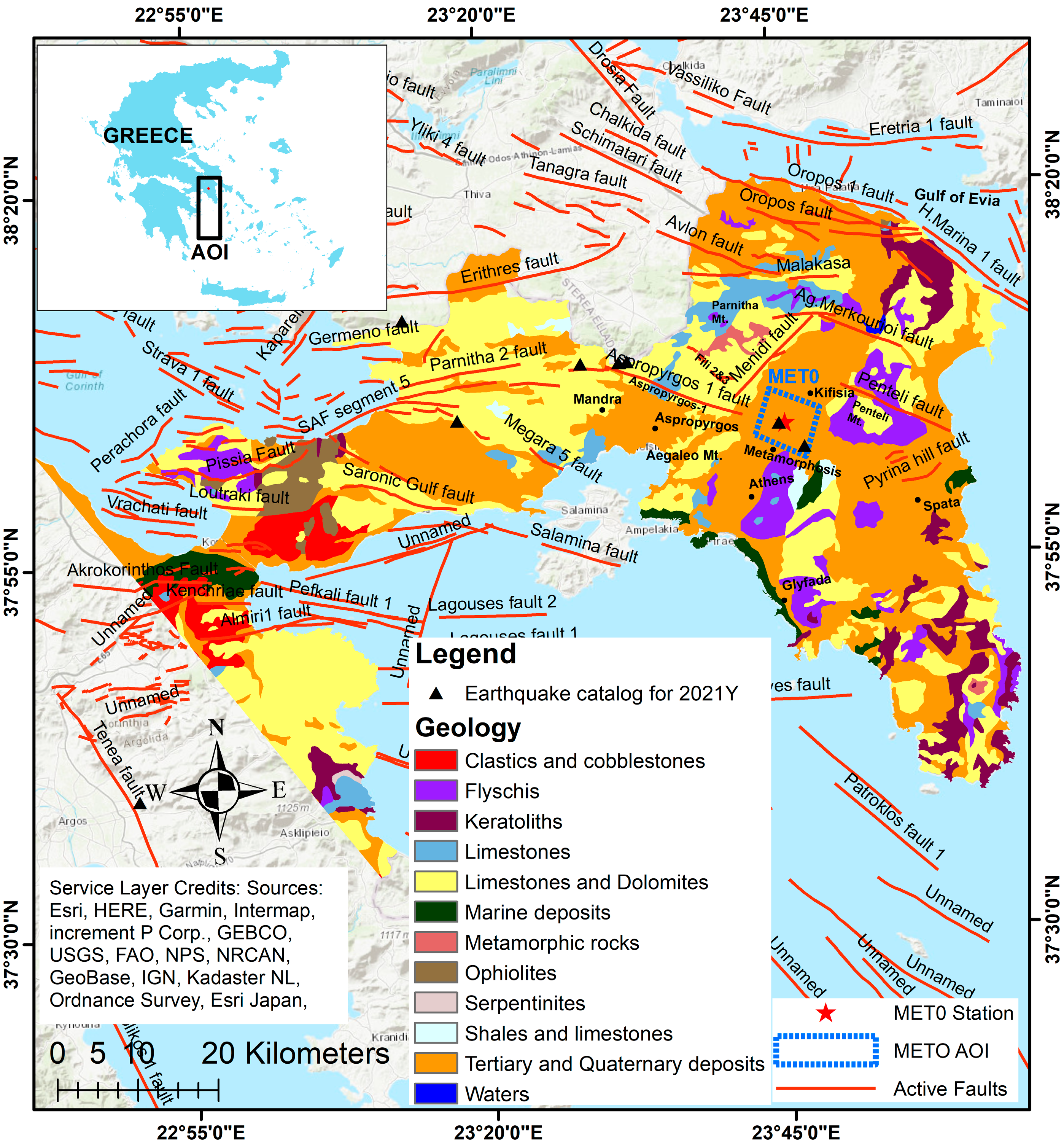
2.1. Geological and Seismic Context of Northern Attica
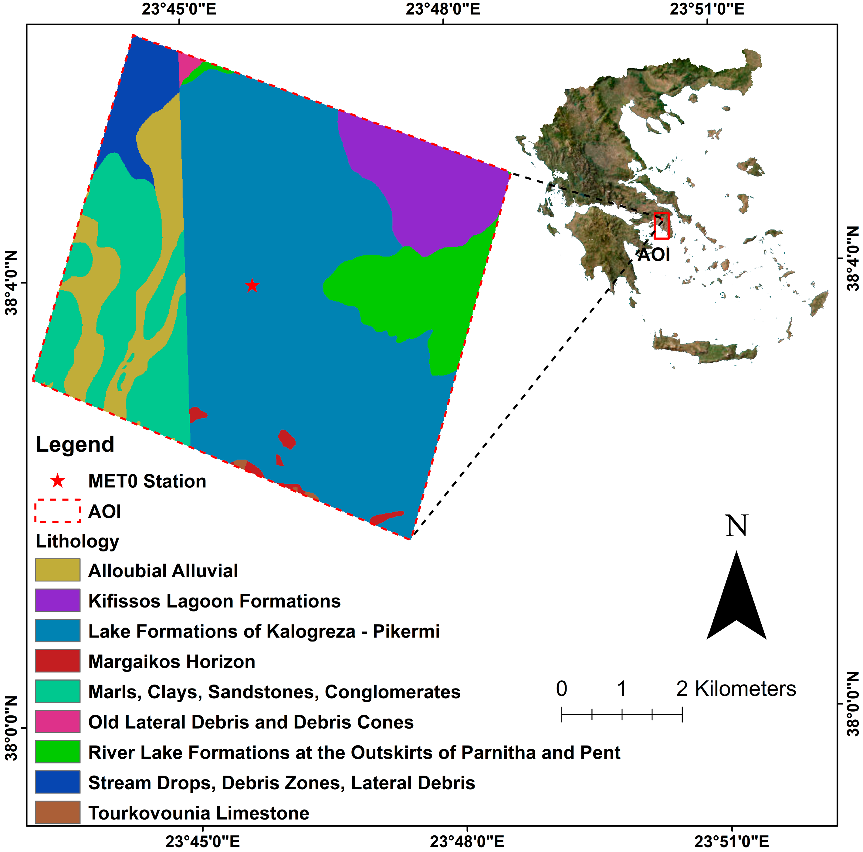
2.2. Lithological Context of Area of Interest
3. Materials and Methods
3.1. Dataset Used
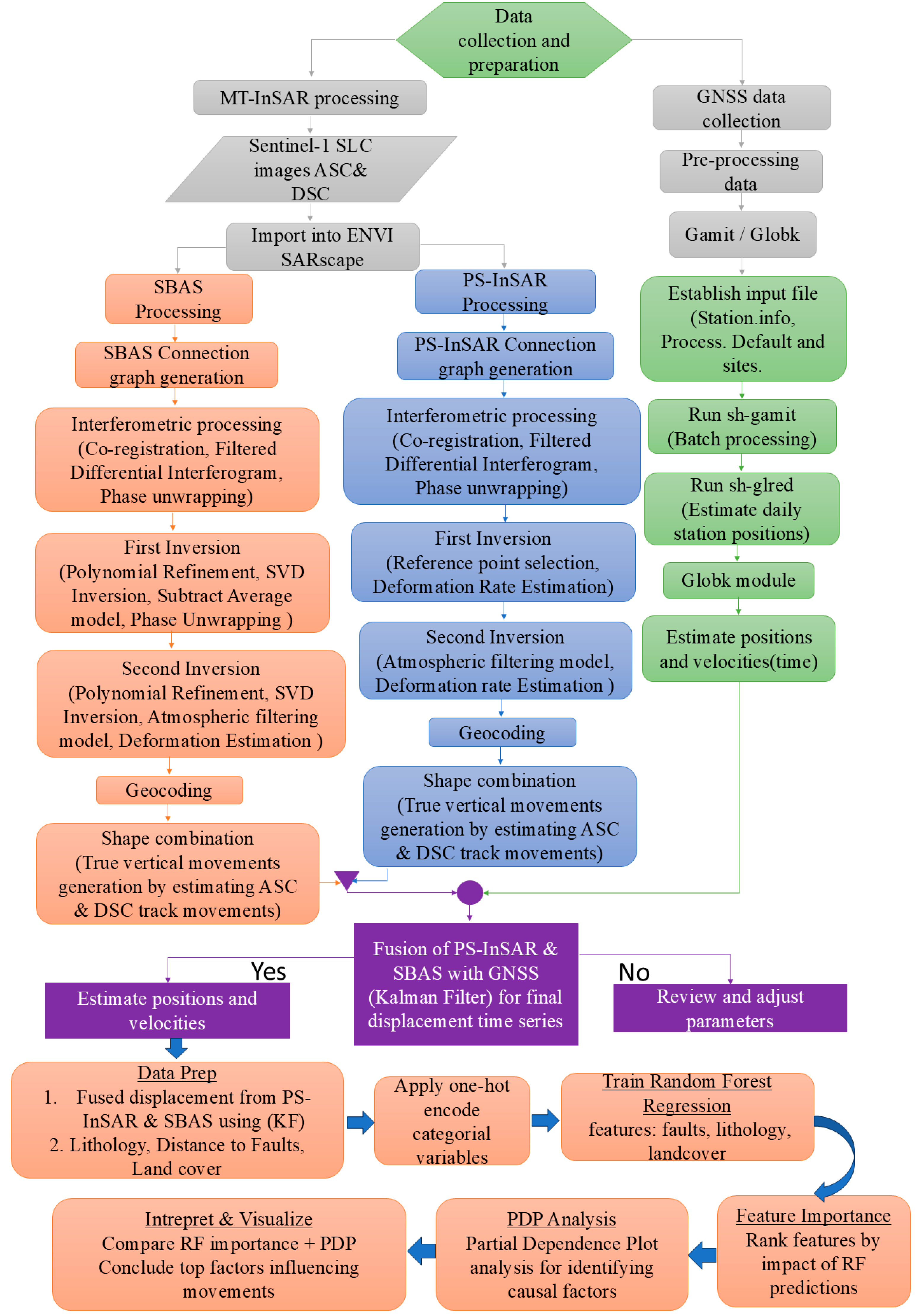
3.2. Methods
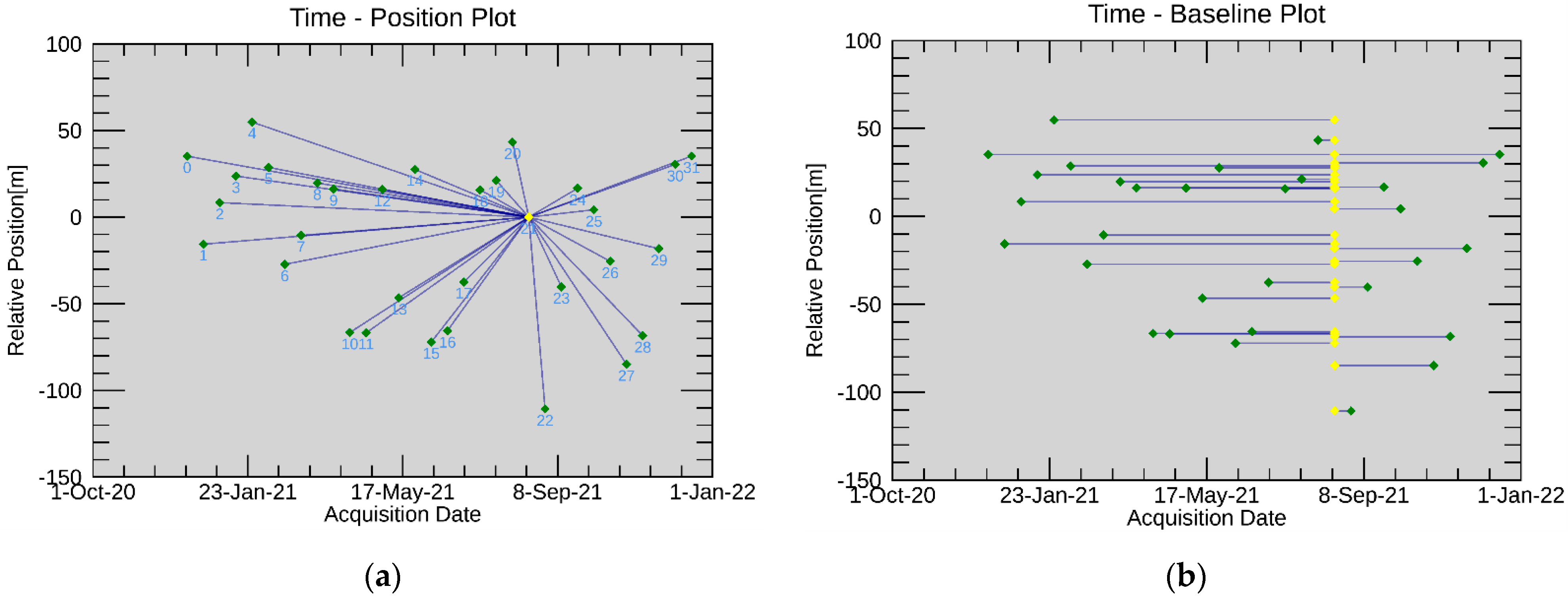
3.2.1. PS-InSAR Processing
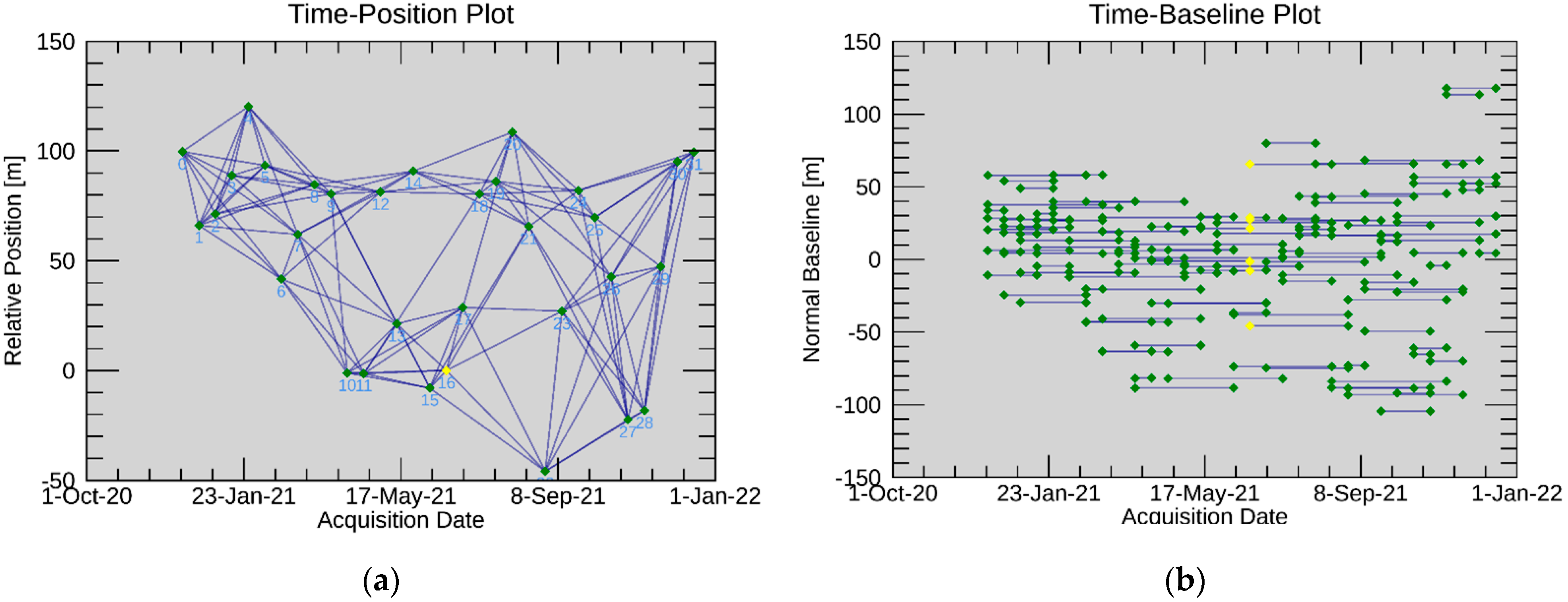
3.2.2. SBAS Processing
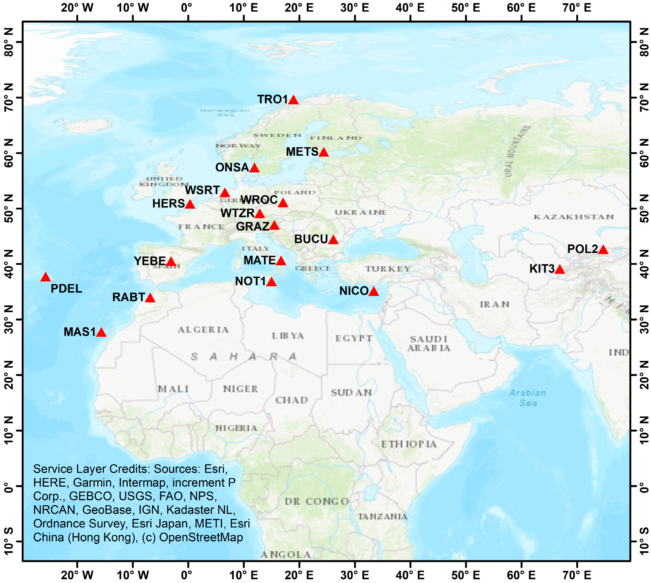
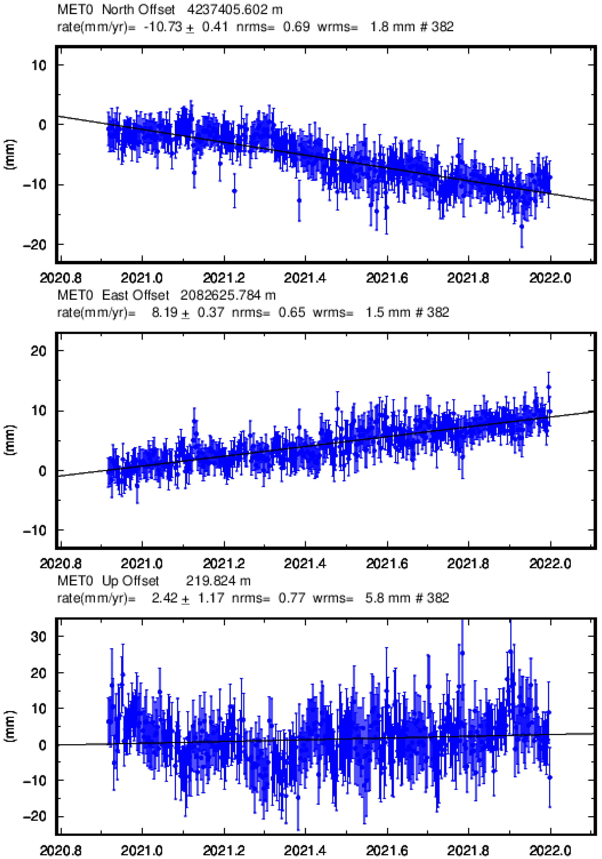
3.2.3. GNSS Data Processing
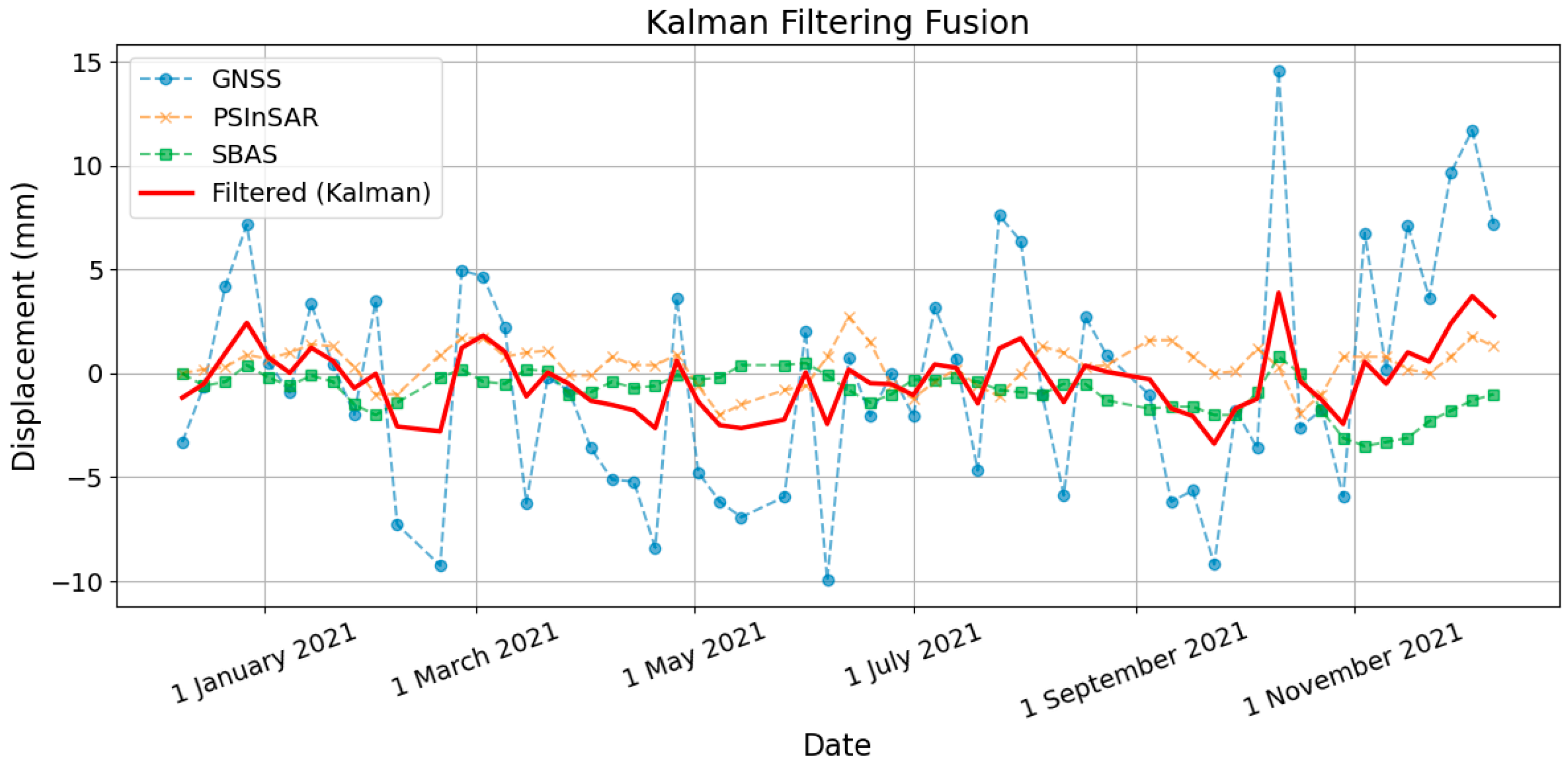
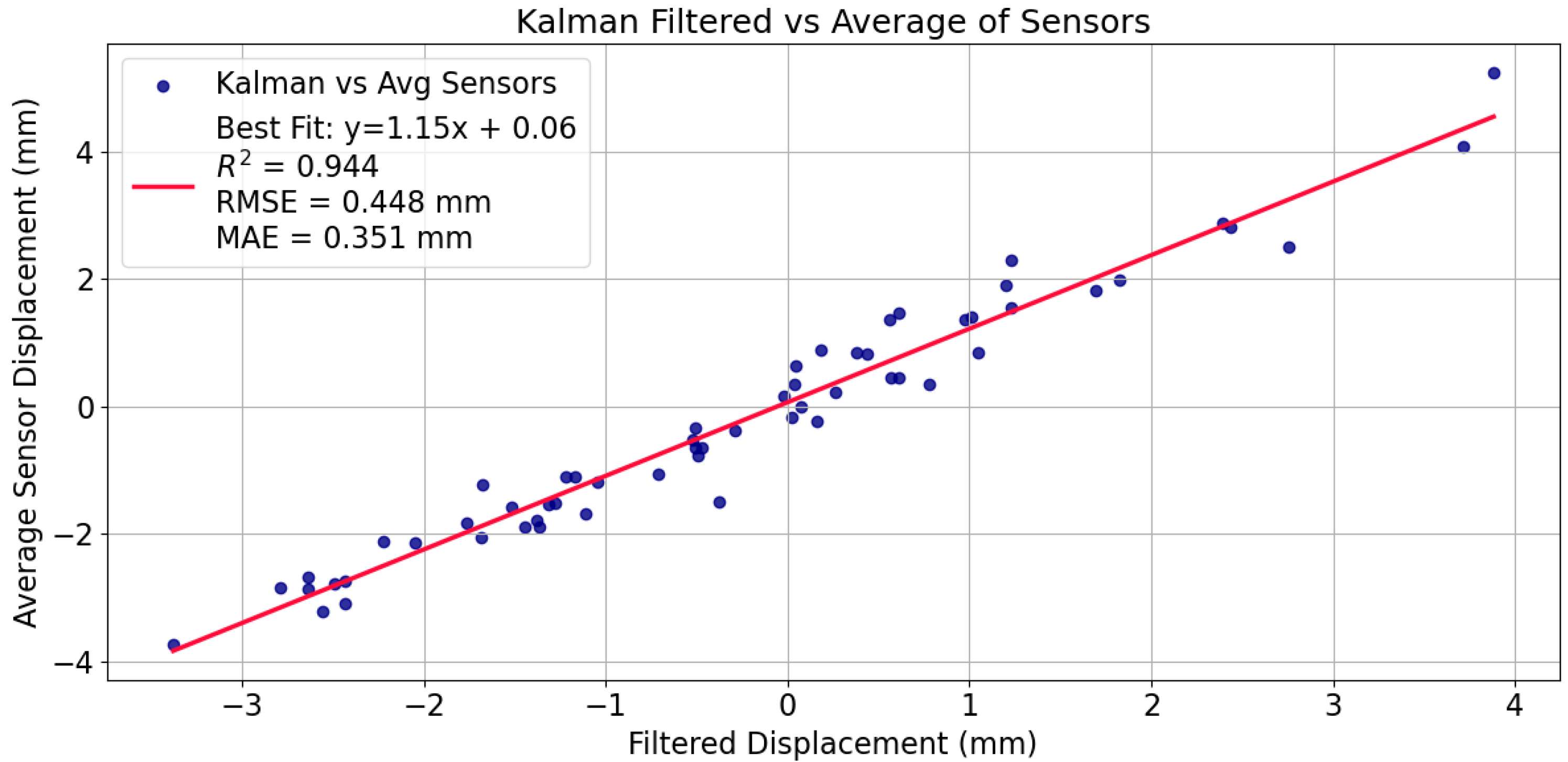
3.2.4. GNSS Kalman Filtering Fusion of GNSS, Ps-InSAR, and SBAS Displacement
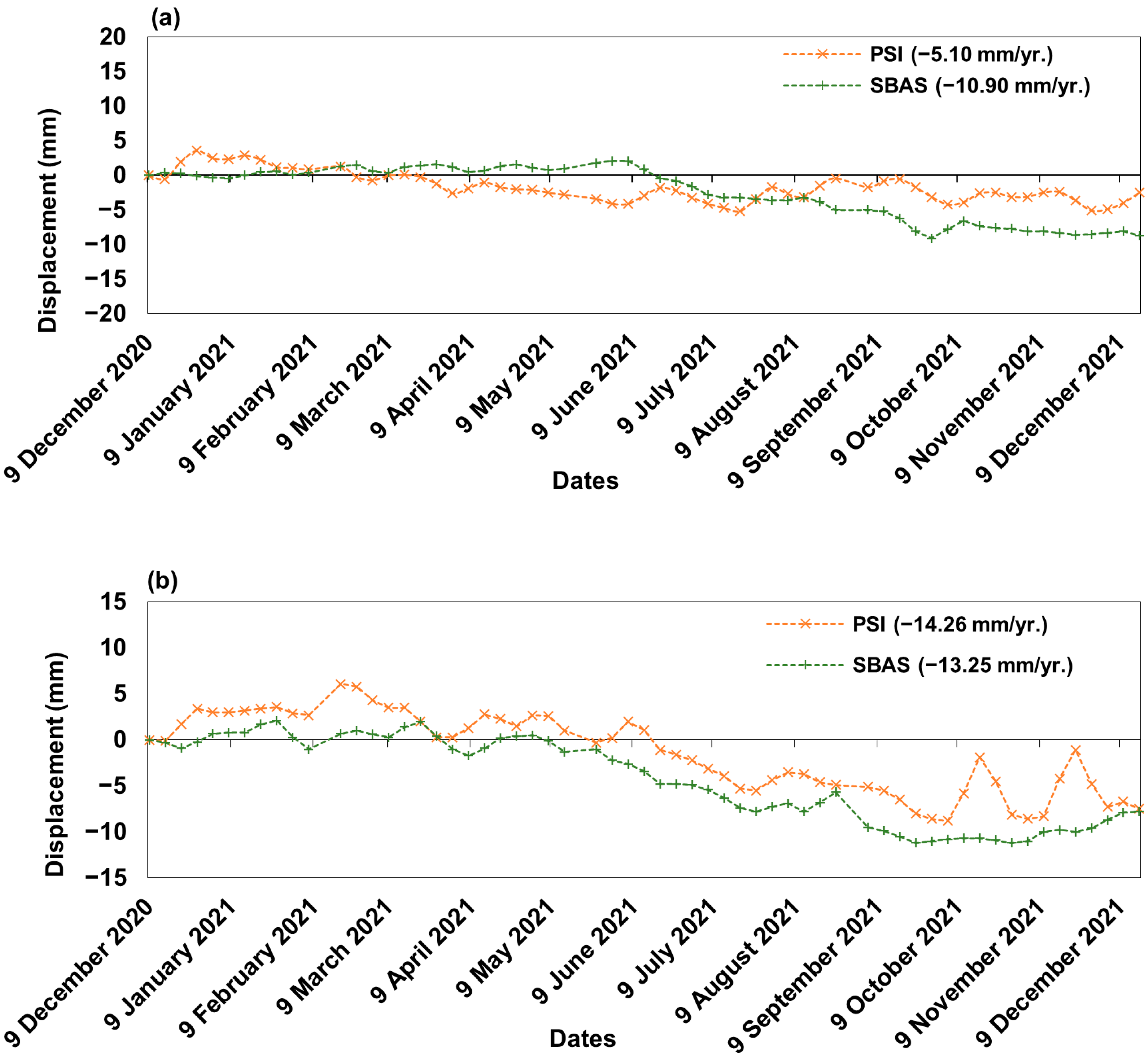
3.2.5. Kalman Filtering Fusion of PS-InSAR and SBAS to Estimate High Accuracy Displacement
3.2.6. Feature Importance and Partial Dependence Analysis
4. Results
5. Discussion
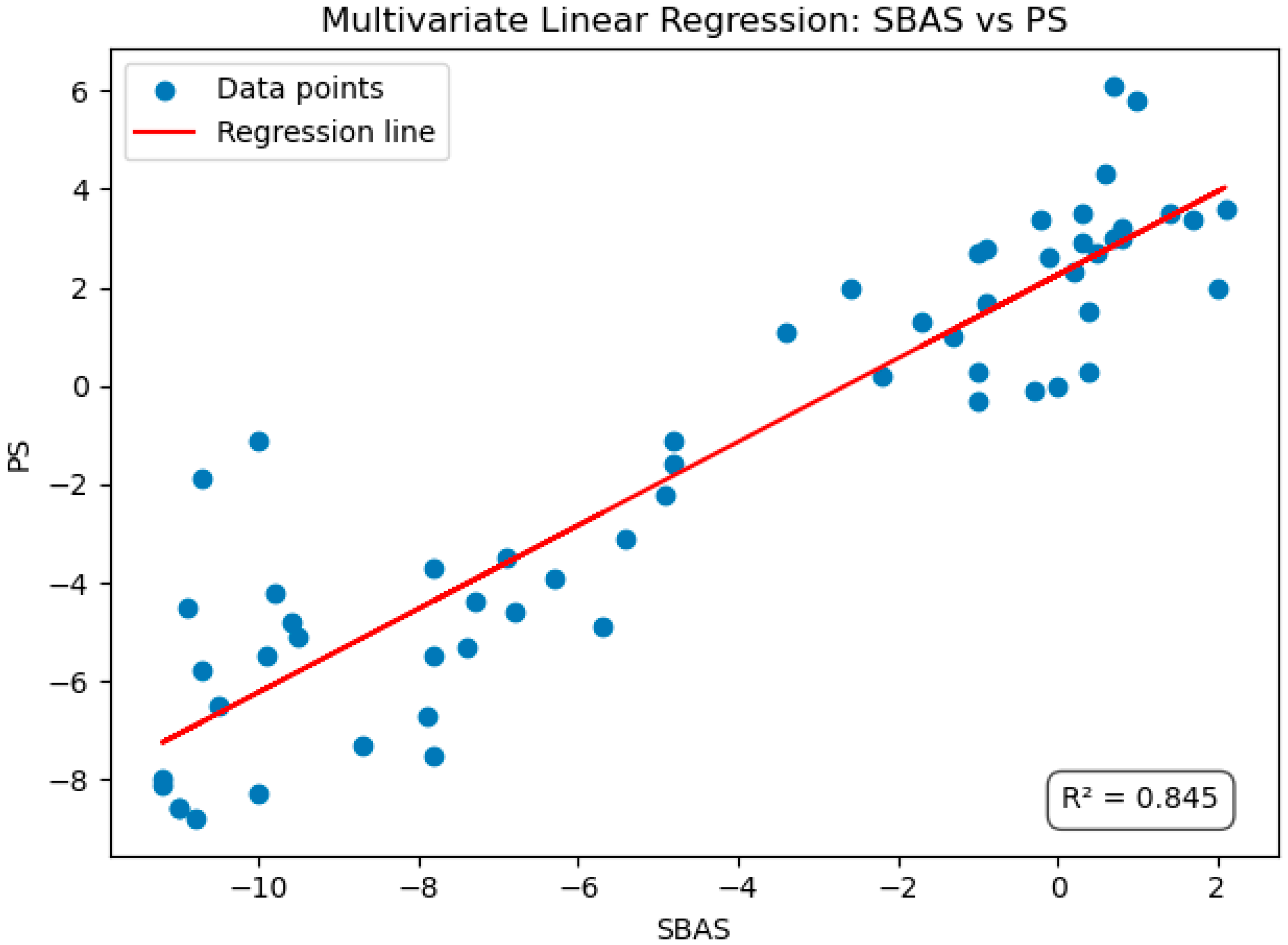
5.1. Fusion of PS-InSAR and SBAS
5.2. Feature Importance Regression Analysis and Causal Factors
6. Conclusions
Author Contributions
Funding
Data Availability Statement
Acknowledgments
Conflicts of Interest
Appendix A
References
- Zhou, C.; Gong, H.; Chen, B.; Gao, M.; Cao, Q.; Cao, J.; Duan, L.; Zuo, J.; Shi, M. Land Subsidence Response to Different Land Use Types and Water Resource Utilization in Beijing-Tianjin-Hebei, China. Remote Sens. 2020, 12, 457. [Google Scholar] [CrossRef]
- Holzer, T.L.; Galloway, D.L. Impacts of Land Subsidence Caused by Withdrawal of Underground Fluids in the United States. In Humans as Geologic Agents; Ehlen, J., Haneberg, W.C., Larson, R.A., Eds.; Geological Society of America: Boulder, CO, USA, 2005; Volume 16, p. 14. ISBN 978-0-8137-4116-1. [Google Scholar]
- Arabameri, A.; Saha, S.; Roy, J.; Tiefenbacher, J.P.; Cerda, A.; Biggs, T.; Pradhan, B.; Thi Ngo, P.T.; Collins, A.L. A Novel Ensemble Computational Intelligence Approach for the Spatial Prediction of Land Subsidence Susceptibility. Sci. Total Environ. 2020, 726, 138595. [Google Scholar] [CrossRef] [PubMed]
- Raspini, F.; Bianchini, S.; Moretti, S.; Loupasakis, C.; Rozos, D.; Duro, J.; Garcia, M. Advanced Interpretation of Interferometric SAR Data to Detect, Monitor and Model Ground Subsidence: Outcomes from the ESA-GMES Terrafirma Project. Nat. Hazards 2016, 83, 155–181. [Google Scholar] [CrossRef]
- Ganas, A.; Elias, P.; Kapetanidis, V.; Valkaniotis, S.; Briole, P.; Kassaras, I.; Argyrakis, P.; Barberopoulou, A.; Moshou, A. The July 20, 2017 M6.6 Kos Earthquake: Seismic and Geodetic Evidence for an Active North-Dipping Normal Fault at the Western End of the Gulf of Gökova (SE Aegean Sea). Pure Appl. Geophys. 2019, 176, 4177–4211. [Google Scholar] [CrossRef]
- Ganas, A.; Briole, P.; Bozionelos, G.; Barberopoulou, A.; Elias, P.; Tsironi, V.; Valkaniotis, S.; Moshou, A.; Mintourakis, I. The 25 October 2018 Mw = 6.7 Zakynthos Earthquake (Ionian Sea, Greece): A Low-Angle Fault Model Based on GNSS Data, Relocated Seismicity, Small Tsunami and Implications for the Seismic Hazard in the West Hellenic Arc. J. Geodyn. 2020, 137, 101731. [Google Scholar] [CrossRef]
- Argyrakis, P.; Ganas, A.; Valkaniotis, S.; Tsioumas, V.; Sagias, N.; Psiloglou, B. Anthropogenically Induced Subsidence in Thessaly, Central Greece: New Evidence from GNSS Data. Nat. Hazards 2020, 102, 179–200. [Google Scholar] [CrossRef]
- Ustun, A.; Tusat, E.; Yalvac, S. Preliminary Results of Land Subsidence Monitoring Project in Konya Closed Basin between 2006–2009 by Means of GNSS Observations. Nat. Hazards Earth Syst. Sci. 2010, 10, 1151–1157. [Google Scholar] [CrossRef]
- Abidin, H.Z.; Andreas, H.; Gamal, M.; Djaja, R.; Subarya, C.; Hirose, K.; Maruyama, Y.; Murdohardono, D.; Rajiyowiryono, H. Monitoring Land Subsidence of Jakarta (Indonesia) Using Leveling, GPS Survey and InSAR Techniques. In A Window on the Future of Geodesy: Proceedings of the International Association of Geodesy IAG General Assembly, Sapporo, Japan, 30 June–11 July 2003; Springer: Berlin/Heidelberg, Germany, 2005; pp. 561–566. [Google Scholar]
- Haas, R. COLDMAGICS–Continuous Local Deformation Monitoring of an Arctic Geodetic Fundamental Station. In Proceedings of the Sixth General Meeting of the International VLBI Service for Geodesy and Astrometry, Hobart, Australia, 7–13 February 2010. [Google Scholar]
- Kaloop, M.R.; Beshr, A.A.; Elshiekh, M.Y. Using Total Station for Monitoring the Deformation of High Strength Concrete Beams. In Proceedings of the 6th International Conference on Vibration Engineering (ICVE 2008), Dalian, China, 4–5 June 2008; pp. 411–419. [Google Scholar]
- Hu, B.; Chen, J.; Zhang, X. Monitoring the Land Subsidence Area in a Coastal Urban Area with InSAR and GNSS. Sensors 2019, 19, 3181. [Google Scholar] [CrossRef]
- Piras, M.; Roggero, M.; Fantino, M. Crustal Deformation Monitoring by GNSS: Network Analysis and Case Studies. Adv. Geosci. 2024, 13, 87–103. [Google Scholar] [CrossRef]
- Duong, T.T. Real-Time Deformation Monitoring with Clustered GNSS RTK Networks: An Advanced CORS Approach for Structural Stability Analysis. In Proceedings of the Geoinformatics for Spatial-Infrastructure Development in Earth and Allied Sciences, Ha Noi, Vietnam, 7–9 November 2023; Bui, D.T., Hoang, A.H., Le, T.T., Vu, D.T., Raghavan, V., Eds.; Springer Nature: Cham, Switzerland, 2024; pp. 362–380. [Google Scholar]
- Huang, G.; Du, S.; Wang, D. GNSS Techniques for Real-Time Monitoring of Landslides: A Review. Satell. Navig. 2023, 4, 5. [Google Scholar] [CrossRef]
- Berardino, P.; Fornaro, G.; Lanari, R.; Sansosti, E. A New Algorithm for Surface Deformation Monitoring Based on Small Baseline Differential SAR Interferograms. IEEE Trans. Geosci. Remote Sens. 2002, 40, 2375–2383. [Google Scholar] [CrossRef]
- Perissin, D.; Wang, T. Time-Series InSAR Applications Over Urban Areas in China. IEEE J. Sel. Top. Appl. Earth Obs. Remote Sens. 2011, 4, 92–100. [Google Scholar] [CrossRef]
- Herrera, G.; Gutiérrez, F.; García-Davalillo, J.C.; Guerrero, J.; Notti, D.; Galve, J.P.; Fernández-Merodo, J.A.; Cooksley, G. Multi-Sensor Advanced DInSAR Monitoring of Very Slow Landslides: The Tena Valley Case Study (Central Spanish Pyrenees). Remote Sens. Environ. 2013, 128, 31–43. [Google Scholar] [CrossRef]
- Ferretti, A.; Savio, G.; Barzaghi, R.; Borghi, A.; Musazzi, S.; Novali, F.; Prati, C.; Rocca, F. Submillimeter Accuracy of InSAR Time Series: Experimental Validation. IEEE Trans. Geosci. Remote Sens. 2007, 45, 1142–1153. [Google Scholar] [CrossRef]
- Zhou, W.; Lowry, B.; Wnuk, K.; Liu, L.; Gutierrez, M. InSAR and Its Applications in Geo-Engineering: Case Studies with Different Platforms and Sensors. In Proceedings of the Information Technology in Geo-Engineering, Golden, CO, USA, 5–8 August 2024; Gutierrez, M., Ed.; Springer Nature: Cham, Switzerland, 2025; pp. 175–186. [Google Scholar]
- Zhou, X.; Chang, N.-B.; Li, S. Applications of SAR Interferometry in Earth and Environmental Science Research. Sensors 2009, 9, 1876–1912. [Google Scholar] [CrossRef]
- Shanker, P.; Casu, F.; Zebker, H.A.; Lanari, R. Comparison of Persistent Scatterers and Small Baseline Time-Series InSAR Results: A Case Study of the San Francisco Bay Area. IEEE Geosci. Remote Sens. Lett. 2011, 8, 592–596. [Google Scholar] [CrossRef]
- Ferretti, A.; Prati, C.; Rocca, F. Permanent Scatterers in SAR Interferometry. IEEE Trans. Geosci. Remote Sens. 2001, 39, 8–20. [Google Scholar] [CrossRef]
- Lanari, R.; Lundgren, P.; Manzo, M.; Casu, F. Satellite Radar Interferometry Time Series Analysis of Surface Deformation for Los Angeles, California. Geophys. Res. Lett. 2004, 31, 23. [Google Scholar] [CrossRef]
- Betz, J.W. Satellite-Based Augmentation Systems. In Engineering Satellite-Based Navigation and Timing: Global Navigation Satellite Systems, Signals, and Receivers; IEEE: Piscataway, NJ, USA, 2016; pp. 201–211. ISBN 978-1-118-61593-5. [Google Scholar]
- Chen, X.; Tessari, G.; Fabris, M.; Achilli, V.; Floris, M. Comparison Between PS and SBAS InSAR Techniques in Monitoring Shallow Landslides. In Understanding and Reducing Landslide Disaster Risk; ICL Contribution to Landslide Disaster Risk Reduction; Springer International Publishing: Cham, Switzerland, 2021; pp. 155–161. ISBN 978-3-030-60310-6. [Google Scholar]
- Hooper, A. A Multi-Temporal InSAR Method Incorporating Both Persistent Scatterer and Small Baseline Approaches. Geophys. Res. Lett. 2008, 35, 654. [Google Scholar] [CrossRef]
- Lanari, R.; Mora, O.; Manunta, M.; Mallorqui, J.J.; Berardino, P.; Sansosti, E. A Small-Baseline Approach for Investigating Deformations on Full-Resolution Differential SAR Interferograms. IEEE Trans. Geosci. Remote Sens. 2004, 42, 1377–1386. [Google Scholar] [CrossRef]
- Zhou, L.; Guo, J.M.; Li, X. Monitoring and Analyzing Surface Subsidence Based on SBAS-InSAR in Beijing Region, China. In Proceedings of the International Conference on Intelligent Earth Observing and Applications, Guilin, China, 23–24 October 2015; Volume 9808. [Google Scholar]
- Wang, S.; Zhang, G.; Chen, Z.; Cui, H.; Zheng, Y.; Xu, Z.; Li, Q. Surface Deformation Extraction from Small Baseline Subset Synthetic Aperture Radar Interferometry (SBAS-InSAR) Using Coherence-Optimized Baseline Combinations. GIScience Remote Sens. 2022, 59, 295–309. [Google Scholar] [CrossRef]
- Li, S.; Xu, W.; Li, Z. Review of the SBAS InSAR Time-Series Algorithms, Applications, and Challenges. Geod. Geodyn. 2022, 13, 114–126. [Google Scholar] [CrossRef]
- Fabris, M.; Battaglia, M.; Chen, X.; Menin, A.; Monego, M.; Floris, M. An Integrated InSAR and GNSS Approach to Monitor Land Subsidence in the Po River Delta (Italy). Remote Sens. 2022, 14, 5578. [Google Scholar] [CrossRef]
- Kakar, N.; Zhao, C.; Li, G.; Zhao, H. GNSS and Sentinel-1 InSAR Integrated Long-Term Subsidence Monitoring in Quetta and Mastung Districts, Balochistan, Pakistan. Remote Sens. 2024, 16, 1521. [Google Scholar] [CrossRef]
- Kalman, R.E. A New Approach to Linear Filtering and Prediction Problems. J. Basic Eng. 1960, 82, 35–45. [Google Scholar] [CrossRef]
- Deng, Z.-L.; Gao, Y.; Mao, L.; Li, Y.; Hao, G. New Approach to Information Fusion Steady-State Kalman Filtering. Automatica 2005, 41, 1695–1707. [Google Scholar] [CrossRef]
- Fatehi, A.; Huang, B. Kalman Filtering Approach to Multi-Rate Information Fusion in the Presence of Irregular Sampling Rate and Variable Measurement Delay. J. Process Control 2017, 53, 15–25. [Google Scholar] [CrossRef]
- Xu, J.; Huang, G.; Yu, W.; Zhang, X.; Zhao, L.; Li, R.; Yuan, S.; Xie, L. Selective Kalman Filter: When and How to Fuse Multi-Sensor Information to Overcome Degeneracy in SLAM. arXiv 2024, arXiv:2412.17235. [Google Scholar]
- Saarela, M.; Jauhiainen, S. Comparison of Feature Importance Measures as Explanations for Classification Models. SN Appl. Sci. 2021, 3, 272. [Google Scholar] [CrossRef]
- Rakhimberdieva, M.; Makhmudov, M.; Fazilova, D.; Magdiev, H. Processing of GNSS Data in Gamit/Globk: On the Example of the Reference Stations of the Uzbekistan Network. E3S Web Conf. 2023, 386, 04005. [Google Scholar] [CrossRef]
- Vujinović, M.; Bulatovic, V.; Ćatić, J.; Batilović, M.; Davidovic Manojlović, M. GAMIT/GLOBK: A Review of Methodology, Applications, and Future Perspectives. In Proceedings of the 9th International Conference “Civil Engineering—Science And Practice” GNP 2024, Kolašin, Montenegro, 5–9 March 2024. [Google Scholar]
- Li, Y. Analysis of GAMIT/GLOBK in High-Precision GNSS Data Processing for Crustal Deformation. Earthq. Res. Adv. 2021, 1, 100028. [Google Scholar] [CrossRef]
- Deligiannakis, G.; Papanikolaou, I.D.; Roberts, G. Fault Specific GIS Based Seismic Hazard Maps for the Attica Region, Greece. Geomorphology 2018, 306, 264–282. [Google Scholar] [CrossRef]
- Tavoularis, N.; Papathanassiou, G.; Ganas, A.; Argyrakis, P. Development of the Landslide Susceptibility Map of Attica Region, Greece, Based on the Method of Rock Engineering System. Land 2021, 10, 148. [Google Scholar] [CrossRef]
- Ganas, A.; Pavlides, S.B.; Sboras, S.; Valkaniotis, S.; Papaioannou, S.; Alexandris, G.A.; Plessa, A.; Papadopoulos, G.A. Active Fault Geometry and Kinematics in Parnitha Mountain, Attica, Greece. J. Struct. Geol. 2004, 26, 2103–2118. [Google Scholar] [CrossRef]
- Ganas, A.; Pavlides, S.; Karastathis, V. DEM-Based Morphometry of Range-Front Escarpments in Attica, Central Greece, and Its Relation to Fault Slip Rates. Geomorphology 2005, 65, 301–319. [Google Scholar] [CrossRef]
- Grützner, C.; Schneiderwind, S.; Papanikolaou, I.; Deligiannakis, G.; Pallikarakis, A.; Reicherter, K. New Constraints on Extensional Tectonics and Seismic Hazard in Northern Attica, Greece: The Case of the Milesi Fault. Geophys. J. Int. 2016, 204, 180–199. [Google Scholar] [CrossRef]
- Drakatos, G.; Melis, N.; Papanastassiou, D.; Karastathis, V.; Papadopoulos, G.A.; Stavrakakis, G. 3-D Crustal Velocity Structure from Inversion of Local Earthquake Data in Attiki (Central Greece) Region. Nat. Hazards 2002, 27, 1–14. [Google Scholar] [CrossRef]
- Drakatos, G.; Karastathis, V.; Makris, J.; Papoulia, J.; Stavrakakis, G. 3D Crustal Structure in the Neotectonic Basin of the Gulf of Saronikos (Greece). Tectonophysics 2005, 400, 55–65. [Google Scholar] [CrossRef]
- Ganas, A. NOAFAULTS KMZ Layer, Version 5.0; Zenodo: Athens, Greece, 2023.
- Crosetto, M.; Devanthéry, N.; Cuevas-González, M.; Monserrat, O.; Crippa, B. Exploitation of the Full Potential of PSI Data for Subsidence Monitoring. Proc. IAHS 2015, 372, 311–314. [Google Scholar] [CrossRef]
- Hooper, A.; Zebker, H.; Segall, P.; Kampes, B. A New Method for Measuring Deformation on Volcanoes and Other Natural Terrains Using InSAR Persistent Scatterers. Geophys. Res. Lett. 2004, 31, 737. [Google Scholar] [CrossRef]
- Torres, R.; Snoeij, P.; Geudtner, D.; Bibby, D.; Davidson, M.; Attema, E.; Potin, P.; Rommen, B.; Floury, N.; Brown, M.; et al. GMES Sentinel-1 Mission. Remote Sens. Environ. 2012, 120, 9–24. [Google Scholar] [CrossRef]
- Adam, N.; González, F.R.; Parizzi, A.; Liebhart, W. Wide Area Persistent Scatterer Interferometry: Algorithms and Examples. In Proceedings of the 2013 IEEE International Geoscience and Remote Sensing Symposium—IGARSS, Melbourne, VIC, Australia, 21–26 July 2013. [Google Scholar]
- Parcharidis, I.; Loupasakis, C.; Kaitantzian, A. Land subsidence phenomena in urbanized areas of Attica observed by applying advanced DinSAR techniques. In Proceedings of the Fifth International Conference on Remote Sensing and Geoinformation of the Environment (RSCy2017), Paphos, Cyprus, 20–23 March 2017. [Google Scholar]
- Hou, J.; Xu, B.; Li, Z.; Zhu, Y.; Feng, G. Block PS-InSAR Ground Deformation Estimation for Large-Scale Areas Based on Network Adjustment. J. Geod. 2021, 95, 111. [Google Scholar] [CrossRef]
- Cigna, F.; Esquivel Ramírez, R.; Tapete, D. Accuracy of Sentinel-1 PSI and SBAS InSAR Displacement Velocities against GNSS and Geodetic Leveling Monitoring Data. Remote Sens. 2021, 13, 4800. [Google Scholar] [CrossRef]
- Zhang, Y.; Liu, Y.; Jin, M.; Jing, Y.; Liu, Y.; Liu, Y.; Sun, W.; Wei, J.; Chen, Y. Monitoring Land Subsidence in Wuhan City (China) Using the SBAS-InSAR Method with Radarsat-2 Imagery Data. Sensors 2019, 19, 743. [Google Scholar] [CrossRef]
- Feng, Q.; Xu, H.; Wu, Z.; You, Y.; Liu, W.; Ge, S. Improved Goldstein Interferogram Filter Based on Local Fringe Frequency Estimation. Sensors 2016, 16, 1976. [Google Scholar] [CrossRef]
- Lin, Z.; Duan, Y.; Deng, Y.; Tian, W.; Zhao, Z. An Improved Multi-Baseline Phase Unwrapping Method for GB-InSAR. Remote Sens. 2022, 14, 2543. [Google Scholar] [CrossRef]
- Vaka, D.S.; Yaragunda, V.R.; Perdikou, S.; Papanicolaou, A. InSAR Integrated Machine Learning Approach for Landslide Susceptibility Mapping in California. Remote Sens. 2024, 16, 3574. [Google Scholar] [CrossRef]
- Bitharis, S.; Pikridas, C.; Fotiou, A.; Rossikopoulos, D. GPS Data Analysis and Geodetic Velocity Field Investigation in Greece, 2001–2016. GPS Solut 2023, 28, 16. [Google Scholar] [CrossRef]
- Amighpey, M.; Arabi, S. Studying Land Subsidence in Yazd Province, Iran, by Integration of InSAR and Levelling Measurements. Remote Sens. Appl. Soc. Environ. 2016, 4, 1–8. [Google Scholar] [CrossRef]
- Motagh, M.; Djamour, Y.; Walter, T.R.; Wetzel, H.-U.; Zschau, J.; Arabi, S. Land Subsidence in Mashhad Valley, Northeast Iran: Results from InSAR, Levelling and GPS. Geophys. J. Int. 2007, 168, 518–526. [Google Scholar] [CrossRef]
- Delen, A.; Sanli, F.B.; Abdikan, S.; Dogan, A.H.; Durdag, U.M.; Ocalan, T.; Erdogan, B.; Calò, F.; Pepe, A. A Statistical Approach for the Integration of Multi-Temporal InSAR and GNSS-PPP Ground Deformation Measurements. Sensors 2024, 24, 43. [Google Scholar] [CrossRef] [PubMed]
- Yan, H.; Dai, W.; Xu, W.; Shi, Q.; Sun, K.; Lu, Z.; Wang, R. A Method for Correcting InSAR Interferogram Errors Using GNSS Data and the K-Means Algorithm. Earth Planets Space 2024, 76, 51. [Google Scholar] [CrossRef]
- Brown, R.G.; Hwang, P.Y.C. Introduction to Random Signals and Applied Kalman Filtering with Matlab Exercises; John Wiley & Sons: New York, NY, USA, 2012; ISBN 978-0-470-60969-9. [Google Scholar]
- Orderud, F.; Sælands, S. Comparison of Kalman Filter Estimation Approaches for State Space Models with Nonlinear Measurements. In Proceedings of the Scandinavian Conference on Simulation and Modeling, Trondheim, Norway, 13–14 October 2005. [Google Scholar]
- Tekin Ünlütürk, N.; Doğan, U. The Effect of Seasonal Variation on Gnss Zenith Tropospheric Delay. Int. Arch. Photogramm. Remote Sens. Spat. Inf. Sci. 2024, 2024, 371–376. [Google Scholar] [CrossRef]
- Chang, S.; Deng, Y.; Zhang, Y.; Zhao, Q.; Wang, R.; Zhang, K. An Advanced Scheme for Range Ambiguity Suppression of Spaceborne SAR Based on Blind Source Separation. IEEE Trans. Geosci. Remote Sens. 2022, 60, 1–12. [Google Scholar] [CrossRef]
- Sun, Z.; Leng, X.; Zhang, X.; Zhou, Z.; Xiong, B.; Ji, K.; Kuang, G. Arbitrary-Direction SAR Ship Detection Method for Multiscale Imbalance. IEEE Trans. Geosci. Remote Sens. 2025, 63, 1–21. [Google Scholar] [CrossRef]
- Krohe, A.; Mposkos, E.; Diamantopoulos, A.; Kaouras, G. Formation of Basins and Mountain Ranges in Attica (Greece): The Role of Miocene to Recent Low-Angle Normal Detachment Faults. Earth-Sci. Rev. 2010, 98, 81–104. [Google Scholar] [CrossRef]


| Data Information | Descending | Ascending |
|---|---|---|
| No. of images | 32 | 32 |
| Period of acquisition | 3 December 2020–22 December 2021 | 9 December 2020–16 December 2021 |
| Track no. | 09 | 102 |
| Parameters | Description | |
| Product type | Sentinel-1 IW SLC | Sentinel-1 IW SLC |
| Polarization | VV+VH | VV+VH |
| Band | C | C |
| Coverage (km2) | 250 | 250 |
| Return frequency (day) | 12 | 12 |
| Range (m) | 5 | 5 |
| Azimuth resolution (m) | 20 | 20 |
Disclaimer/Publisher’s Note: The statements, opinions and data contained in all publications are solely those of the individual author(s) and contributor(s) and not of MDPI and/or the editor(s). MDPI and/or the editor(s) disclaim responsibility for any injury to people or property resulting from any ideas, methods, instructions or products referred to in the content. |
© 2025 by the authors. Licensee MDPI, Basel, Switzerland. This article is an open access article distributed under the terms and conditions of the Creative Commons Attribution (CC BY) license (https://creativecommons.org/licenses/by/4.0/).
Share and Cite
Yaragunda, V.R.; Oikonomou, E. Multi-Sensor Fusion for Land Subsidence Monitoring: Integrating MT-InSAR and GNSS with Kalman Filtering and Feature Importance to Northern Attica, Greece. Earth 2025, 6, 37. https://doi.org/10.3390/earth6020037
Yaragunda VR, Oikonomou E. Multi-Sensor Fusion for Land Subsidence Monitoring: Integrating MT-InSAR and GNSS with Kalman Filtering and Feature Importance to Northern Attica, Greece. Earth. 2025; 6(2):37. https://doi.org/10.3390/earth6020037
Chicago/Turabian StyleYaragunda, Vishnuvardhan Reddy, and Emmanouil Oikonomou. 2025. "Multi-Sensor Fusion for Land Subsidence Monitoring: Integrating MT-InSAR and GNSS with Kalman Filtering and Feature Importance to Northern Attica, Greece" Earth 6, no. 2: 37. https://doi.org/10.3390/earth6020037
APA StyleYaragunda, V. R., & Oikonomou, E. (2025). Multi-Sensor Fusion for Land Subsidence Monitoring: Integrating MT-InSAR and GNSS with Kalman Filtering and Feature Importance to Northern Attica, Greece. Earth, 6(2), 37. https://doi.org/10.3390/earth6020037