Abstract
Air pollution is among the key topics in environmental policies and mitigation policies. Governments and institutions worldwide are working towards a better understanding of the phenomenon and means to reduce its impact on the environment and human health. In early 2020, the COVID-19 pandemic forced many countries to introduce strict regulations, effectively stopping non-essential anthropic activities. Italy had a pioneering role in this regard, anticipating other countries in Europe and across the world. These exceptional circumstances caused the concentrations of pollutants in the atmosphere to reach lower levels, thus allowing researchers to evaluate a number of hypotheses concerning the contribution of anthropogenic emissions. At the Lamezia Terme (code: LMT) World Meteorological Organization—Global Atmosphere Watch (WMO/GAW) regional station in Calabria, Italy, previous research highlighted the effects of governmental restrictions on the concentrations of gases (carbon monoxide, CO; carbon dioxide, CO2; methane, CH4, nitrogen oxides, NOx) and aerosols (black carbon, BC). In this work, sulfur dioxide (SO2) and ozone (O3) are also evaluated and all parameters are subject to the analysis based on the O3/NOx ratio, the ONRPI (Ozone to Nitrogen Oxides Ratio Proximity Indicator), which has been widely used at LMT to verify the balance between local and remote sources of emission. The implementation of this method to the first 2020 COVID-19 lockdown in the country has allowed significant improvement in our understanding of the variability of all evaluated parameters at the site, assessing with greater detail weekly cycles and day–night contrasts, and the influence of local and remote sources of emission.
Keywords:
ONRPI; COVID-19; lockdown; Italy; air mass aging; carbon monoxide; carbon dioxide; methane; black carbon; sulfur dioxide; ozone; nitrogen oxides 1. Introduction
The issue of air pollution is a leading topic in scientific research due to its vast scale of impact [1,2,3,4,5,6,7,8]. According to a WHO (World Health Organization) estimate, seven million annual deaths across the globe can be attributed to the adverse effects of air pollution on human health [9]. Additionally, air pollution can impact the environment, worsening the conditions of ecosystems [10,11,12,13,14,15,16,17].
Although pollution events can occur due to natural phenomena, such as volcanic eruptions [18,19,20,21,22], a significant amount of pollutants are released into the atmosphere by anthropic activities ranging from transportation [23,24,25,26,27,28,29], the industry sector [30,31,32,33,34], mining and quarrying activities [35,36], and even agriculture, which acts as a source of pollutants and is also heavily influenced by air pollution itself [37,38,39,40,41,42]. Air pollution is known to affect indoor environments, enhanced by vastly reduced wind circulation and the presence of peculiar sources, such as furniture [43,44,45,46,47]. The need to introduce sustainable policies and reduce the effects of air pollution has led to a notable increase in the efficiency of source apportionment (SA), a process by which pollutants can be traced back to their sources [48,49,50,51,52,53]. In the field of atmospheric sciences, SA can rely on very advanced methodologies such as the analysis of stable carbon isotopes which can effectively pinpoint emission sources with greater accuracy [54,55,56]. Field activities and surveys of nearby known sources of emission can also improve the models and methods used in SA [57,58,59]. Satellite data are frequently used to assess events over large scales and compensate for the gaps left by ground observatories; however, they are affected by uncertainties in the assessment of near-surface concentrations [60,61].
In March 2020, the Italian Republic introduced very strict regulations to mitigate the COVID-19 pandemic, effectively causing activities deemed non-essential to either stop completely or be significantly reduced [62]. The pandemic and related lockdowns left a clear mark on Italy’s population and GDP [63], and the restrictions were lifted in May [64]. In the next two years, other lockdowns (LDs) occurred, but they were not as strict as the first lockdown, thus making it a unique circumstance for the assessment of SA and air quality improvement [65,66,67,68,69,70,71,72,73,74,75,76,77,78,79]. Globally, multiple studies have assessed changes in air quality and pollution during lockdowns and related measures introduced by national governments, highlighting numerous factors driving their variability over time [80,81,82].
In the southern Italian region of Calabria, the World Meteorological Organization—Global Atmosphere Watch (WMO/GAW) observation site of Lamezia Terme (code: LMT), Catanzaro province, gathered data that would consequently be used to assess the effects of the first Italian lockdown on the concentrations of carbon monoxide (CO), carbon dioxide (CO2), methane (CH4), nitrogen oxides (NOx), and black carbon (BC) [83]. In detail, the study defined the ante-lockdown (ALD), lockdown (LD), and post-lockdown (PLD) periods to discriminate anthropogenic outputs between three distinct periods in terms of anthropic activity allowed by law. The analysis exploited the exceptionally low anthropic activities of the LD period to test a number of hypotheses concerning greenhouse (GHG) and reactive (RG) gas, as well as aerosol, variability in the area. For example, the study attributed early morning peaks of NOx to rush hour traffic, as hypothesized in previous research [84]. During the LD, these emissions were nearly absent. A consequent study paired NOx data with highway traffic, showing that vehicular transit was nearly five times lower during the LD period [85]. With respect to CH4, the analysis showed no substantial reduction [83], corroborating the hypothesis by which local inputs such as livestock and agricultural farming may be responsible for peaks in CH4 [84,86].
These analyses were based on all observations at LMT, thus including outputs from both local and remote sources. Research on LMT data showed the effectiveness of the O3/NOx ratio (ONRPI, Ozone to Nitrogen Oxides Ratio Proximity Indicator) as a means to differentiate between local and remote outputs, as higher ratios are representative of more aged air masses, while lower ratios indicate fresh anthropogenic emissions [84,87]. This study is therefore aimed at applying the ONRPI to the first Italian LD period at LMT, thus marking the first attempt at using the O3/NOx ratio methodology on specific measurements characterized by very low anthropogenic emissions. This study also introduces the analysis of SO2, which was not included in previous research on the first LD at LMT.
2. The WMO/GAW Observation Site, Instruments, Datasets, and Methods
2.1. The LMT Site in the Municipality of Lamezia Terme, Catanzaro, Calabria
The Lamezia Terme (code: LMT) is a regional coastal observation site that is part of the World Meteorological Organization—Global Atmosphere Watch (WMO/GAW) network. Although it is not part of the national ICOS (Integrated Carbon Observation System) network, it operates as a “hub” supporting Italian ICOS stations. The site started its operations in 2015 in the framework of the I-AMICA (Infrastruttura di Alta tecnologia per il Monitoraggio Integrato Climatico-Ambientale, Infrastructure of High Technology for Integrated Climate and Environmental Monitoring) project [88]; however, a number of measurements were already in place as early as 2014. The station is fully operated by the National Research Council of Italy-Institute of Atmospheric Sciences and Climate (CNR-ISAC) and measures a number of meteorological and chemical parameters, ranging from wind direction/speed to greenhouse (GHG) and reactive (RG) gas concentrations. With three other stations in the country (Monte Cimone, CMN, in Northern Italy; Potenza, POT, in the neighboring region of Basilicata; and Lampedusa island, LMP, in the Strait of Sicily), LMT is part of the national consortium introducing stable carbon isotope measurements of CO2 (δ13C-CO2) and CH4 (δ13C-CH4) in the atmosphere, which are expected to improve source apportionment (SA) significantly in the framework of Italian atmospheric stations [56].
Due to its location in central Calabria (Lat: 38.8763° N; Lon: 16.2322° E; Elev: 6 m above sea level) (Figure 1A), more precisely in the westernmost area of the Catanzaro isthmus (≈32 km between the Tyrrhenian and Ionian coasts), the LMT site is heavily influenced by local near-surface wind circulation [89]. It is located 600 m from the western/Tyrrhenian coast of the region (Figure 1B), in the narrowest strip of land in the entire Italian peninsula. The geomorphology of the isthmus reflects intense tectonic activity and substantial evolution over time, as the isthmus separates two mountain ranges in the north (the Coastal Chain and Sila Massif) from the Serre Massif in the south [90,91,92,93,94,95,96,97,98,99,100,101,102,103]. In the early Quaternary, the isthmus was a tidal strait connecting the two seas [104,105,106], and the interplay of numerous factors such as the Calabrian uplift and glacial/interglacial cycles has led to the present-day configuration [107,108,109,110,111]. This also results in the area being seismically very active, with three out of ten of the strongest earthquakes in recorded Italian history (Mw ≥ 6.95, 1000 A.D. to modern times) occurring within 20 km of the current location of the LMT observation site [112,113,114].
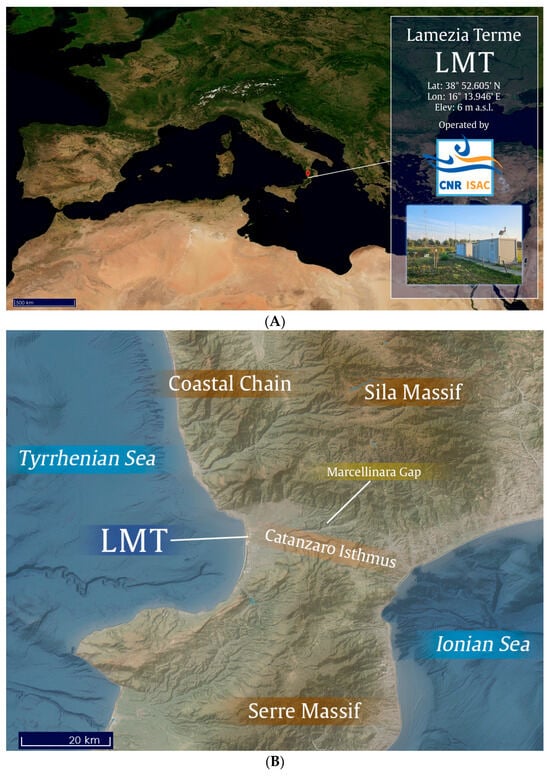
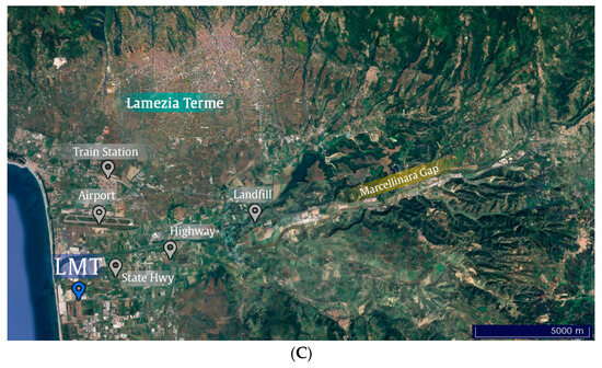
Figure 1.
(A) Location, coordinates and a picture of the LMT observatory in the broader context of the Mediterranean Basin. (B) Main geomorphological features of central Calabria, showing LMT’s location in the western sector of the Catanzaro isthmus. (C) Local map showing the municipality of Lamezia Terme, the Marcellinara Gap, and notable sources of pollution in the area.
Presently, a well-defined W-WSW/NE-ENE axis in wind circulation is reported at LMT, dominated by breeze regimes and currents being channeled through the Marcellinara Gap (Sella di Marcellinara) towards LMT (Figure 1C); when the 850 hPa layer is considered, a dominance of NW wind is reported, which is consistent with large-scale circulation patterns in the area [115,116,117]. These patterns have a prominent effect on the local variability of GHG/RGs and aerosols, as the northeastern-continental winds are generally linked to higher degrees of anthropogenic influence, while the western-seaside winds generally yield lower concentrations [84,86,87]. The Lamezia Terme International Airport (IATA: SUF; ICAO: LICA), located 3 km north of LMT station, has a 100/280° N runway orientation reflecting these wind patterns, which in turn influences local air traffic.
Various contributions and inputs of anthropogenic origin, such as those deriving from vehicular traffic and summertime tourism [118], have made LMT an ideal spot in the network of Italian atmospheric stations for the study and evaluation of anthropogenic emissions: LMT is presently the site subject to the most detailed weekly cycle analyses in the country [85,119], which are exploited to differentiate between natural and anthropogenic emissions under the assumption that the latter may show a weekly cycle, while the former would remain unaffected. Furthermore, due to its location, the site is exposed to Saharan dust intrusions [120] and open fire emissions, both on a local [121,122] and large [123] scale. The Mediterranean itself is known to be a hotspot for the impacts of climate change, environmental challenges, and air mass transport mechanisms [124,125,126,127,128,129,130,131,132,133,134,135,136,137], further contributing to the complexity of LMT’s measurements.
2.2. Parameters, Instruments, Datasets and Methods
This work evaluates carbon monoxide (CO), carbon dioxide (CO2), methane (CH4), and equivalent black carbon (eBC) measured at the Lamezia Terme (LMT) observation site between February and July 2020. These parameters are characterized by peculiar atmospheric lifetimes, balance between natural and anthropogenic sources, and specific instruments used to measure, with high precision, atmospheric concentrations.
CO (ppb), CO2 (ppm), and CH4 (ppb) concentrations have been measured by a Picarro G2401 (Santa Clara, CA, USA) CRDS (Cavity Ring-Down Spectrometry) analyzer. Details concerning these measurements at LMT, their characteristics, calibration procedures and quality assurance checks are available in Malacaria et al. [138]. Atmospheric CO is a frequent byproduct of combustion processes, such as biomass and fuel burning, and is therefore attributed to natural and anthropogenic sources alike [139,140,141]. Among the parameters considered in this study, the atmospheric lifetime of CO is intermediate (~60 days) [142] and reflects the role played by this compound in atmospheric chemistry [143,144]. Following decades of sharp increase due to anthropogenic emissions [145], CO is now characterized by a declining trend [146], punctuated by new peaks in the past few years [147,148,149]. CO2 is the main driver of anthropogenic climate change, characterized by clear upward trends driven by fossil fuel burning [150,151,152,153,154,155], and its effects are exacerbated by a very long atmospheric lifetime, potentially reaching 1000 years [156]. CH4 is relatively long-lived, with its atmospheric lifetime being ~10 years [157,158,159]; it is characterized by a clear upward trend driven by anthropic activity and a recent increase in natural emissions such as wetlands [160,161,162].
Atmospheric mole fractions of SO2 (ppb) at LMT have been measured using a Thermo Scientific 43i (Franklin, MA, USA) analyzer. Details concerning these measurements at the observation site of Lamezia Terme are available in previous research [163]. SO2 is emitted by natural and anthropogenic sources, such as volcanoes and maritime shipping [18,164,165,166,167,168,169]. The atmospheric lifetime of SO2 is very short, in the order of two days [170], partially compensating for the adverse effects of SO2 on human health [171,172,173,174,175].
A Thermo Scientific 5012 MAAP (Multi-Angle Absorption Photometer) (Franklin, MA, USA) analyzer has been used to measure equivalent black carbon [176] at LMT. Details concerning MAAP measurements at the site are available in previous works [121,177]. Black carbon is an effective tracer of combustion in the atmosphere [141,178,179], posing a tangible hazard for human health [180,181]. The atmospheric lifetime of BC is in the order of 4–12 days [182,183].
Air mass aging and proximity categories have been calculated based on O3 and NOx measurements at LMT performed by Thermo Scientific models 49i and 42i (Franklin, MA, USA), respectively. Details concerning these measurements and the implementation of the ONRPI methodology to assess air mass aging indicators are available in previous research [85,87,184]. Table 1 shows the coverage rates of all employed instruments during the study period.

Table 1.
Coverage rates of all data during the study period. The datasets are identified as follows: G2401 (Picarro G2401 CRDS analyzer for CO, CO2, CH4); T43i (Thermo Scientific 43i analyzer for SO2); MAAP (Thermo Scientific 5012 MAAP for eBC); CProx, SProx, and BProx refer to the combined datasets of valid O3/NOx ratios combined with G2401, T43i, MAAP, and meteo data. The three periods are identified as follows: ALD (ante-lockdown, 1 February–8 March); LD (lockdown, 9 March–18 May); PLD (post-lockdown, 19 May–31 July).
The ONRPI methodology used at LMT is an expansion of the methods seen in the literature, combining multiple air mass aging and proximity categories and introducing a more consistent naming convention. The O3/NOx ratio was found to be an effective tracer of air mass aging in the studies performed by Parrish et al. (2009) [185] and Morgan et al. (2010) [186]. Over time, studies such as McMeeking et al. (2010) [187], Cristofanelli et al. (2016) [188], and Ham et al. (2021) [189] redefined the categories and thresholds used to differentiate air masses. At LMT, the categories used are based on the findings of Cristofanelli et al. (2017) [84], which first applied the method to preliminary data gathered at LMT and compared them with other stations in Southern Italy. The presently used ONRPI method accounts for six categories in total, accounting for the “Urban” level category proposed in a previous work [190] and a further division in “Urban” sensu stricto and “Near Urban”, which include other thresholds used in the literature. In addition to the main categories, two correction factors are applied, one of which is specific for LMT. The full set of categories and their respective applicability ranges based on the O3/NOx ratio are shown in Table 2.
Table 2.
Categories, names and respective ranges used in the ONRPI. RON indicates the O3/NOx ratio. The COR and ECOR columns show the names used to identify the categories based on correction factors.
The first factor (“COR”, correction) is due to the overestimation of NO2 by instruments relying on heated molybdenum converters, such as the Thermo 42i employed at LMT. A study by Steinbacher et al. (2007) [191] showed that the extent of these overestimations is non-negligible and needs to be accounted for when evaluating NOx. At LMT, the correction factor used in Cristofanelli et al. (2017) [84] and other studies is 0.5.
The second correction factor (“ECOR”, enhanced correction) was introduced following the findings of studies on local O3 variability, which surges during the warm boreal seasons [184]. This factor therefore multiplies O3 concentrations by a factor of 0.5 under very specific conditions: measurements performed between Spring and August, at 10:00–16:00 UTC, linked to westerly winds (240–300° N) [87].
These correction factors were first applied to aged air mass categories only (R–SRC and BKG); however, the findings of previous research by CNR-ISAC Lamezia Terme [190] showed notable gaps in diurnal O3/NOx ratios lower than 1, representative of fresh anthropogenic emissions, thus indicating that all categories may need to be evaluated accounting for all correction factors. Therefore, accounting for all corrections, there are presently eighteen air mass aging categories in the ONRPI methodology. The Proximity Progression Factor (PPF) [192] is used in this work to evaluate balances between local and remote emission sources during the study period, which coincides with that of D’Amico et al.) [83] (1 February–31 July 2020). The period is further divided into ante-lockdown (ALD, 1 February–8 March), lockdown (LD, 9 March–18 May), and post-lockdown (PLD, 19 May–31 July). The use of subsets in the study period allows us to categorize LMT measurements and differentiate circumstances of regular (ALD, PLD) and reduced (LD) anthropic activity. The three periods are flagged in the data record and consequently processed to verify the presence of differences in the patterns of CO, CO2, CH4, SO2 and eBC at the site under all the proximity categories.
All data have been processed in R 4.5.1 and MatLab R2023. The R packages/libraries dplyr [193], ggplot [194], tidyverse [195], ggstatsplot [196], ggsignif [197], and tseries [198] have been used to process data and generate plots. Statistical evaluations have relied on the Shapiro–Wilk [199] and Jarque–Bera [200] test for normality in data distribution. The Kruskal–Wallis [201] and Mann–Whitney U [202] tests, the latter with Bonferroni correction [203,204], have been used to assess the significance of differences between categories.
3. Results
3.1. Tendencies During the Study Period
In the transition from ALD to PLD, with the LD period in between, the concentrations of parameters have been subject to changes driven by seasonality and the reduction in anthropogenic emissions [83]. In fact, it was shown that parameters such as CO gradually declined during the period as temperatures increased, marking the transition from the boreal Winter season in February to the Summer season, with the boreal Spring in between; this resulted in reduced emissions linked to domestic heating [83]. Previous research, however, accounted for all measurements and did not differentiate between local and remote sources; furthermore, it did not include SO2, whose behavior and variability before, during, and after the 2020 COVID-19 LD at LMT are described here for the first time. Figures S1 and S2 show the variability of all parameters under all STND (standard) categories during the study period, highlighting major shifts in concentrations.
Table 3 shows the variability of hourly measurements falling in each category during the study period (February to July 2020), also showing for the first time the impact of LD on the observed air mass aging at LMT.
Table 3.
Percentages of hourly data falling in each category, also accounting for corrected (COR) and enhanced corrected (ECOR) categories. These percentages are based on the total number of hours elapsed during the study period (4368 h).
3.2. Observed Concentrations by Category and Period
Previous research demonstrated that corrections need to be applied to all categories, including those representative of fresh air masses [190]. Prior to that, corrections were only applied to aged air masses [84,87,192], i.e., the R–SRC and BKG categories. Figure 2 shows, for the entire study period, changes in the reported concentrations of all parameters based on each category and its respective correction factors, and highlights the anomalous behavior of SO2 at LMT.
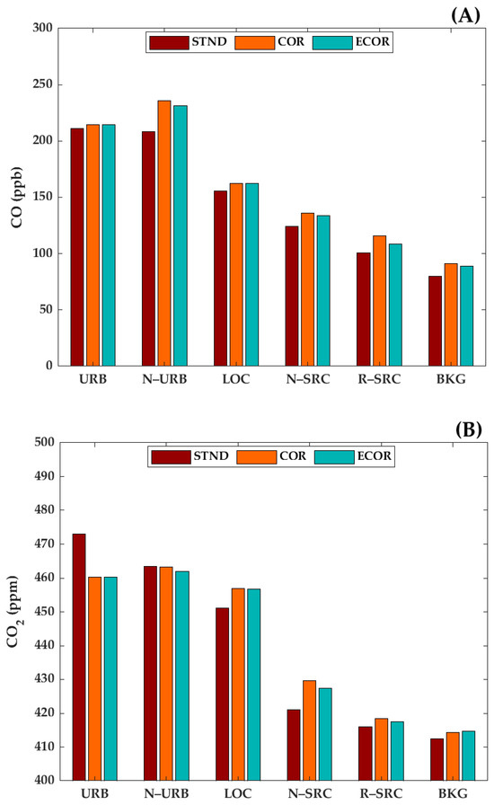
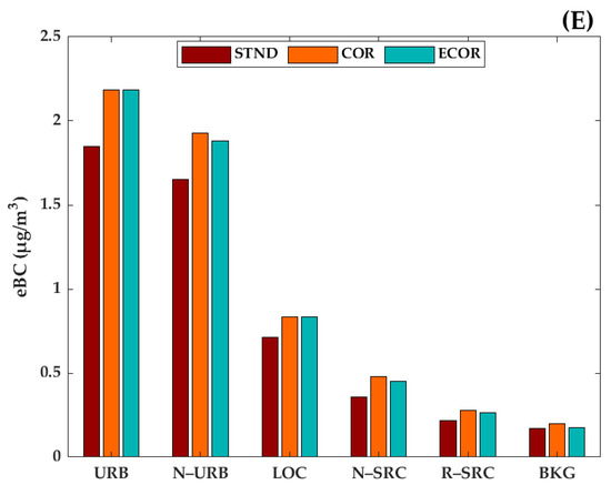
Figure 2.
Concentrations of (A) CO (ppb), (B) CO2 (ppm), (C) CH4 (ppb), (D) SO2 (ppb), and (E) eBC (μg/m3), during the study period, based on standard (STND), corrected (COR), and enhanced corrected (ECOR) categories.
These concentrations, and their variability, are shown in detail in Table 4 (for STND categories), Table 5 (COR), and Table 6 (ECOR).
Table 4.
Concentrations of CO, CO2, CH4, SO2, and eBC during the study period, divided by standard (STND) category, with their respective standard deviation interval (±1σ). A standard deviation of 0.0 indicates a value lower than 0.1, or a very low number of measurements. The URB category has only three measurements.
Table 5.
Concentrations of CO, CO2, CH4, SO2, and eBC during the study period, divided by corrected (COR) category, with their respective standard deviation interval (±1σ). A standard deviation of 0.0 indicates a value lower than 0.1, or a very low number of measurements. The URBcor category has only one measurement.
Table 6.
Concentrations of CO, CO2, CH4, SO2, and eBC during the study period, divided by enhanced corrected (ECOR) category, with their respective standard deviation interval (±1σ). A standard deviation of 0.0 indicates a value lower than 0.1, or a very low number of measurements. The URBecor category has only one measurement.
In addition to categories, the study period needs to be assessed based on the effects of LD on emissions and the balance of local and remote sources. Figure 3 shows, for standard categories (STND), changes in concentrations observed throughout the period. For STND, detailed concentrations and their variability throughout the study period are reported in detail in Table S1A (ALD), S1B (LD), and S1C (PLD). The results are also reported for COR categories in Table S1D (ALD), S1E (LD), and S1F (PLD). For the ECOR categories, the results are shown in Table S1G (ALD), S1H (LD), and S1I (PLD).
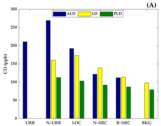
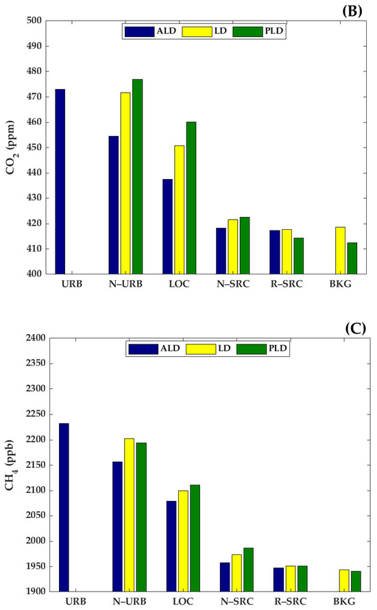
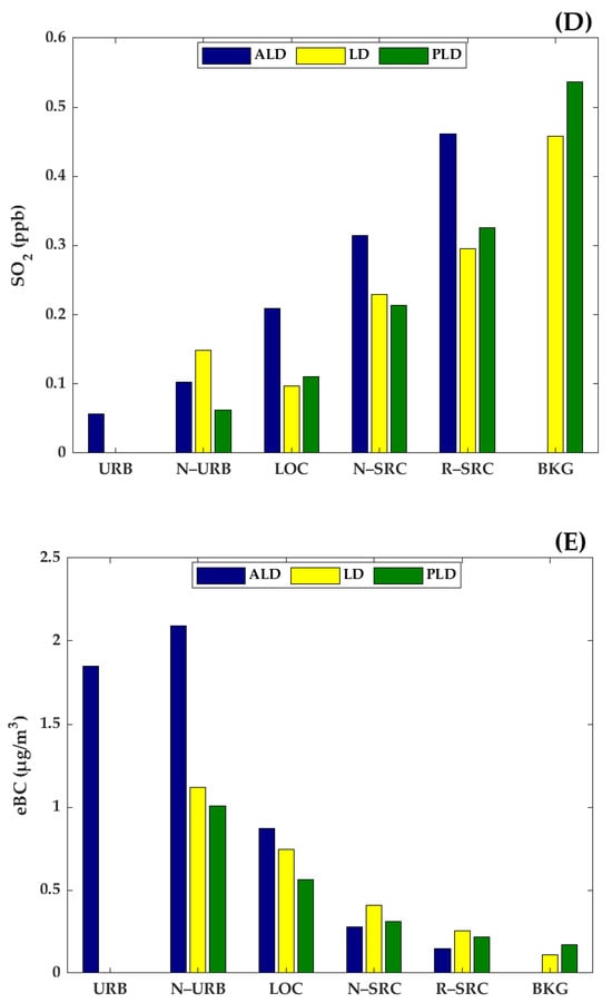
Figure 3.
Variability in the concentration of (A) CO (ppb), (B) CO2 (ppm), (C) CH4 (ppb), (D) SO2 (ppb), and (E) eBC (μg/m3), based on standard categories and divided by period (ALD, LD, and PLD).
From the figures and tables, it is possible to infer that the transition between periods has caused major shifts in the O3/NOx ratio, as a number of categories completely lack coverage under specific circumstances.
3.3. Analysis of Weekly Cycles and Day–Night Contrasts
The assessment of weekly cycles is used in research to discriminate between natural and anthropogenic sources of emission, as the latter can be influenced by a weekly cycle, e.g., higher concentrations of pollutants during weekdays, from Monday (MON) to Friday (FRI), compared to weekends, Saturday (SAT) and Sunday (SUN) [205].
Prior to the implementation of the Kruskal–Wallis [201] and Mann–Whitney U (or Wilcoxon) [202] methodologies, all parameters have been tested for normality using the Shapiro–Wilk [199] and Jarque–Bera [200] tests in R. All tests yielded statistically very significant results (p-value < 0.001), indicating that no parameter follows a normal distribution.
In Figure 4, weekly cycles are reported based on the same format used in previous research [85], now accounting for the three periods. The figure also shows the results of Wilcoxon [202] pairwise tests. The Wilcoxon method compares the concentrations of all evaluated parameters based on a categorization process, creating subsets of the main data record based on periods (ALD, LD, and PLD) and days of the week (weekday, WD, from Monday to Friday, and weekend, WE, from Saturday to Sunday). The resulting pairs are compared to verify the significance of the differences between WD/WE pairs in each period. In Table S2A (STND), B (COR), and C (ECOR), results of the Kruskal–Wallis analysis on weekly cycles are reported. Due to the characteristics of the methodology, a number of gaps are present: these indicate a complete lack of measurements falling under specific hours, or the absence of a sufficient number of pairs for the comparison to be evaluated.
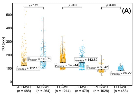
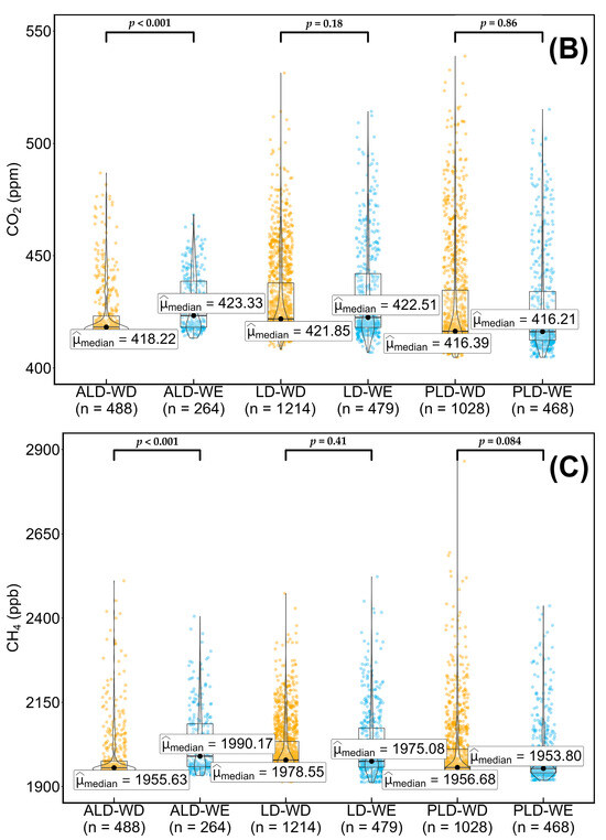
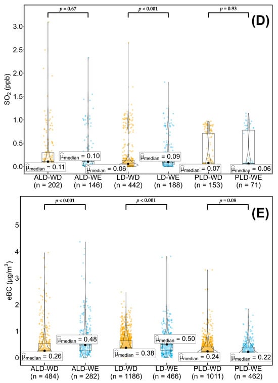
Figure 4.
Weekly cycle of (A) CO (ppb), (B) CO2 (ppm), (C) CH4 (ppb), (D) SO2 (ppb), and (E) eBC (μg/m3), showing the median of each group and the overall distribution of data during the study period. The values on top refer to the p-values of Wilcoxon [202] correlations between specific pairs, assessing the statistical significance of differences between two elements in a pair; values lower than 0.05 indicate relevant differences.
Day–night contrasts at LMT have also been impacted by the COVID-19 LD, as evidenced in previous research [83]. In this work, these contrasts are evaluated using the same methodologies applied to the weekly cycle: the periods are identical (ALD, LD, PLD); however, weekdays and weekends are replaced by day and night, i.e., measurements falling in specific time windows. Hourly measurements have been differentiated between diurnal (DAY, 07:00–18:00 UTC) and nocturnal (NIGHT, 19:00–06:00 UTC), and the results are shown in Figure 5. Table S2D (STND), E (COR), and F (ECOR) report the results of the statistical analyses based on the Kruskal–Wallis [201] test. Due to the characteristics of the methodology and the distribution of measurements, a number of categories could not be assessed.
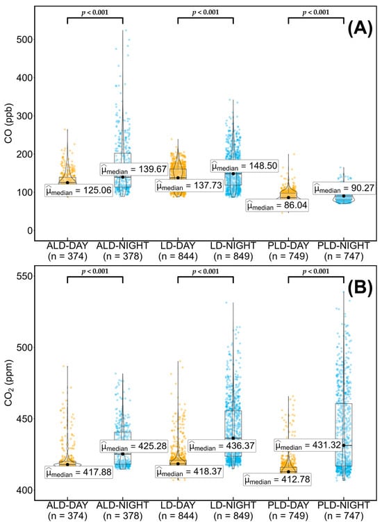
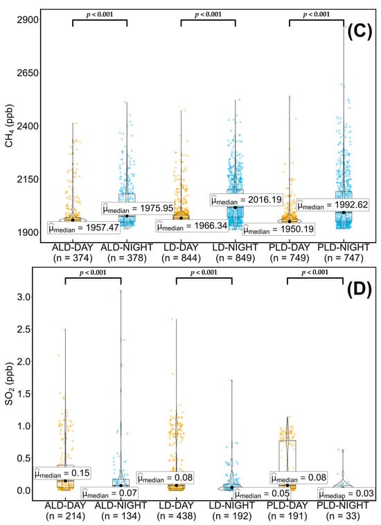
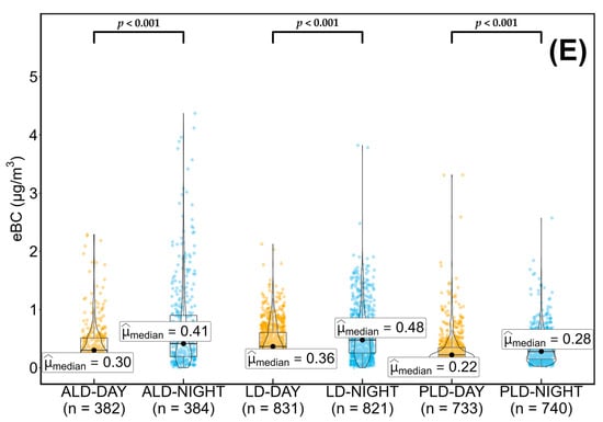
Figure 5.
Day–night contrasts of (A) CO (ppb), (B) CO2 (ppm), (C) CH4 (ppb), (D) SO2 (ppb), and (E) eBC (μg/m3), showing the median of each group and the overall distribution of data during the study period. The values on top refer to the p-values of Wilcoxon [202] correlations between specific pairs, assessing the statistical significance of differences between two elements in a pair; values lower than 0.05 indicate relevant differences.
3.4. Variability of Proximity Progression Factor
The final evaluation of this study is aimed at the Proximity Progression Factor (PPF), introduced in previous research to analyze the progression from local concentrations, enriched in pollutants and other outputs of anthropogenic emissions, from remote sources and the atmospheric background, yielding considerably lower concentrations.
The method was introduced to further highlight the anomaly of SO2 at LMT, as it is the only known parameter yielding a negative PPF, while all other parameters have positive values [192]. A negative PPF indicates remote sources of emission exceeding local ones in terms of concentrations. In this work, the PPF is used for the first time to differentiate between the balances of local-to-remote sources before, during, and after the first 2020 lockdown, and the results are shown in Table 7.
Table 7.
Proximity Progression Factor (PPF), and respective corrections (PPFc, PPFec), evaluating all parameters during the ALD, LD, and PLD periods. “Total” refers to the entire study period.
4. Discussion
The first COVID-19 lockdown (LD) in 2020 constitutes a unique circumstance for the assessment and evaluation of emission sources, thanks to the exploitation of a period characterized by very low anthropogenic emissions. At the Lamezia Terme (LMT) site in Calabria, Italy (Figure 1), previous research analyzed the behavior of a number of parameters at the site [83]. This allowed us to verify a number of hypotheses raised in previous works concerning the contributions of local sources of emission [84,86,119]. However, without an adequate methodology for the assessment of local and remote sources of emission, the previous work accounted for all measurements and therefore could not provide a high degree of detail concerning local variability. Additionally, the previous work did not consider SO2.
The full extent of governmental limitations on anthropic activities in the area around LMT is difficult to assess in detail due to the absence of publicly available data. In a previous work, thanks to data provided by ANAS (the national agency managing highways and state highways), LMT measurements were compared with highway and state highway traffic data in the western Catanzaro isthmus, showing a sharp decline in emissions linked to vehicular traffic in LMT’s northeastern sector [85]. Conversely, waste treatment plants in the industrial area of Lamezia Terme showed no tangible activity reduction due to waste management activities being largely unaffected by governmental restrictions. LMT is located in the northernmost part of the industrial area (Figure 1C), and local near-surface wind circulation is primarily oriented on a W-NE axis, thus making southern winds coming from the industrial area a rare occurrence at LMT [115,116,117].
This work constitutes the first implementation of the ONRPI (Ozone to Nitrogen Oxides Ratio Proximity Indicator) methodology to data gathered during a period with reduced anthropogenic emissions. At the LMT site, the ONRPI has been successfully applied to CO, CO2, and CH4 [87], as well as SO2 and eBC [192], and also allowed the pinpointing of data particularly affected by anthropogenic emissions [190]. This evaluation considers surface data gathered at LMT only, which cannot provide a full regional-scale picture of the balance between emissions during the study period. Previous research based on the ONRPI at LMT shows that the method is very sensitive to short-range emissions [87], especially when very low O3/NOx ratios are considered, where proximity categories can change substantially in the range of only a few kilometers [190].
Despite the effectiveness of the method, in order to be applicable, the ONRPI requires several instruments to operate at the same time: in addition to valid O3 and NOx measurements necessary to calculate the ratio, other instruments or even combinations of instruments all need to operate at the same time to ensure the applicability of the method [87]. Before, during, and after the LD period at LMT, the resulting coverage rate of the ONRPI is affected by these restrictions (Table 1). Overall, the resulting coverage rates fall between the 89.07% and 91.14% thresholds, with a peak of 99.88% during the LD period for SO2. The resulting filtered datasets therefore allowed a detailed analysis of the ALD, LD, and PLD periods at the site. Furthermore, based on the findings of a previous work [190], the correction accounting for NO2 overestimation (COR) and enhanced correction accounting for O3 photochemical production (ECOR) have been extended to all categories from URB to BKG, as they were previously limited to R–SRC and BKG, only, as representative of aged air masses [84,87]. The present work therefore accounts for a total of 18 categories (Table 2), thus marking the most extensive use of the thresholds based on the O3/NOx ratio in research. The analysis of all parameters and their respective variability between ALD, LD and PLD (Figures S1 and S2) is well representative of the characteristics of each parameter and its seasonal shifts. The implementation of proximity categories allows us to better differentiate measurements based on air mass aging indicators, thus leading to a more detailed understanding of local-to-remote balances in the region during the ALD, LD, and PLD periods. CO (Figures S1A and S2A) shows very high peaks in N–URB (269.32 ± 108.7 ppb) and URB (211.29 ± 2.8 ppb) during ALD, with a consequent decline during the LD period (N–URB: 160.53 ± 34.4 ppb) and, consequently, PLD (N–URB: 112.84 ± 13.8 ppb). It is worth mentioning that URB is severely underrepresented in the study period (only three hourly measurements are flagged as URB, thus constituting ~0.06% of the entire dataset, and only one measurement is flagged as URBcor/URBecor), and reported concentrations, as well as the standard deviation, may not reflect pure “urban” conditions at the site. This tendency underlines a major shift in urban-level emissions from high CO outputs attributed to transportation and, most likely, domestic heating, to lower concentrations reflecting reduced emissions at a local scale. LOC and, to some degree, N–SRC show a different behavior, as they reach a peak during the LD period (LOC: 173.76 ± 44.6 ppb; N–SRC: 139.38 ± 28.1 ppb), followed by a gradual decline. This pattern is compatible with CO outputs from domestic heating over a regional area [119], culminating during the LD and entering a decreasing trend due to the increase in temperatures typical of the boreal Spring and the transition to Summer. This particular pattern is barely noticeable in R–SRC, further indicating that its nature could be regional; conversely, BKG shows no clear pattern and is completely absent during the ALD period and most of the LD (98.15 ± 5.0 ppb), with minimal oscillations around concentrations typical of the atmospheric background [87,138]. This is consistent with previous research indicating that the BKG category is characterized by very low variability: it yields the lowest concentrations in the record, and data have minimal oscillations around the average (Figure S2, Table S1).
The influence of domestic heating on LMT’s measurements has been discussed in previous research [84,86,87,119]; however, there are no available data on the true extent of biomass burning related to this particular source of emission. The official air quality report issued by the Regional Council acknowledges the presence of diffused, domestic-related CO emissions contributing up to ~10% of the regional anthropogenic budget, and promotes the implementation of more energy efficient and sustainable means to generate heat in Calabrian households [206]. A study by Putaud et al. [207] found evidence of increased LD emissions in Italy attributable to wood burning for domestic heating purposes.
The previous work on the LD period at LMT found that CO variability was anticorrelated with average temperatures, providing evidence of a temperature-dependent source compatible with domestic heating. Additionally, the hydroxyl radical (OH)—which is an effective sink of CO—is lower during the winter season, thus causing wintertime (in this case, PLD and LD) concentrations of CO to be higher [158,208].
CO2 (Figures S1B and S2B) is characterized by major fluctuations between URB, N–URB, and LOC, with LOC showing a considerable amplitude in these oscillations, as well as the presence of relevant peaks during LD (450.79 ± 19.77 ppm) and PLD (460.11 ± 25.10 ppm) which are not present in the ALD (437.39 ± 11.15 ppm) period. The high degree of oscillations during the LD and, in particular, the PLD periods in N–URB through N–SRC is consistent with photosynthesis and the carbon sink typical of boreal warm seasons: the ONRPI categorizes air masses based on the O3/NOx ratio, and does not therefore consider the photosynthetic sink [87]. The presence of LD and PLD peaks can be observed in N–SRC, while R–SRC and BKG indicate higher degrees of stability and values well representative of atmospheric background levels. During the LD, BKG is 418.59 ± 2.50 ppm, higher than its PLD equivalent (412.38 ± 3.49 ppm) which is affected by photosynthesis. This shows the importance of implementing the ONRPI to factor out the atmospheric background from evaluations on local budgets. A study by Rugano and Caro [209] showed that central Calabria, likely due to its leading rural nature, did not experience the same CO2 reduction seen in northern Italian regions, which were the most affected by LD measures and restrictions. These factors, combined, may explain CO2’s oscillations at the site during the study period.
A peculiar behavior is seen in CH4 (Figures S1C and S2C), where LOC, during the ALD period, is characterized by several peaks, unlike CO2. Although R–SRC and BKG remained stable and showed minimal influence of the LD (LD BKG: 1943.13 ± 7.2 ppb; PLD BKG: 1943.13 ± 7.2 ppb), N–SRC underlines gradual increases during the LD (1973.22 ± 33.7 ppb) and PLD (1986.88 ± 74.4 ppb) periods, which do not match the known patterns of CH4 at the LMT site [86,87,119] and other Mediterranean stations [210,211,212], as the peaks are regularly linked to the Winter season. Other studies in the Mediterranean also reported that CH4 followed patterns not perfectly aligned with the decline in anthropic activities [213]. These patterns show the presence of constant emission sources in the area, which remained rather unaffected by the transition from ALD to LD: this hypothesis is compatible with livestock farming and agricultural activities, mentioned in previous works as possible drivers of local peaks of CH4 [84,87]. The LD increase observed for N–SRC (ALD: 1957.40 ± 32.8 ppb; LD: 1973.22 ± 33.7 ppb; PLD: 1986.88 ± 74.4 ppb), which is in contrast with the known seasonal pattern at LMT, would be compatible with an increase in CH4 mole fractions caused by domestic heating. Waste outputs of CH4 are also expected to remain constant during the LD [214], and an increase in CH4’s atmospheric lifetime caused by reduced NOx outputs has also been considered as a driver of its patterns during the LD and PLD periods [215].
Of particular importance is the behavior of SO2 (Figures S1D and S2D), which contributes to a more detailed understanding of its variability at LMT. While the URB, N–URB, and LOC concentrations are stable during the entire period, the other categories show the presence of remote emission sources affecting SO2 variability at the site. This finding is not in agreement with research on LD variability performed at other sites, where the LD was reported to cause reductions of ~50% in SO2 concentrations [216,217]. There are also reports of areas in Italy where SO2 concentrations were not substantially affected by LD measures, however [69]. At LMT, previous works mentioned the Aeolian Arc of volcanoes, located only a few dozen kilometers from LMT, and maritime shipping as the possible sources of SO2 peaks [163,192]. Eruptions of a significant magnitude are rare and the resulting columns of volcanic outputs would require ad hoc methodologies in order to be assessed in terms of air mass transport and diffusion, such as the upgraded 3D-PSCF model by Dimitriou et al. [218]; however, previous research highlighted the impact of continuous SO2 emissions in the area (e.g., fumaroles, degassing), which have been documented to compromise air quality and worsen health issues in the Aeolian Islands [219,220]. Stromboli alone is known to release ~5 kg of SO2 per second [221]. These continuous emissions are not negligible and affect the regional budget in the western sector of LMT.
The variability of eBC (Figures S1E and S2E) is very closely related to that of CO, with R–SRC and BKG yielding very stable concentrations, while URB to N–SRC are characterized by more fluctuations; in particular, N–URB and LOC show an important local contribution during the ALD period which is not present in N–SRC, underlining the impact of local sources of emission, such as highways, during the ALD period, and the greater impact of domestic heating during the LD period itself, with a number of fluctuations linked by previous research to domestic heating as they were found to be related with the lowest temperature of the period [83]. The change in the amplitude of these fluctuations between the ALD and LD periods in N–SRC is compatible with a greater regional output during the LD period caused by more people relying on domestic heating due to the restrictions introduced by the government [62,64]. It is also worth noting that eBC peaks at ~6.1 μg m3 in the entire dataset, well below the ~9 μg m3 threshold past which MAAP measurements are less reliable [222].
The variability of parameters between periods and proximity categories is also affected by changes in the O3/NOx ratio itself during the study period (Table 3), which are also well representative of shifts in the balance of emissions. From the analysis of categories alone it is possible to infer that the ALD period shows a limited number of hourly data falling under the URB category (STND: 0.33%; COR/ECOR: 0.11%), indicating very high degrees of anthropogenic pollution; additionally, the ALD period is characterized by the absence of measurements falling under the standard BKG category, thus indicating a large-scale influence of anthropogenic emissions before the LD. During the ALD, the atmospheric background is reported only via the implementation of COR and ECOR, which report only 6.64% of measurements falling under this category. During the LD and PLD periods, URB effectively disappears under all circumstances, further showing the shift in anthropogenic emissions occurred during the study period. N–URB also shows a sharp decline but does not completely disappear during the LD and PLD periods. During the PLD period, the BKG categories all reach notable peaks: this is particularly significant in the case of BKGecor at 29.27%, considering that ECOR reduces the O3/NOx ratio by halving O3 under specific circumstances [87]. The intermediate categories show heterogeneous patterns between periods; however, it is worth mentioning the peaks reached by N–SRC during the LD period (up to 55.86% in the case of N–SRCecor), which clearly indicate a strong footprint of anthropogenic emissions over a regional scale unlike the ALD and PLD periods.
In previous research, the analysis of concentrations representative of each category was found to be particularly relevant when applying the ONRPI methodology [84,87,190,192]. In Figure 2, the transition between STND, COR, and ECOR categories shows that STND generally yields lower concentrations, although several exceptions are reported. COR tends to increase the O3/NOx ratio by halving NO2, thus causing more data to fall under BKG and other categories linked to higher ratios. ECOR counterbalances the effect by reducing O3 under specific circumstances, thus impacting R–SRC and BKG. Without considering the anomalous behavior of SO2 (Figure 2D), all other parameters show a clear transition from high URB and N–URB concentrations to very low BKG concentrations. CO (Figure 2A) in particular shows higher N–URB concentrations compared to URB, but it is worth noting that only a fraction of measurements in the ALD period fall under URB, thus affecting its representativeness. The reduced coverage of URB also affects the variability indicator of the category in Table 4, Table 5 and Table 6, as the low number of measurements results in URB concentrations frequently yielding a 1σ interval of ±0.0. Overall, the data show a gradual decrease from URB to BKG, with the well-known exception of SO2, and also show generally decreasing 1σ intervals, thus reflecting high variability around URB, and very low variability around the BKG values, which are very stable.
When the periods are considered instead (Figure 3) (Table S1A–I), the effects of LD restrictions become noticeable: URB is notably absent in LD and PLD, while BKG is not present during the ALD period. Figure 3 shows that even during a period characterized by exceptionally low anthropogenic emissions, the ONRPI is still effective at differentiating data based on the aging of air masses.
The analysis of weekly cycles is an efficient tool to discriminate between natural and anthropogenic sources due to the absence of weekly patterns in the former. It is possible, however, for anthropogenic emissions to have no well-defined weekly patterns, thus restricting this method to specific circumstances. At LMT, the analysis of weekly patterns has improved over time [85,86,87,119,163,184,190] and presently constitutes the most detailed evaluation of this kind currently being performed in the national network of atmospheric stations. As previous research showed non-negligible weekly patterns, the study period was assessed to verify the statistical significance of the differences between WD (weekday, MON-FRI) and WE (weekend, SAT-SUN). Figure 4 shows, in addition to the medians of all distributions falling in each combination of period and WD/WE, the results of pairwise Wilcoxon (Mann–Whitney U) [202] tests. For CO (Figure 4A), the results show the presence of well-defined weekly patterns in ALD (WDμ: 122.13 ppb; WEμ: 149.71 ppb; p-value < 0.001) and PLD (WDμ: 143.44 ppb; WEμ: 143.82 ppb; p-value = 0.41), compatible with regular anthropic activities characterized by such cycles (e.g., transportation), and the absence of similar patterns during the LD period, as most CO outputs were likely resulting from domestic heating and remained constant over time. The observed change in behavior occurred in a very short time span and is representative of the shifts in emission balances that occurred between the ALD and LD periods. CO2 (Figure 4B) shows a very significant weekly pattern during the ALD period (WDμ: 418.22 ppm; WEμ: 423.33 ppm; p-value < 0.001), and non-significant patterns during LD (p-value = 0.18) and PLD (p-value = 0.86): while the former is deemed a direct consequence of governmental restrictions, the latter yields lower concentrations, typical of the warm boreal season due to intense photosynthetic activity [87,119,138,190] and the presence of anthropic activities not influenced by a proper weekly cycle, such as summertime tourism in Calabria [85]. CH4 (Figure 4C) shows an identical pattern, with a very significant ALD (WDμ: 1955.63 ppb; WEμ: 1990.17 ppb; p-value < 0.001) weekly cycle and the absence of such patterns during the LD and PLD. Like CO2, CH4 concentrations during the warm seasons have been reported to be considerably lower at LMT [86,87,119,138]. With constant emission sources such as livestock reported around the site [84,87], the absence of a weekly pattern becomes prominent in the PLD (WDμ: 1956.68 ppb; WEμ: 1953.80 ppb; p-value = 0.084) period in particular, with domestic heating no longer being a factor due to the higher temperatures of the period. Waste treatment-related emissions are also believed to be largely unaffected by the LD. Conversely, these extra emissions would be the cause of very significant weekly cycles during the ALD; the consequent LD would then distribute these emissions equally during the week, thus causing an abrupt transition from an extremely significant (ALD, p < 0.001) to a non-significant (LD, p = 0.41) cycle. The weekly cycle of SO2 (Figure 4D) shows an “anomaly within the anomaly”, as the LD period is the only one characterized by a significant weekly cycle (WDμ: 0.06 ppb; WEμ: 0.09 ppb; p-value < 0.001), with WE concentrations ~50% higher than their WD counterparts. The significance of this pattern could be due to the very low concentrations reported at LMT during the study period, and needs to be assessed in greater detail using proximity categories. Furthermore, SO2 variability is influenced by sources such as maritime shipping in the Mediterranean, which are difficult to factor out [138]. eBC (Figure 4E) shows significant ALD (WDμ: 0.26 μg/m3; WEμ: 0.48 μg/m3; p-value < 0.001) and LD (WDμ: 0.38 μg/m3; WEμ: 0.50 μg/m3; p-value < 0.001) weekly cycles likely driven by domestic heating, as the difference between WD and WE is considerably lower in the LD period (0.12 μg/m3) compared to the ALD period (0.22 μg/m3). This does not explain, however, the presence of a significant cycle during the LD, which is absent in CO. Conversely, the PLD is characterized by lower concentrations typical of warm seasons which make weekly cycles of eBC less prominent, as previously evidenced in another work, where eBC variability at the site is generally driven by sporadic, open fire-related outputs [119]. In addition to the total concentrations, this study performed a detailed weekly cycle analysis accounting for all categories, i.e., STND (Table S2A), COR (Table S2B), and ECOR (Table S2C). The Kruskal–Wallis [201] test requires a sufficient number of measurements in each WD/WE pair to be performed, thus leading to gaps. Specifically, none of the URB cycles could be assessed, and many N–URB and BKG were also affected due to the absence of data and the effects of correction factors. Overall, the intermediate category N–SRC shows to be the most affected by weekly cycles, reflecting weekly changes in the balance of emissions on a local-to-regional scale, while N–URB, LOC and R–SRC are less affected, indicating that sources in the area of LMT, as well as remote sources, are more dispersed. BKG is even less affected, showing that the atmospheric background remained stable during the period, and the ONRPI methodology can effectively differentiate it from other sources. When it comes to specific parameters, CO and eBC show the presence of the highest number of significant weekly cycles, with CO characterizing the ALD and PLD periods, indicating a strong fingerprint related to emissions that were affected by governmental restrictions, and eBC the LD period. SO2 and eBC yield no valid weekly cycles during the PLD period, thus showing evidence of a shift in the prevailing nature and behavior of emissions [119,163,192]. A study by Grivas et al. [223] showed a significant BC rebound in Athens, Greece following the 2020 LD; at LMT, a PLD rebound of eBC is reported for categories up until N–SRC, while R–SRC and BKG remain unaffected (Figures S1E and S2E). The absence of a weekly cycle does not automatically exclude anthropic influences; instead, it indicates a shift towards emissions more evenly distributed over the course of a week, with no substantial differences between WD and WE.
The analysis of contrasts between day and night, which are known to characterize the variability of data at LMT [83,85,86,87,184,190], is assessed in this work using the same methodology applied to the weekly cycle [85]. Previous research evaluated these contrasts and reported on their variability without implementing the same statistical methods applied to the weekly cycle; in this work, the two assessments are homogenized, thus showing a new and integrated method for the analysis of the day–night contrast at LMT. The pairwise Wilcoxon [202] test applied to diurnal/nocturnal pairs shows statistically relevant results for all combinations (Figure 5), indicating that the contrast is a key regulator of local variability, unlike the weekly cycle. Like the weekly cycle, this is also affected by the coverage of specific categories, and several gaps (most notably, the entire URB category) are present (Table S2D–F). From the statistical analysis, the intermediate categories LOC and N–SRC are the most affected, well representing the effects of diurnal/nocturnal shifts in emission on a local-to-regional scale. As a parameter, CO2 is considerably affected by daily oscillations due to increased photosynthesis linked to the boreal Summer in PLD [119], although the ALD and LD are also partially affected by the phenomenon, as previously reported in Figures S1B and S2B. Conversely, SO2 is the least affected, showing that remote sources (volcanoes, maritime shipping) [163] not influenced by the day–night contrasts are prominent regulators of its variability. It is also worth mentioning that CO yields relevant day–night contrasts throughout the entire period, while eBC (which has so far shown a very similar behavior) does so only during the PLD.
The last evaluation of the study relies on the PPF, introduced in a previous work [192], to assess the balance between local and remote sources during the study period. The PPF indicates whether a given parameter follows a regular pattern from local, enriched concentrations attributable to anthropogenic emissions, and remote, very low concentrations representative of the atmospheric background. In previous research, all parameters with the exception of SO2 yielded positive PPF values, highlighting the anomaly of SO2 at the site and showing the presence of remote sources exceeding local outputs. In Table 7, PPF values of ALD, LD, and PLD, and their corrected counterparts (PPFc, PPFec), are reported and compared to the cumulative study period. During the ALD period, PPF and PPFec values could not be computed due to the absence of BKG measurements. The results show a strong negative tendency for SO2, with the exception of ALD, where the PPFc yields −0.046, thus indicating a virtually “neutral” scenario with respect to proximity categories. eBC yields very high values, especially during the ALD, with a PPFc of 0.527 indicating a remarkable difference between local and remote sources, likely the effect of the peaks in anthropic activities during the boreal Winter that preceded the LD, during which eBC’s PPF reaches the non-negligible value of 0.42. CO2 and CH4 show a stable behavior, indicating for CH4 the presence of local/constant emission sources in the area, as hypothesized in previous research [84,86,87]. CO’s PPFc peaks during the LD at 0.169 and shows lower values during the PLD compared to the other periods; this indicates an overall reduction in concentrations, with local sources of emission being close to the atmospheric background. The difference in the balance of CO and eBC shows that the latter is more influenced by local sources of emissions; while this can be caused by the considerably lower atmospheric lifetime of BC [182] compared to CO [142], the findings of this study suggest that local CO-BC balances need further investigation. Overall, the first implementation of the PPF in a scenario such as the COVID-19 LD of 2020 has allowed the changes in local-to-remote emission sources to be highlighted, with heterogeneous results due to the characteristics of each parameter.
In terms of future perspectives, LMT is part of a consortium of four atmospheric observatories in the country implementing stable carbon isotope measurements of CO2 (δ13C-CO2) and CH4 (δ13C-CH4) [56]. Although these measurements were not in place at the time of the 2020 LD, a more accurate understanding of LMT’s CO2 and CH4 variability would allow researchers, to a certain degree, to retroactively test the hypotheses made in this study and verify them in the scope of source apportionment.
5. Conclusions
At the Lamezia Terme (LMT) WMO/GAW observation site in Calabria, Southern Italy, the ONRPI (Ozone to Nitrogen Oxides Ratio Proximity Indicator) has been applied to data measured between February and July 2020 to assess the variability of local and remote sources of emission of CO, CO2, CH4, SO2, and eBC. Based on the findings of previous works, the ONRPI has been expanded with a total of 18 categories, accounting for two distinct correction factors (COR and ECOR) in addition to the standard (STND) methodology. The present framework constitutes the most complete use of this methodology in the field.
The analysis of tendencies observed between ALD (ante-lockdown), LD (lockdown), and PLD (post-lockdown) periods has allowed us to discriminate between local and remote sources, with SO2 showing a notable anomaly, i.e., the presence of remote sources exceeding their local counterparts. In the transition from ALD to PLD, air mass aging indicators show a gradual increase in the O3/NOx ratio, with data heavily affected by anthropogenic emissions being limited to the ALD period only, and data representative of the atmospheric background being more common in the PLD.
A detailed weekly cycle analysis was performed to assess the influence of anthropic activities in a period characterized by governmental restrictions and highlighted prominent patterns in CO and eBC, as well as regional-scale shifts in these cycles which were not observed at local scales. The analysis of day–night contrasts, i.e., the difference between diurnal and nocturnal measurements, was evaluated in this study with additional statistical methods compared to previous research on LMT data and showed a higher significance rate compared to the weekly cycle.
The implementation of the Proximity Progression Factor (PPF) has also allowed us to improve the characterization and understanding of local-to-remote balances at LMT, especially for CO. SO2 showed the same anomalies reported in previous studies; however, during the LD a “neutral” behavior emerged. CO2 and CH4 showed a stable pattern, compatible in the case of CH4 with local/constant sources of emission (e.g., livestock farming) hypothesized in previous research and relatively unaffected by the LD. Overall, the study shows the potential of the ONRPI methodology as an effective tool in source apportionment even in exceptional circumstances, such as the COVID-19 LD and the consequent reduction in anthropic activities caused by governmental policies and regulations.
Supplementary Materials
The following supporting information can be downloaded at https://www.mdpi.com/article/10.3390/pollutants6010019/s1, Figure S1A–E: Concentrations of evaluated parameters (CO, CO2, CH4, SO2, eBC) differentiated by proximity category and period; Figure S2A–E: Alternate versions of S1 using boxplots; Table S1A–I: Concentrations of all parameters divided by period and proximity category, also accounting for the COR and ECOR corrections; Table S2A–F: Statistical analysis applied to weekly cycles and day–night contrasts.
Author Contributions
Conceptualization, F.D.; methodology, F.D.; software, F.D., D.G., T.L.F. and M.B.; validation, D.G., I.A. and M.B.; formal analysis, F.D.; investigation, F.D.; resources, C.R.C.; data curation, D.G., I.A. and M.B.; writing—original draft preparation, F.D. and T.L.F.; writing—review and editing, F.D., D.G., I.A., T.L.F., M.B. and C.R.C.; visualization, F.D. and T.L.F.; supervision, C.R.C.; project administration, C.R.C.; funding acquisition, C.R.C. All authors have read and agreed to the published version of the manuscript.
Funding
This research was funded by AIR0000032–ITINERIS, the Italian Integrated Environmental Research Infrastructures System (D.D. n. 130/2022-CUP B53C22002150006) under the EU—Next Generation EU PNRR—Mission 4 “Education and Research”—Component 2: “From research to business”—Investment 3.1: “Fund for the realization of an integrated system of research and innovation infrastructures”.
Data Availability Statement
The data are not presently available as they are subject to other ongoing research.
Acknowledgments
The authors would like to acknowledge the contribution of the three anonymous reviewers who helped expand and improve this manuscript.
Conflicts of Interest
The authors declare no conflicts of interest.
References
- Holland, M.R. Assessment of the economic costs of damage caused by air-pollution. Water Air Soil Pollut. 1995, 85, 2583–2588. [Google Scholar] [CrossRef]
- Lelieveld, J.; Evans, J.; Fnais, M.; Giannadaki, D.; Pozzer, A. The contribution of outdoor air pollution sources to premature mortality on a global scale. Nature 2015, 525, 367–371. [Google Scholar] [CrossRef]
- Pinakana, S.D.; Robles, E.; Mendez, E.; Raysoni, A.U. Assessment of Air Pollution Levels during Sugarcane Stubble Burning Event in La Feria, South Texas, USA. Pollutants 2023, 3, 197–219. [Google Scholar] [CrossRef]
- Liu, Q.; Liu, Y. Measuring Biogenic Volatile Organic Compounds from Leaves Exposed to Submicron Black Carbon Using Portable Sensor. Pollutants 2024, 4, 187–195. [Google Scholar] [CrossRef]
- Pitiranggon, M.; Johnson, S.; Spira-Cohen, A.; Eisl, H.; Ito, K. Determining Sources of Air Pollution Exposure Inequity in New York City Through Land-Use Regression Modeling of PM2.5 Constituents. Pollutants 2025, 5, 2. [Google Scholar] [CrossRef]
- Orset, C.; Monnier, M. Perceived economic benefits of reducing the risk of mortality from air pollution in France. J. Environ. Assess. Policy Manag. 2025, 27, 2550002. [Google Scholar] [CrossRef]
- Li, Y.; Ye, R.J.; Yang, S.Q.; Yu, H.; Yu, B.Q.; Feng, J.; Yuan, Q. Global, regional, and national burden of neonatal disorders and subtypes attributable to air pollution from 1990 to 2021: A systematic analysis of the Global Burden of Disease Study 2021. J. Health Popul. Nutr. 2025, 44, 157. [Google Scholar] [CrossRef]
- Zhang, Y.; Wang, W.; Dai, K.; Huang, Y.; Wang, R.; He, D.; He, J.; Liang, H. Global lung cancer burden attributable to air fine particulate matter and tobacco smoke exposure: Spatiotemporal patterns, sociodemographic characteristics, and transnational inequalities from 1990 to 2021. BMC Public Health 2025, 25, 1260. [Google Scholar] [CrossRef]
- Prüss-Üstün, A.; Wolf, J.; Corvalán, C.F.; Bos, R.; Neira, M.P. Preventing Disease Through Healthy Environments: A Global Assessment of the Burden of Disease from Environmental Risks; World Health Organization: Geneva, Switzerland, 2016; Available online: https://iris.who.int/handle/10665/204585 (accessed on 13 November 2025).
- Knabe, W. Effects of sulfur dioxide on terrestrial vegetation. Ambio 1976, 5, 213–218. [Google Scholar]
- Likens, G.E. Chemical wastes in our atmosphere–An ecological crisis. Ind. Crisis Q. 1987, 1, 13–33. [Google Scholar] [CrossRef]
- Alexeyev, V.A. Impacts of air pollution on far north forest vegetation. Sci. Total Environ. 1995, 160–161, 605–617. [Google Scholar] [CrossRef]
- Saare, L.; Talkop, R.; Roots, O. Air pollution effects on terrestrial ecosystems in Estonia. Water Air Soil Poll. 2001, 130, 1181–1186. [Google Scholar] [CrossRef]
- Puc, M. Influence of meteorological parameters and air pollution on hourly fluctuation of birch (Betula L.) and ash (Fraxinus L.) airborne pollen. Ann. Agric. Environ. Med. 2012, 19, 660–665. [Google Scholar]
- Yue, X.; Unger, N. Fire air pollution reduces global terrestrial productivity. Nat. Commun. 2018, 9, 5413. [Google Scholar] [CrossRef]
- Barton, M.G.; Henderson, I.; Border, J.A.; Siriwardena, G. A review of the impacts of air pollution on terrestrial birds. Sci. Total Environ. 2023, 873, 162136. [Google Scholar] [CrossRef]
- Ryalls, J.M.W.; Bromfield, L.M.; Mullinger, N.J.; Langford, B.; Mofikoya, A.O.; Pfrang, C.; Nemitz, E.; Blande, J.D.; Girling, R.D. Diesel exhaust and ozone adversely affect pollinators and parasitoids within flying insect communities. Sci. Total Environ. 2025, 958, 177802. [Google Scholar] [CrossRef] [PubMed]
- Bhugwant, C.; Siéja, B.; Bessafi, M.; Staudacher, T.; Ecormier, J. Atmospheric sulfur dioxide measurements during the 2005 and 2007 eruption of the Piton de La Fournaise volcano: Implications for human health and environmental changes. J. Volcanol. Geoth. Res. 2009, 184, 208–224. [Google Scholar] [CrossRef]
- Schmidt, A.; Ostro, B.; Carslaw, K.S.; Wilson, M.; Thordarson, T.; Mann, G.W.; Simmons, A.J. Excess mortality in Europe following a future Laki-style Icelandic eruption. Proc. Natl. Acad. Sci. USA 2011, 108, 15710–15715. [Google Scholar] [CrossRef]
- Viana, M.; Pey, J.; Querol, X.; Alastuey, A.; de Leeuw, F.; Lükewille, A. Natural sources of atmospheric aerosols influencing air quality across Europe. Sci. Total. Environ. 2014, 472, 825–833. [Google Scholar] [CrossRef]
- Kochi, T.; Iwasawa, S.; Nakano, M.; Tsuboi, T.; Tanaka, S.; Kitamura, H.; Wilson, D.J.; Takebayashi, T.; Omae, K. Influence of sulfur dioxide on the respiratory system of Miyakejima adult residents 6 years after returning to the island. J. Occup. Health. 2017, 59, 313–326. [Google Scholar] [CrossRef]
- Sellitto, P.; Zanetel, C.; di Sarra, A.; Salerno, G.; Tapparo, A.; Meloni, D.; Pace, G.; Caltabiano, T.; Briole, P.; Legras, B. The impact of Mount Etna sulfur emissions on the atmospheric composition and aerosol properties in the central Mediterranean: A statistical analysis over the period 2000–2013 based on observations and Lagrangian modelling. Atmos. Environ. 2017, 148, 77–88. [Google Scholar] [CrossRef]
- Opolot, M.; Omara, T.; Adaku, C.; Ntambi, E. Pollution Status, Source Apportionment, Ecological and Human Health Risks of Potentially (Eco)toxic Element-Laden Dusts from Urban Roads, Highways and Pedestrian Bridges in Uganda. Pollutants 2023, 3, 74–88. [Google Scholar] [CrossRef]
- Narayanan, C.; Nazarenko, Y. In Silico Characterization of Molecular Interactions of Aviation-Derived Pollutants with Human Proteins: Implications for Occupational and Public Health. Atmosphere 2025, 16, 919. [Google Scholar] [CrossRef]
- Stefanis, C.; Manisalidis, I.; Stavropoulou, E.; Stavropoulos, A.; Tsigalou, C.; Voidarou, C.; Constantinidis, T.C.; Bezirtzoglou, E. Assessing the Impact of Aviation Emissions on Air Quality at a Regional Greek Airport Using Machine Learning. Toxics 2025, 13, 217. [Google Scholar] [CrossRef]
- Deng, S.; Zhou, S.; Zhang, L.; Zhao, J. Study on Green Airport Construction and Aviation Pollution Control: A Case Study of Four International Airports. Atmosphere 2025, 16, 261. [Google Scholar] [CrossRef]
- Phillips, D. The Potential Health Benefits of Reduced PM2.5 Exposure Through a More Rapid Green Transition of South Korea’s Transport Sector. Pollutants 2025, 5, 35. [Google Scholar] [CrossRef]
- Armenta-Déu, C. Environmental Impact of Urban Surface Transportation: Influence of Driving Mode and Drivers’ Attitudes. Pollutants 2025, 5, 5. [Google Scholar] [CrossRef]
- Maciejewska, M.; Kurzawska-Pietrowicz, P. Towards Sustainable Airport Operations: Emission Analysis of Taxiing Solutions. Sustainability 2025, 17, 8242. [Google Scholar] [CrossRef]
- Bseibsu, A.; Madhuranthakam, C.M.R.; Yetilmezsoy, K.; Almansoori, A.; Elkamel, A. Numerical Simulation of Dispersion Patterns and Air Emissions for Optimal Location of New Industries Accounting for Environmental Risks. Pollutants 2022, 2, 444–461. [Google Scholar] [CrossRef]
- El Ghazi, I.; Berni, I.; Menouni, A.; Amane, M.; Kestemont, M.-P.; El Jaafari, S. Exposure to Air Pollution from Road Traffic and Incidence of Respiratory Diseases in the City of Meknes, Morocco. Pollutants 2022, 2, 306–327. [Google Scholar] [CrossRef]
- Giacosa, G.; Barnett, C.; Rainham, D.G.; Walker, T.R. Characterization of Annual Air Emissions Reported by Pulp and Paper Mills in Atlantic Canada. Pollutants 2022, 2, 135–155. [Google Scholar] [CrossRef]
- Walker, T.R. Effectiveness of the National Pollutant Release Inventory as a Policy Tool to Curb Atmospheric Industrial Emissions in Canada. Pollutants 2022, 2, 289–305. [Google Scholar] [CrossRef]
- Rivera-Cárdenas, C.I.; Arellano, T. The Tula Industrial Area Field Experiment: Quantitative Measurements of Formaldehyde, Sulfur Dioxide, and Nitrogen Dioxide Emissions Using Mobile Differential Optical Absorption Spectroscopy Instruments. Pollutants 2024, 4, 463–473. [Google Scholar] [CrossRef]
- Fugiel, A.; Burchart-Korol, D.; Czaplicka-Kolarz, K.; Smoliński, A. Environmental impact and damage categories caused by air pollution emissions from mining and quarrying sectors of European countries. J. Clean. Prod. 2017, 143, 159–168. [Google Scholar] [CrossRef]
- Ngwu, T.A.; Oramah, C.P.; Somprasong, K.; Charoentanaworakun, C. Evaluating the Cost-Effectiveness of Environmental Protection Plans in Quarrying Using the Social Return on Investment Framework. Pollutants 2025, 5, 42. [Google Scholar] [CrossRef]
- Segerson, K. Air pollution and agriculture: A review and evaluation of policy interactions. In Commodity and Resource Policies in Agricultural Systems; Agricultural Management and Economics; Just, R.E., Bockstael, N., Eds.; Springer: Berlin/Heidelberg, Germany, 1991. [Google Scholar] [CrossRef]
- Aneja, V.P.; Schlesinger, W.H.; Erisman, J.W. Effects of agriculture upon the air quality and climate: Research, policy, and regulations. Environ. Sci. Technol. 2009, 43, 4234–4240. [Google Scholar] [CrossRef]
- Harizanova-Bartos, H.; Stoyanova, Z. Impact of agriculture on air pollution. CBU Int. Conf. Proc. 2018, 6, 1071–1076. [Google Scholar] [CrossRef]
- Sillmann, J.; Aunan, K.; Emberson, L.; Büker, P.; Van Oort, B.; O’Neill, C.; Otero, N.; Pandey, D.; Brisebois, A. Combined impacts of climate and air pollution on human health and agricultural productivity. Environ. Res. Lett. 2021, 16, 093004. [Google Scholar] [CrossRef]
- Baghel, N.; Singh, K.; Lakhani, A.; Kumari, K.M.; Satsangi, A. A Study of Real-Time and Satellite Data of Atmospheric Pollutants during Agricultural Crop Residue Burning at a Downwind Site in the Indo-Gangetic Plain. Pollutants 2023, 3, 166–180. [Google Scholar] [CrossRef]
- Zhao, K.; Tian, X.; Lai, W.; Xu, S. Agricultural production and air pollution: An investigation on crop straw fires. PLoS ONE 2024, 19, e0303830. [Google Scholar] [CrossRef]
- Andersen, I.; Lundqvist, G.R.; Molhave, L. Formaldehyde in the home atmosphere. Proposed introduction of limits for airborne contaminants. Ugeskr. Laeger 1979, 141, 966–971. [Google Scholar] [PubMed]
- Merchán, M.L.; De La Serna, J. Formadehyde as an indoor pollutant. Toxicol. Environ. Chem. 1986, 13, 17–25. [Google Scholar] [CrossRef]
- Schachter, E.N.; Witek, T.J.; Tosun, T.; Leaderer, B.P.; Beck, G.J. A study of respiratory effects from exposure to 2 ppm formaldehyde in healthy subjects. Arch. Environ. Health 1986, 41, 229–239. [Google Scholar] [CrossRef] [PubMed]
- Cao, Z.; Xu, F.; Covaci, A.; Wu, M.; Yu, G.; Wang, B.; Deng, S.; Huang, J. Differences in the seasonal variation of brominated and phosphorus flame retardants in office dust. Environ. Int. 2014, 65, 100–106. [Google Scholar] [CrossRef]
- Kausar, A.; Ahmad, I.; Zhu, T.; Shahzad, H. Impact of Indoor Air Pollution in Pakistan—Causes and Management. Pollutants 2023, 3, 293–319. [Google Scholar] [CrossRef]
- Thunis, P.; Clappier, A.; Tarrason, L.; Cuvelier, C.; Monteiro, A.; Pisoni, E.; Wesseling, J.; Belis, C.A.; Pirovano, G.; Janssen, S.; et al. Source apportionment to support air quality planning: Strengths and weaknesses of existing approaches. Environ. Int. 2019, 130, 104825. [Google Scholar] [CrossRef]
- Liu, H.; Li, B.; Qi, H.; Ma, L.; Xu, J.; Wang, M.; Ma, W.; Tian, C. Source Apportionment and Toxic Potency of Polycyclic Aromatic Hydrocarbons (PAHs) in the Air of Harbin, a Cold City in Northern China. Atmosphere 2021, 12, 297. [Google Scholar] [CrossRef]
- Han, Y.; Wang, Z.; Zhou, J.; Che, H.; Tian, M.; Wang, H.; Shi, G.; Yang, F.; Zhang, S.; Chen, Y. PM2.5-Bound Heavy Metals in Southwestern China: Characterization, Sources, and Health Risks. Atmosphere 2021, 12, 929. [Google Scholar] [CrossRef]
- Coelho, S.; Ferreira, J.; Rodrigues, V.; Lopes, M. Source apportionment of air pollution in European urban areas: Lessons from the ClairCity project. J. Environ. Manage. 2022, 320, 115899. [Google Scholar] [CrossRef]
- Coelho, S.; Ferreira, J.; Lopes, M. Source apportionment of air pollution in urban areas: A review of the most suitable source-oriented models. Air Q. Atmos. Health 2023, 16, 1185–1194. [Google Scholar] [CrossRef]
- Lino, S.; Toscano, D.; Piccoli, A.; Riccio, A.; De Angelis, E.; Pirovano, G.; Agresti, V. Source apportionment of key air pollutants in Naples using a high-resolution WRF-CAMx-PSAT modeling framework. Atmos. Environ. 2026, 364, 121638. [Google Scholar] [CrossRef]
- Brownlow, R.; Lowry, D.; Fisher, R.E.; France, J.L.; Lanoisellé, M.; White, B.; Wooster, M.J.; Zhang, T.; Nisbet, E.G. Isotopic ratios of tropical methane emissions by atmospheric measurement. Glob. Biogeochem. Cycles 2017, 31, 1408–1419. [Google Scholar] [CrossRef]
- Fiehn, A.; Eckl, M.; Kostinek, J.; Gałkowski, M.; Gerbig, C.; Rothe, M.; Röckmann, T.; Menoud, M.; Maazallahi, H.; Schmidt, M.; et al. Source apportionment of methane emissions from the Upper Silesian Coal Basin using isotopic signatures. Atmos. Chem. Phys. 2023, 23, 15749–15765. [Google Scholar] [CrossRef]
- Buono, A.; Zaccardo, I.; D’Amico, F.; Lapenna, E.; Cardellicchio, F.; Laurita, T.; Amodio, D.; Colangelo, C.; Di Fiore, G.; Giunta, A.; et al. Expanding Continuous Carbon Isotope Measurements of CO2 and CH4 in the Italian ICOS Atmospheric Consortium: First Results from the Continental POT Station in Potenza (Basilicata). Atmosphere 2025, 16, 951. [Google Scholar] [CrossRef]
- Al-Shalan, A.; Lowry, D.; Fisher, R.E.; Nisbet, E.G.; Zazzeri, G.; Al-Sarawi, M.; France, J.L. Methane emissions in Kuwait: Plume identification, isotopic characterisation and inventory verification. Atmos. Environ. 2022, 268, 118763. [Google Scholar] [CrossRef]
- Woolley Maisch, C.A.; Fisher, R.E.; France, J.L.; Lowry, D.; Lanoisellé, M.; Röckmann, T.; van der Veen, C.; Nisbet, E.G. Characterising methane emissions from dairy farm sources using mobile and dual-isotope measurements in Jersey, Channel Islands. Atmos. Environ. X 2025, 28, 100384. [Google Scholar] [CrossRef]
- Woolley Maisch, C.A.; France, J.L.; Fisher, R.E.; Lowry, D.; Forster, G.; To, T.H.; Irakulis-Loitxate, I.; Garrard, N.; Nguyen, D.T.C.; Nguyen, T.T.N.; et al. Identification of sources of methane in Ho Chi Minh City, Vietnam. ACS EST Air 2025. [Google Scholar] [CrossRef]
- Kazemi Garajeh, M.; Laneve, G.; Rezaei, H.; Sadeghnejad, M.; Mohamadzadeh, N.; Salmani, B. Monitoring Trends of CO, NO2, SO2, and O3 Pollutants Using Time-Series Sentinel-5 Images Based on Google Earth Engine. Pollutants 2023, 3, 255–279. [Google Scholar] [CrossRef]
- Barrese, E.; Valentini, M.; Scarpelli, M.; Samele, P.; Malacaria, L.; D’Amico, F.; Lo Feudo, T. Assessment of Formaldehyde’s Impact on Indoor Environments and Human Health via the Integration of Satellite Tropospheric Total Columns and Outdoor Ground Sensors. Sustainability 2024, 16, 9669. [Google Scholar] [CrossRef]
- Italian Republic. Decree of the President of the Council of Ministers, 9 March 2020. GU Serie Generale n. 62. Available online: https://www.gazzettaufficiale.it/eli/id/2020/03/09/20A01558/sg (accessed on 4 September 2025).
- Loperte, S. A Trans-Disciplinary and Integral Model of Participatory Planning for a More Sustainable and Resilient Basilicata. Pollutants 2022, 2, 205–233. [Google Scholar] [CrossRef]
- Italian Republic. Decree of the President of the Council of Ministers, 18 May 2020. GU Serie Generale n. 127. Available online: https://www.gazzettaufficiale.it/eli/id/2020/05/18/20A02727/sg (accessed on 4 September 2025).
- Giani, P.; Castruccio, S.; Anav, A.; Howard, D.; Hu, W.; Crippa, P. Short-term and long-term health impacts of air pollution reductions from COVID-19 lockdowns in China and Europe: A modelling study. Lancet Planet. Health 2020, 4, 474–482. [Google Scholar] [CrossRef] [PubMed]
- Baldasano, J. COVID-19 lockdown effects on air quality by NO2 in the cities of Barcelona and Madrid (Spain). Sci. Total Environ. 2020, 741, 140353. [Google Scholar] [CrossRef]
- Menut, L.; Bessagnet, B.; Siour, G.; Mailler, S.; Pennel, R.; Cholakian, A. Impact of lockdown measures to combat Covid-19 on air quality over western Europe. Sci. Total Environ. 2020, 741, 140426. [Google Scholar] [CrossRef]
- Habibi, H.; Awal, R.; Fares, A.; Ghahremannejad, M. COVID-19 and the Improvement of the Global Air Quality: The Bright Side of a Pandemic. Atmosphere 2020, 11, 1279. [Google Scholar] [CrossRef]
- Collivignarelli, M.C.; Abba, A.; Bertanza, G.; Pedrazzani, R.; Ricciardi, P.; Miino, M.C. Lockdown for CoViD-2019 in Milan: What are the effects on air quality? Sci. Total Environ. 2020, 732, 139280. [Google Scholar] [CrossRef]
- Berman, J.D.; Ebisu, K. Changes in US air pollution during the COVID-19 pandemic. Sci. Total Environ. 2020, 739, 139864. [Google Scholar] [CrossRef]
- Donzelli, G.; Cioni, L.; Cancellieri, M.; Morales, A.L.; Suárez-Varela, M.M. The Effect of the COVID-19 Lockdown on Air Quality in Three Italian Medium-Sized Cities. Atmosphere 2020, 11, 1118. [Google Scholar] [CrossRef]
- Kumari, P.; Toshniwal, D. Impact of lockdown on air quality over major cities across the globe during COVID-19 pandemic. Urban Clim. 2020, 34, 100719. [Google Scholar] [CrossRef] [PubMed]
- Sharma, S.; Zhang, M.; Gao, J.; Zhang, H.; Kota, S.H. Effect of restricted emissions during COVID-19 on air quality in India. Sci. Total Environ. 2020, 728, 138878. [Google Scholar] [CrossRef]
- Pata, U.K. How is COVID-19 affecting environmental pollution in us cities? Evidence from asymmetric fourier causality test. Air Q. Atmos. Health 2020, 13, 1149–1155. [Google Scholar] [CrossRef] [PubMed]
- Agarwal, A.; Kaushik, A.; Kumar, S.; Mishra, R.K. Comparative study on air quality status in indian and chinese cities before and during the covid-19 lockdown period. Air Q. Atmos. Health 2020, 13, 1167–1178. [Google Scholar] [CrossRef]
- Le Quéré, C.; Jackson, R.B.; Jones, M.W.; Smith, A.J.P.; Abernethy, S.; Andrew, R.M.; De-Gol, A.J.; Willis, D.R.; Shan, Y.; Canadell, J.G.; et al. Temporary reduction in daily global CO2 emissions during the COVID-19 forced confinement. Nat. Clim. Change 2020, 10, 647–653. [Google Scholar] [CrossRef]
- Romano, S.; Catanzaro, V.; Paladini, F. Impacts of the COVID-19 Lockdown Measures on the 2020 Columnar and Surface Air Pollution Parameters over South-Eastern Italy. Atmosphere 2021, 12, 1366. [Google Scholar] [CrossRef]
- Conte, M.; Dinoi, A.; Grasso, F.M.; Merico, E.; Guascito, M.R.; Contini, D. Concentration and size distribution of atmospheric particles in southern Italy during COVID-19 lockdown period. Atmos. Environ. 2023, 295, 119559. [Google Scholar] [CrossRef]
- Sannino, A.; Damiano, R.; Amoruso, S.; Castellano, P.; D’Emilio, M.; Boselli, A. Air Quality Improvement Following the COVID-19 Pandemic Lockdown in Naples, Italy: A Comparative Analysis (2018–2022). Environments 2024, 11, 167. [Google Scholar] [CrossRef]
- Hari, M.; Sahu, R.K.; Tyagi, B.; Kaushik, R. Reviewing the Crop Residual Burning and Aerosol Variations during the COVID-19 Pandemic Hit Year 2020 over North India. Pollutants 2021, 1, 127–140. [Google Scholar] [CrossRef]
- Bain-Reguis, N.; Smith, A.; Martin, C.H.; Currie, J. Indoor CO2 and Thermal Conditions in Twenty Scottish Primary School Classrooms with Different Ventilation Systems during the COVID-19 Pandemic. Pollutants 2022, 2, 180–204. [Google Scholar] [CrossRef]
- Shami, S.; Ranjgar, B.; Bian, J.; Khoshlahjeh Azar, M.; Moghimi, A.; Amani, M.; Naboureh, A. Trends of CO and NO2 Pollutants in Iran during COVID-19 Pandemic Using Timeseries Sentinel-5 Images in Google Earth Engine. Pollutants 2022, 2, 156–171. [Google Scholar] [CrossRef]
- D’Amico, F.; Ammoscato, I.; Gullì, D.; Avolio, E.; Lo Feudo, T.; De Pino, M.; Cristofanelli, P.; Malacaria, L.; Parise, D.; Sinopoli, S.; et al. Trends in CO, CO2, CH4, BC, and NOx during the First 2020 COVID-19 Lockdown: Source Insights from the WMO/GAW Station of Lamezia Terme (Calabria, Southern Italy). Sustainability 2024, 16, 8229. [Google Scholar] [CrossRef]
- Cristofanelli, P.; Busetto, M.; Calzolari, F.; Ammoscato, I.; Gullì, D.; Dinoi, A.; Calidonna, C.R.; Contini, D.; Sferlazzo, D.; Di Iorio, T.; et al. Investigation of reactive gases and methane variability in the coastal boundary layer of the central Mediterranean basin. Elem. Sci. Anth. 2017, 5, 12. [Google Scholar] [CrossRef]
- D’Amico, F.; Lo Feudo, T.; Ammoscato, I.; De Benedetto, G.; Sinopoli, S.; Malacaria, L.; Busetto, M.; Putero, D.; Calidonna, C.R. Analysis of Nitric Oxide and Nitrogen Dioxide Variability at a Central Mediterranean WMO/GAW Station. Nitrogen 2025, 6, 84. [Google Scholar] [CrossRef]
- D’Amico, F.; Ammoscato, I.; Gullì, D.; Avolio, E.; Lo Feudo, T.; De Pino, M.; Cristofanelli, P.; Malacaria, L.; Parise, D.; Sinopoli, S.; et al. Integrated Analysis of Methane Cycles and Trends at the WMO/GAW Station of Lamezia Terme (Calabria, Southern Italy). Atmosphere 2024, 15, 946. [Google Scholar] [CrossRef]
- D’Amico, F.; Lo Feudo, T.; Gullì, D.; Ammoscato, I.; De Pino, M.; Malacaria, L.; Sinopoli, S.; De Benedetto, G.; Calidonna, C.R. Investigation of Carbon Monoxide, Carbon Dioxide, and Methane Source Variability at the WMO/GAW Station of Lamezia Terme (Calabria, Southern Italy) Using the Ratio of Ozone to Nitrogen Oxides as a Proximity Indicator. Atmosphere 2025, 16, 251. [Google Scholar] [CrossRef]
- AMICA (Infrastruttura di Alta Tecnologia per il Monitoraggio Integrato Climatico-Ambientale). Available online: http://www.i-amica.it/i-amica/?lang=en (accessed on 13 November 2025).
- Lo Feudo, T.; Calidonna, C.R.; Avolio, E.; Sempreviva, A.M. Study of the Vertical Structure of the Coastal Boundary Layer Integrating Surface Measurements and Ground-Based Remote Sensing. Sensors 2020, 20, 6516. [Google Scholar] [CrossRef]
- Ogniben, L. Schema introduttivo alla geologia del confine Calabro-lucano (Introductory scheme to the geology of the Calabrian-Lucanian boundary. Mem. Soc. Geol. Ital. 1969, 8, 453–763. [Google Scholar]
- Alvarez, W. A former continuation of the Alps. Geol. Soc. Am. Bull. 1976, 87, 891–896. [Google Scholar] [CrossRef]
- Ghisetti, F. Evoluzione neotettonica dei principali sistemi di faglie della Calabria centrale. Boll. Soc. Geol. Ital. 1979, 98, 387–430. [Google Scholar]
- Scandone, P. Structure and evolution of the Calabrian Arc. Earth Evol. Sci. 1982, 3, 172–180. [Google Scholar]
- Malinverno, A.; Ryan, W.B.F. Extension in the Tyrrhenian Sea and shortening in the Apennines as result of arc migration driven by sinking of the lithosphere. Tectonics 1986, 5, 227–245. [Google Scholar] [CrossRef]
- van Dijk, J.P.; Scheepers, P.J.J. Neotectonic rotations in the Calabrian Arc; implications for a Pliocene-Recent geodynamic scenario for the Central Mediterranean. Earth Sci. Rev. 1995, 39, 207–246. [Google Scholar] [CrossRef]
- Monaco, C.; Tortorici, L. Active faulting in the Calabrian arc and eastern Sicily. J. Geodyn. 2000, 29, 407–424. [Google Scholar] [CrossRef]
- Martini, I.P.; Sagri, M.; Colella, A. Neogene—Quaternary basins of the inner Apennines and Calabrian arc. In Anatomy of an Orogen; The Apennines and Adjacent Mediterranean Basins; Vai, G.B., Martini, I.P., Eds.; Kluwer Academic Publishers: Dordrecht, The Netherlands, 2001; pp. 375–400. [Google Scholar]
- Langone, A.; Gueguen, E.; Prosser, G.; Caggianelli, A.; Rottura, A. The Curinga-Girifalco fault zone (northern Serre, Calabria) and its significance within the Alpine tectonic evolution of the western Mediterranean. J. Geodyn. 2006, 42, 140–158. [Google Scholar] [CrossRef]
- Cifelli, F.; Mattei, M.; Rossetti, F. Tectonic evolution of arcuate mountain belts on top of a retreating subduction slab: The example of the Calabrian Arc. J. Geophys. Res. Solid Earth 2007, 112, 101. [Google Scholar] [CrossRef]
- Critelli, S.; Muto, F.; Tripodi, V.; Perri, F. Relationships between Lithospheric Flexure, Thrust Tectonics and Stratigraphic Sequences in Foreland Setting: The Southern Apennines Foreland Basin System, Italy. In Tectonics 2; Schattner, U., Ed.; Intech Open Access Publisher: Rijeka, Croatia, 2011; pp. 121–170. [Google Scholar] [CrossRef]
- Tansi, C.; Folino Gallo, M.; Muto, F.; Perrotta, P.; Russo, L.; Critelli, S. Seismotectonics and landslides of the Crati Graben (Calabrian Arc, Southern Italy). J. Maps 2016, 12, 363–372. [Google Scholar] [CrossRef]
- Pirrotta, C.; Barberi, G.; Barreca, G.; Brighenti, F.; Carnemolla, F.; De Guidi, G.; Monaco, C.; Pepe, F.; Scarfì, L. Recent Activity and Kinematics of the Bounding Faults of the Catanzaro Trough (Central Calabria, Italy): New Morphotectonic, Geodetic and Seismological Data. Geosciences 2021, 11, 405. [Google Scholar] [CrossRef]
- Pirrotta, C.; Parrino, N.; Pepe, F.; Tansi, C.; Monaco, C. Geomorphological and Morphometric Analyses of the Catanzaro Trough (Central Calabrian Arc, Southern Italy): Seismotectonic Implications. Geosciences 2022, 12, 324. [Google Scholar] [CrossRef]
- Longhitano, S.G. The record of tidal cycles in mixed silici–bioclastic deposits: Examples from small Plio–Pleistocene peripheral basins of the microtidal Central Mediterranean Sea. Sedimentology 2010, 58, 691–719. [Google Scholar] [CrossRef]
- Chiarella, D.; Longhitano, S.G.; Muto, F. Sedimentary features of the lower Pleistocene mixed siliciclastic-bioclastic tidal deposits of the Catanzaro Strait (Calabrian Arc, south Italy). Rend. Online Della Soc. Geol. Ital. 2012, 21, 919–920. [Google Scholar]
- Longhitano, S.G.; Chiarella, D.; Muto, F. Three-dimensional to two-dimensional cross-strata transition in the lower Pleistocene Catanzaro tidal strait transgressive succession (southern Italy). Sedimentology 2014, 61, 2136–2171. [Google Scholar] [CrossRef]
- Brogan, G.E.; Cluff, L.S.; Taylor, C.L. Seismicity and uplift of southern Italy. Tectonophysics 1975, 29, 323–330. [Google Scholar] [CrossRef]
- Miyauchi, T.; Dai Pra, G.; Sylos Labini, S. Geochronology of Pleistocene marine terraces and regional tectonics in Tyrrhenian coast of South Calabria, Italy. Il Quat. 1994, 7, 17–34. [Google Scholar]
- Pirazzoli, P.A.; Mastronuzzi, G.; Saliège, J.F.; Sansò, P. Late Holocene emergence in Calabria, Italy. Mar. Geol. 1997, 141, 61–70. [Google Scholar] [CrossRef]
- Monaco, C.; Bianca, M.; Catalano, S.; De Guidi, G.; Gresta, S.; Langher, H.; Tortorici, L. The geological map of the urban area of Catania (Sicily): Morphotectonic and seismotectonic implications. Mem. Soc. Geol. Ital. 2001, 5, 425–438. [Google Scholar]
- Lambeck, K.; Antonioli, F.; Purcell, A.; Silenzi, S. Sea-level change along the Italian coast for the past 10,000 yr. Quat. Sci. Rev. 2004, 23, 1567–1598. [Google Scholar] [CrossRef]
- Rovida, A.; Locati, M.; Camassi, R.; Lolli, B.; Gasperini, P. The Italian earthquake catalogue CPTI15. Bull. Earthq. Eng. 2020, 18, 2953–2984. [Google Scholar] [CrossRef]
- Locati, M.; Camassi, R.; Rovida, A.; Ercolani, E.; Bernardini, F.; Castelli, V.; Caracciolo, C.H.; Tertulliani, A.; Rossi, A.; Azzaro, R.; et al. Database Macrosismico Italiano (DBMI15), Versione 4.0 [Data Set]; Istituto Nazionale di Geofisica e Vulcanologia (INGV): Rome, Italy, 2022. [Google Scholar] [CrossRef]
- Rovida, A.; Locati, M.; Camassi, R.; Lolli, B.; Gasperini, P.; Antonucci, A. Catalogo Parametrico dei Terremoti Italiani (CPTI15), Versione 4.0 [Data Set]; Istituto Nazionale di Geofisica e Vulcanologia (INGV): Rome, Italy, 2022. [Google Scholar] [CrossRef]
- Federico, S.; Pasqualoni, L.; Sempreviva, A.M.; De Leo, L.; Avolio, E.; Calidonna, C.R.; Bellecci, C. The seasonal characteristics of the breeze circulation at a coastal Mediterranean site in South Italy. Adv. Sci. Res. 2010, 4, 47–56. [Google Scholar] [CrossRef]
- Federico, S.; Pasqualoni, L.; De Leo, L.; Bellecci, C. A study of the breeze circulation during summer and fall 2008 in Calabria, Italy. Atmos. Res. 2010, 97, 1–13. [Google Scholar] [CrossRef]
- Calidonna, C.R.; Dutta, A.; D’Amico, F.; Malacaria, L.; Sinopoli, S.; De Benedetto, G.; Gullì, D.; Ammoscato, I.; De Pino, M.; Lo Feudo, T. Ten-Year Analysis of Mediterranean Coastal Wind Profiles Using Remote Sensing and In Situ Measurements. Wind 2025, 5, 9. [Google Scholar] [CrossRef]
- Regione Calabria-Dipartimento Turismo, Marketing Territoriale e Mobilità. Regional Observatory on Tourism. Available online: https://calabriastraordinaria.it/osservatorio-sul-turismo (accessed on 8 November 2025).
- D’Amico, F.; Ammoscato, I.; Gullì, D.; Avolio, E.; Lo Feudo, T.; De Pino, M.; Cristofanelli, P.; Malacaria, L.; Parise, D.; Sinopoli, S.; et al. Anthropic-Induced Variability of Greenhouse Gasses and Aerosols at the WMO/GAW Coastal Site of Lamezia Terme (Calabria, Southern Italy): Towards a New Method to Assess the Weekly Distribution of Gathered Data. Sustainability 2024, 16, 8175. [Google Scholar] [CrossRef]
- Calidonna, C.R.; Avolio, E.; Gullì, D.; Ammoscato, I.; De Pino, M.; Donateo, A.; Lo Feudo, T. Five Years of Dust Episodes at the Southern Italy GAW Regional Coastal Mediterranean Observatory: Multisensors and Modeling Analysis. Atmosphere 2020, 11, 456. [Google Scholar] [CrossRef]
- Malacaria, L.; Parise, D.; Lo Feudo, T.; Avolio, E.; Ammoscato, I.; Gullì, D.; Sinopoli, S.; Cristofanelli, P.; De Pino, M.; D’Amico, F.; et al. Multiparameter detection of summer open fire emissions: The case study of GAW regional observatory of Lamezia Terme (Southern Italy). Fire 2024, 7, 198. [Google Scholar] [CrossRef]
- Das, K. Deep Learning Techniques for Predicting Wildfires in Calabria Italy Using Environmental Parameters. In New Trends in Database and Information Systems: ADBIS 2024; Communications in Computer and Information Science 2186; Tekli, J., Gamper, J., Chbeir, R., Manolopoulos, Y., Sassi, S., Ivanovic, M., Vargas-Solar, G., Zumpano, E., Eds.; Springer: Cham, Switzerland, 2025. [Google Scholar] [CrossRef]
- D’Amico, F.; De Benedetto, G.; Malacaria, L.; Sinopoli, S.; Calidonna, C.R.; Gullì, D.; Ammoscato, I.; Lo Feudo, T. Tropospheric and Surface Measurements of Combustion Tracers During the 2021 Mediterranean Wildfire Crisis: Insights from the WMO/GAW Site of Lamezia Terme in Calabria, Southern Italy. Gases 2025, 5, 5. [Google Scholar] [CrossRef]
- Lelieveld, J.; Berresheim, H.; Borrmann, S.; Crutzen, P.J. Global Air Pollution Crossroads over the Mediterranean. Science 2002, 298, 794–799. [Google Scholar] [CrossRef]
- Duncan, B.N.; West, J.J.; Yoshida, Y.; Fiore, A.M.; Ziemke, J.R. The influence of European pollution on ozone in the Near East and northern Africa. Atmos. Chem. Phys. 2008, 8, 2267–2283. [Google Scholar] [CrossRef]
- Giorgi, F.; Lionello, P. Climate change projections for the Mediterranean region. Glob. Planet. Change 2008, 63, 90–104. [Google Scholar] [CrossRef]
- Monks, P.S.; Granier, C.; Fuzzi, S.; Stohl, A.; Williams, M.L.; Akimoto, H.; Amann, M.; Baklanov, A.; Baltensperger, U.; Bey, I.; et al. Atmospheric composition change—Global and regional air quality. Atmos. Environ. 2009, 43, 5268–5350. [Google Scholar] [CrossRef]
- Maiorano, L.; Falcucci, A.; Zimmermann, N.E.; Psomas, A.; Pottier, J.; Baisero, D.; Rondinini, C.; Guisan, A.; Boitani, L. The future of terrestrial mammals in the Mediterranean basin under climate change. Phil. Trans. R. Soc. B 2011, 366, 2681–2692. [Google Scholar] [CrossRef]
- Orlandi, F.; Avolio, E.; Bonofiglio, T.; Federico, S.; Romano, B.; Fornaciari, M. Potential shifts in olive flowering according to climate variations in Southern Italy. Meteorol. Appl. 2012, 20, 497–503. [Google Scholar] [CrossRef]
- Ricaud, P.; Sič, B.; El Amraoui, L.; Attié, J.-L.; Zbinden, R.; Huszar, P.; Szopa, S.; Parmentier, J.; Jaidan, N.; Michou, M.; et al. Impact of the Asian monsoon anticyclone on the variability of mid-to-upper tropospheric methane above the Mediterranean Basin. Atmos. Chem. Phys. 2014, 14, 11427–11446. [Google Scholar] [CrossRef]
- Barredo, J.I.; Caudullo, G.; Dosio, A. Mediterranean habitat loss under future climate conditions: Assessing impacts on the Natura 2000 protected area network. Appl. Geogr. 2016, 75, 83–92. [Google Scholar] [CrossRef]
- Pantillon, F.; Davolio, S.; Avolio, E.; Calvo-Sancho, C.; Carrió, D.S.; Dafis, S.; Gentile, E.S.; Gonzalez-Aleman, J.J.; Gray, S.; Miglietta, M.M.; et al. The crucial representation of deep convection for the cyclogenesis of Medicane Ianos. Weather Clim. Dynam. 2024, 5, 1187–1205. [Google Scholar] [CrossRef]
- Soukissian, T.; Sotiriou, M.-A. Long-Term Variability of Wind Speed and Direction in the Mediterranean Basin. Wind 2022, 2, 513–534. [Google Scholar] [CrossRef]
- Prete, G.; Avolio, E.; Capparelli, V.; Lepreti, F.; Carbone, V. Daily Precipitation and Temperature Extremes in Southern Italy (Calabria Region). Atmosphere 2023, 14, 553. [Google Scholar] [CrossRef]
- Fenu, G.; Calderisi, G.; Boršić, I.; Dagher Kharrat, M.B.; García Fernández, A.; Kahale, R.; Panitsa, M.; Cogoni, D. Translocations of threatened plants in the Mediterranean Basin: Current status and future directions. Plant Ecol. 2023, 224, 765–775. [Google Scholar] [CrossRef]
- Carli, B.; Malanotte-Rizzoli, P.; Sanso’, F. The changing climate of the Mediterranean basin. Rend. Fis. Acc. Lincei 2024, 35, 307–310. [Google Scholar] [CrossRef]
- Bianchini, M.; Tarhouni, M.; Francioni, M.; Fiorentini, M.; Rivosecchi, C.; Msadek, J.; Tlili, A.; Choukhi, F.; Allegrezza, M.; Tesei, G. Modeling climate-driven vegetation changes under contrasting temperate and arid conditions in the Mediterranean Basin. Ecol. Evol. 2025, 15, e70753. [Google Scholar] [CrossRef] [PubMed]
- Malacaria, L.; Sinopoli, S.; Lo Feudo, T.; De Benedetto, G.; D’Amico, F.; Ammoscato, I.; Cristofanelli, P.; De Pino, M.; Gullì, D.; Calidonna, C.R. Methodology for selecting near-surface CH4, CO, and CO2 observations reflecting atmospheric background conditions at the WMO/GAW station in Lamezia Terme, Italy. Atmos. Poll. Res. 2025, 16, 102515. [Google Scholar] [CrossRef]
- Jaffe, L.S. Ambient carbon monoxide and its fate in the atmosphere. J. Air Pollut. Control Associ. 1968, 18, 534–540. [Google Scholar] [CrossRef]
- Jaffe, L.S. Carbon monoxide in the biosphere: Sources, distribution, and concentrations. J. Geophys. Res. 1973, 78, 5293–5305. [Google Scholar] [CrossRef]
- Edwards, D.P.; Emmons, L.K.; Hauglustaine, D.A.; Chu, D.A.; Gille, J.C.; Kaufman, Y.J.; Pétron, G.; Yurganov, L.N.; Giglio, L.; Deeter, M.N.; et al. Observations of carbon monoxide and aerosols from the Terra satellite: Northern Hemisphere variability. J. Geophys. Res.—Atmos. 2004, 109, D24202. [Google Scholar] [CrossRef]
- Khalil, M.A.K.; Rasmussen, R.A. The global cycle of carbon monoxide: Trends and mass balance. Chemosphere 1990, 20, 227–242. [Google Scholar] [CrossRef]
- Marenco, A. Variations of CO and O3 in the troposphere: Evidence of O3 photochemistry. Atmos. Environ. 1986, 20, 911–918. [Google Scholar] [CrossRef]
- Prather, M.J. Lifetimes and time scales in atmospheric chemistry. Philos. Trans. R. Soc. A. 2007, 365, 1705–1726. [Google Scholar] [CrossRef]
- Khalil, M.A.K.; Rasmussen, R.A. Carbon Monoxide in the Earth’s Atmosphere: Increasing Trend. Science 1984, 223, 54–56. [Google Scholar] [CrossRef]
- Zheng, B.; Chevallier, F.; Ciais, P.; Yin, Y.; Deeter, M.N.; Worden, H.M.; Wang, Y.; Zhang, Q.; He, K. Rapid decline in carbon monoxide emissions and export from East Asia between years 2005 and 2016. Environ. Res. Lett. 2018, 13, 044007. [Google Scholar] [CrossRef]
- Dennison, P.E.; Brewer, S.C.; Arnold, J.D.; Moritz, M.A. Large wildfire trends in the western United States, 1984–2011. Geophys. Res. Lett. 2014, 41, 2928–2933. [Google Scholar] [CrossRef]
- Buchholz, R.R.; Worden, H.M.; Park, M.; Francis, G.; Deeter, M.N.; Edwards, D.P.; Emmons, L.K.; Gaubert, B.; Gille, J.; Martínez-Alonso, S.; et al. Air pollution trends measured from Terra: CO and AOD over industrial, fire-prone, and background regions. Remote Sens. Environ. 2021, 256, 112275. [Google Scholar] [CrossRef]
- Yurganov, L.; Rakitin, V. Two Decades of Satellite Observations of Carbon Monoxide Confirm the Increase in Northern Hemispheric Wildfires. Atmosphere 2022, 13, 1479. [Google Scholar] [CrossRef]
- Wilson, D. Quantifying and comparing fuel-cycle greenhouse-gas emissions: Coal, oil and natural gas consumption. Energy Policy 1990, 18, 550–562. [Google Scholar] [CrossRef]
- Scheraga, J.D.; Leary, N.A. Improving the efficiency of policies to reduce CO2 emissions. Energy Policy 1992, 20, 394–404. [Google Scholar] [CrossRef]
- Danny Harvey, L.D. A guide to global warming potentials (GWPs). Energy Policy 1993, 21, 24–34. [Google Scholar] [CrossRef]
- Smith, I.M. CO2 and climatic change: An overview of the science. Energy Convers. Manag. 1993, 34, 729–735. [Google Scholar] [CrossRef]
- Keeling, C.D.; Whorf, T.P.; Wahlen, M.; van der Plichtt, J. Interannual extremes in the rate of rise of atmospheric carbon dioxide since 1980. Nature 1995, 375, 666–670. [Google Scholar] [CrossRef]
- Harris, D.C. Charles David Keeling and the story of atmospheric CO2 measurements. Anal. Chem. 2010, 82, 7865–7870. [Google Scholar] [CrossRef] [PubMed]
- Archer, D.; Brovkin, V. The millennial lifetime of fossil fuel CO2. Clim. Change 2008, 90, 283–297. [Google Scholar] [CrossRef]
- Dlugokencky, E.J.; Houweling, S.; Bruhwiler, L.; Masarie, K.A.; Lang, P.M.; Miller, J.B.; Tans, P.P. Atmospheric methane levels off: Temporary pause or a new steady-state? Geophys. Res. Lett. 2003, 30, 1992. [Google Scholar] [CrossRef]
- Prinn, R.G.; Huang, J.; Weiss, R.F.; Cunnold, D.M.; Fraser, P.J.; Simmonds, P.G.; McCulloch, A.; Harth, C.; Reimann, S.; Salameh, P.; et al. Evidence for variability of atmospheric hydroxyl radicals over the past quarter century. Geophys. Res. Lett. 2005, 32, L07809. [Google Scholar] [CrossRef]
- Prather, M.J.; Holmes, C.D.; Hsu, J. Reactive greenhouse gas scenarios: Systematic exploration of uncertainties and the role of atmospheric chemistry. Geophys. Res. Lett. 2012, 39, L09803. [Google Scholar] [CrossRef]
- Nisbet, E.G.; Manning, M.R.; Dlugokencky, E.J.; Fisher, R.E.; Lowry, D.; Michel, S.E.; Myhre, C.L.; Platt, S.M.; Allen, G.; Bousquet, P.; et al. Very strong atmospheric methane growth in the 4 years 2014–2017: Implications for the Paris Agreement. Global Biogeochem. Cycles 2019, 33, 318–342. [Google Scholar] [CrossRef]
- Blunden, J.; Boyer, T.; Bartow-Gillies, E. State of the Climate in 2022. Bull. Am. Meteorol. Soc. 2023, 104, 1–516. [Google Scholar] [CrossRef]
- Saunois, M.; Martinez, A.; Poulter, B.; Zhang, Z.; Raymond, P.A.; Regnier, P.; Canadell, J.G.; Jackson, R.B.; Patra, P.K.; Bousquet, P.; et al. Global Methane Budget 2000–2020. Earth Syst. Sci. Data 2025, 17, 1873–1958. [Google Scholar] [CrossRef]
- D’Amico, F.; Lo Feudo, T.; Gullì, D.; Ammoscato, I.; De Pino, M.; Malacaria, L.; Sinopoli, S.; De Benedetto, G.; Calidonna, C.R. Integrated Surface and Tropospheric Column Analysis of Sulfur Dioxide Variability at the Lamezia Terme WMO/GAW Regional Station in Calabria, Southern Italy. Environments 2025, 12, 27. [Google Scholar] [CrossRef]
- Berg, N.; Mellqvist, J.; Jalkanen, J.-P.; Balzani, J. Ship emissions of SO2 and NO2: DOAS measurements from airborne platforms. Atmos. Meas. Tech. 2012, 5, 1085–1098. [Google Scholar] [CrossRef]
- Mills, M.J.; Schmidt, A.; Easter, R.; Solomon, S.; Kinnison, D.E.; Ghan, S.J.; Neely, R.R., III; Marsh, D.R.; Conley, A.; Bardeen, C.G.; et al. Global volcanic aerosol properties derived from emissions, 1990–2014, using CESM1(WACCM). J. Geophys. Res.–Atmos. 2016, 121, 2332–2348. [Google Scholar] [CrossRef]
- Schmidt, A.; Mills, M.J.; Ghan, S.; Gregory, J.M.; Allan, R.P.; Andrews, T.; Bardeen, C.G.; Conley, A.; Forster, P.M.; Gettelman, A.; et al. Volcanic radiative forcing from 1979 to 2015. J. Geophys. Res.–Atmos. 2018, 123, 12491–12508. [Google Scholar] [CrossRef]
- Filippi, J.-B.; Durand, J.; Tulet, P.; Bielli, S. Multiscale Modeling of Convection and Pollutant Transport Associated with Volcanic Eruption and Lava Flow: Application to the April 2007 Eruption of the Piton de la Fournaise (Reunion Island). Atmosphere 2021, 12, 507. [Google Scholar] [CrossRef]
- Fuentes García, G.; Echeverría, R.S.; Reynoso, A.G.; Baldasano Recio, J.M.; Rueda, V.M.; Retama Hernández, A.; Kahl, J.D.W. Sea Port SO2 Atmospheric Emissions Influence on Air Quality and Exposure at Veracruz, Mexico. Atmosphere 2022, 13, 1950. [Google Scholar] [CrossRef]
- Gamal, G.; Abdeldayem, O.M.; Elattar, H.; Hendy, S.; Gabr, M.E.; Mostafa, M.K. Remote Sensing Surveillance of NO2, SO2, CO, and AOD along the Suez Canal Pre- and Post-COVID-19 Lockdown Periods and during the Blockage. Sustainability 2023, 15, 9362. [Google Scholar] [CrossRef]
- Lee, C.; Martin, R.V.; van Donkelaar, A.; Lee, H.; Dickerson, R.R.; Hains, J.C.; Krotkov, N.; Richter, A.; Vinnikov, K.; Schwab, J.J. SO2 emissions and lifetimes: Estimates from inverse modeling using in situ and global, space-based (SCIAMACHY and OMI) observations. J. Geophys. Res.–Atmos. 2011, 116, D06304. [Google Scholar] [CrossRef]
- Szyszkowicz, M. Air pollution and emergency department visits for depression in Edmonton, Canada. Int. J. Occup. Med. Environ. Health 2007, 20, 241–245. [Google Scholar] [CrossRef]
- Khan, R.R.; Siddiqui, M. Review on effects of particulates; sulfur dioxide and nitrogen dioxide on human health. Int. Res. J. Environ. Sci. 2014, 3, 70–73. [Google Scholar]
- Enkhmaa, D.; Warburton, N.; Javzandulam, B.; Uyanga, J.; Khishigsuren, Y.; Lodoysamba, S.; Enkhtur, S.; Warburton, D. Seasonal ambient air pollution correlates strongly with spontaneous abortion in Mongolia. BMC Pregnancy Childbirth 2014, 14, 146. [Google Scholar] [CrossRef]
- Greenberg, N.; Carel, R.S.; Derazne, E.; Tiktinsky, A.; Tzur, D.; Portnov, B.A. Modeling long-term effects attributed to nitrogen dioxide (NO2) and sulfur dioxide (SO2) exposure on asthma morbidity in a nationwide cohort in Israel. J. Toxicol. Environ. Health 2017, 80, 326–337. [Google Scholar] [CrossRef]
- Shin, J.; Park, J.Y.; Choi, J. Long-term exposure to ambient air pollutants and mental health status: A nationwide population-based cross-sectional study. PLoS ONE 2018, 13, e0195607. [Google Scholar] [CrossRef]
- Petzold, A.; Ogren, J.A.; Fiebig, M.; Laj, P.; Li, S.M.; Baltensperger, U.; Holzer-Popp, T.; Kinne, S.; Pappalardo, G.; Sugimoto, N.; et al. Recommendations for reporting “black carbon” measurements. Atmos. Chem. Phys. 2013, 13, 8365–8379. [Google Scholar] [CrossRef]
- Donateo, A.; Lo Feudo, T.; Marinoni, A.; Calidonna, C.R.; Contini, D.; Bonasoni, P. Long-term observations of aerosol optical properties at three GAW regional sites in the Central Mediterranean. Atmos. Res. 2020, 241, 104976. [Google Scholar] [CrossRef]
- Christodoulou, A.; Stavroulas, I.; Vrekoussis, M.; Desservettaz, M.; Pikridas, M.; Bimenyimana, E.; Kushta, J.; Ivančič, M.; Rigler, M.; Goloub, P.; et al. Ambient carbonaceous aerosol levels in Cyprus and the role of pollution transport from the Middle East. Atmos. Chem. Phys. 2023, 23, 6431–6456. [Google Scholar] [CrossRef]
- Sricharoenvech, P.; Edwards, R.; Yaşar, M.; Gay, D.A.; Schauer, J. Understanding the Origin of Wet Deposition Black Carbon in North America During the Fall Season. Environments 2025, 12, 58. [Google Scholar] [CrossRef]
- Lighty, J.S.; Veranth, J.M.; Sarofim, A.F. Combustion aerosols: Factors governing their size and composition and implications to human health. J. Air Waste Manag. Assoc. 2000, 50, 1565–1618. [Google Scholar] [CrossRef] [PubMed]
- Zurita, R.; Quintana, P.J.E.; Toledano-Magaña, Y.; Wakida, F.T.; Montoya, L.D.; Castillo, J.E. Concentrations and Oxidative Potential of PM2.5 and Black Carbon Inhalation Doses at US–Mexico Port of Entry. Environments 2024, 11, 128. [Google Scholar] [CrossRef]
- Cape, J.N.; Coyle, M.; Dumitrean, P. The atmospheric lifetime of black carbon. Atmos. Environ. 2012, 59, 256–263. [Google Scholar] [CrossRef]
- Wang, Y.; Ma, P.-L.; Peng, J.; Zhang, R.; Jiang, J.H.; Easter, R.C.; Yung, Y.L. Constraining aging processes of black carbon in the community atmosphere model using environmental chamber measurements. J. Adv. Model. Earth Syst. 2018, 10, 2514–2526. [Google Scholar] [CrossRef]
- D’Amico, F.; Gullì, D.; Lo Feudo, T.; Ammoscato, I.; Avolio, E.; De Pino, M.; Cristofanelli, P.; Busetto, M.; Malacaria, L.; Parise, D.; et al. Cyclic and multi-year characterization of surface ozone at the WMO/GAW coastal station of Lamezia Terme (Calabria, Southern Italy): Implications for local environment, cultural heritage, and human health. Environments 2024, 11, 227. [Google Scholar] [CrossRef]
- Parrish, D.D.; Allen, D.T.; Bates, T.S.; Estes, M.; Fehsenfeld, F.C.; Feingold, G.; Ferrare, R.; Hardesty, R.M.; Meagher, J.F.; Nielsen-Gammon, J.W.; et al. Overview of the Second Texas Air Quality Study (TexAQS II) and the Gulf of Mexico Atmospheric Composition and Climate Study (GoMACCS). J. Geophys. Res. Atmos. 2009, 114, D00F13. [Google Scholar] [CrossRef]
- Morgan, W.T.; Allan, J.D.; Bower, K.N.; Highwood, E.J.; Liu, D.; McMeeking, G.R.; Northway, M.J.; Williams, P.I.; Krejci, R.; Coe, H. Airborne measurements of the spatial distribution of aerosol chemical composition across Europe and evolution of the organic fraction. Atmos. Chem. Phys. 2010, 10, 4065–4083. [Google Scholar] [CrossRef]
- McMeeking, G.R.; Hamburger, T.; Liu, D.; Flynn, M.; Morgan, W.T.; Northway, M.; Highwood, E.J.; Krejci, R.; Allan, J.D.; Minikin, A.; et al. Black carbon measurements in the boundary layer over western and northern Europe. Atmos. Chem. Phys. 2010, 10, 9393–9414. [Google Scholar] [CrossRef]
- Cristofanelli, P.; Landi, T.C.; Calzolari, F.; Duchi, R.; Marinoni, A.; Rinaldi, M.; Bonasoni, P. Summer atmospheric composition over the Mediterranean basin: Investigation on transport processes and pollutant export to the free troposphere by observations at the WMO/GAW Mt. Cimone global station (Italy, 2165 m a.s.l.). Atmos. Environ. 2016, 141, 139–152. [Google Scholar] [CrossRef]
- Ham, J.; Suh, I.; Lee, M.; Kim, H.; Kim, S. Elemental Carbon Observed at a Peri-Urban Forest Site near the Seoul Metropolitan Area as a Tracer of Seasonal Haze Occurrence. Atmosphere 2021, 12, 1627. [Google Scholar] [CrossRef]
- D’Amico, F.; Malacaria, L.; De Benedetto, G.; Sinopoli, S.; Lo Feudo, T.; Gullì, D.; Ammoscato, I.; Calidonna, C.R. Analysis of Urban-Level Greenhouse Gas and Aerosol Variability at a Southern Italian WMO/GAW Observation Site: New Insights from Air Mass Aging Indicators Applied to Nine Years of Continuous Measurements. Environments 2025, 12, 275. [Google Scholar] [CrossRef]
- Steinbacher, M.; Zellweger, C.; Schwarzenbach, B.; Bugmann, S.; Buchmann, B.; Ordóñez, C.; Prévôt, A.S.H.; Hueglin, C. Nitrogen oxide measurements at rural sites in Switzerland: Bias of conventional measurement techniques. J. Geophys. Res. Atmos. 2007, 112, D11307. [Google Scholar] [CrossRef]
- D’Amico, F.; Malacaria, L.; De Benedetto, G.; Sinopoli, S.; Lo Feudo, T.; Gullì, D.; Ammoscato, I.; Calidonna, C.R. Analysis and Evaluation of Sulfur Dioxide and Equivalent Black Carbon at a Southern Italian WMO/GAW Station Using the Ozone to Nitrogen Oxides Ratio Methodology as Proximity Indicator. Environments 2025, 12, 273. [Google Scholar] [CrossRef]
- Wickham, H.; François, R.; Henry, L.; Müller, K.; Vaughan, D. dplyr: A Grammar of Data Manipulation. R Package Version 1.1.4. 2025. Available online: https://dplyr.tidyverse.org (accessed on 13 November 2025).
- Wickham, H. Ggplot2: Elegant Graphics for Data Analysis; Springer: New York, NY, USA, 2016; ISBN 978-3-319-24277-4. [Google Scholar]
- Wickham, H.; Averick, M.; Bryan, J.; Chang, W.; McGowan, L.D.; François, R.; Grolemund, G.; Hayes, A.; Henry, L.; Hester, J.; et al. Welcome to the tidyverse. J. Open Source Softw. 2019, 4, 1686. [Google Scholar] [CrossRef]
- Patil, I. Visualizations with statistical details: The ‘ggstatsplot’ approach. J. Open Source Softw. 2021, 6, 3167. [Google Scholar] [CrossRef]
- Ahlmann-Eltze, C.; Patil, I. ggsignif: R Package for Displaying Significance Brackets for ‘ggplot2’. PsyArxiv 2021. [Google Scholar] [CrossRef]
- Trapletti, A.; Hornik, K. tseries: Time Series Analysis and Computational Finance, Version 0.10-58, 2024. Available online: https://cran.r-project.org/web/packages/tseries/index.html (accessed on 30 November 2025).
- Shapiro, S.S.; Wilk, M.B. An Analysis of Variance Test for Normality (Complete Samples). Biometrika 1965, 52, 591–611. [Google Scholar] [CrossRef]
- Jarque, C.M.; Bera, A.K. A Test for Normality of Observations and Regression Residuals. Int. Stat. Rev. 1987, 55, 163–172. [Google Scholar] [CrossRef]
- Kruskal, W.H.; Wallis, W.A. Use of ranks in one-criterion variance analysis. J. Am. Stat. Assoc. 1952, 47, 583–621. [Google Scholar] [CrossRef]
- Mann, H.B.; Whitney, D.R. On a test of whether one of two random variables is stochastically larger than the other. An. Math. Statist. 1947, 18, 50–60. [Google Scholar] [CrossRef]
- Bonferroni, C.E. Il calcolo delle assicurazioni su gruppi di teste. In Studi in Onore del Professore Salvatore Ortu Carboni; Bardi: Rome, Italy, 1935; pp. 13–60. [Google Scholar]
- Bonferroni, C.E. Teoria statistica delle classi e calcolo delle probabilità. Pubbl. Reg. Ist. Super. Sci. Econ. Commer. Firenze 1936, 8, 3–62. [Google Scholar]
- Shin, H.Y.; Kim, J.; Shin, D.; Kim, S.; Lee, S.; Lee, Y.G. Spatiotemporal Variability of Greenhouse Gas Concentrations at the WMO/GAW Observational Sites in Korea. Atmosphere 2025, 16, 1352. [Google Scholar] [CrossRef]
- Regional Council of Calabria. Piano di Tutela della Qualità dell’Aria della Regione Calabria. Available online: https://www.consiglioregionale.calabria.it/ppa11/108_file/03-PRTQA%20Calabria.pdf (accessed on 24 January 2026).
- Putaud, J.-P.; Pisoni, E.; Mangold, A.; Hueglin, C.; Sciare, J.; Pikridas, M.; Savvides, C.; Ondracek, J.; Mbengue, S.; Wiedensohler, A.; et al. Impact of 2020 COVID-19 lockdowns on particulate air pollution across Europe. Atmos. Chem. Phys. 2023, 23, 10145–10161. [Google Scholar] [CrossRef]
- Schultz, M.G.; Akimoto, H.; Bottenheim, J.; Buchmann, B.; Galbally, I.E.; Gilge, S.; Helmig, D.; Koide, H.; Lewis, A.C.; Novelli, P.C.; et al. The Global Atmosphere Watch reactive gases measurement network. Elementa 2015, 3, 000067. [Google Scholar] [CrossRef]
- Rugani, B.; Caro, D. Impact of the COVID-19 outbreak measures of lockdown on the Italian Carbon Footprint. Sci. Total Environ. 2020, 737, 139806. [Google Scholar] [CrossRef]
- Artuso, F.; Chamard, P.; Piacentino, S.; di Sarra, A.; Meloni, D.; Monteleone, F.; Sferlazzo, D.M.; Thiery, F. Atmospheric methane in the Mediterranean: Analysis of measurements at the island of Lampedusa during 1995–2005. Atmos. Environ. 2007, 41, 3877–3888. [Google Scholar] [CrossRef]
- Fratticioli, C.; Trisolino, P.; Maione, M.; Calzolari, F.; Calidonna, C.; Biron, D.; Amendola, S.; Steinbacher, M.; Cristofanelli, P. Continuous atmospheric in-situ measurements of the CH4/CO ratio at the Mt. Cimone station (Italy, 2165 m a.s.l.) and their possible use for estimating regional CH4 emissions. Environ. Res. 2023, 232, 116343. [Google Scholar] [CrossRef]
- Padilla, R.; Adame, J.A.; Hidalgo, P.J.; Bolivar, J.P.; Yela, M. Short-term trend and temporal variations in atmospheric methane at an Atlantic coastal site in Southwestern Europe. Atmos. Environ. 2024, 333, 120665. [Google Scholar] [CrossRef]
- Bougiatioti, A.; Gialesakis, N.; Sarafidis, Y.; Gini, M.I.; Mermigkas, M.; Kalkavouras, P.; Mirasgedis, S.; Ramonet, M.; Narbaud, C.; Lopez, M.; et al. Sources and Variability of Greenhouse Gases over Greece. Atmosphere 2024, 15, 1288. [Google Scholar] [CrossRef]
- Bakkaloglu, S.; Lowry, D.; Fisher, R.E.; France, J.L.; Nisbet, E.G. Carbon isotopic characterisation and oxidation of UK landfill methane emissions by atmospheric measurements. Waste Manag. 2021, 132, 162–175. [Google Scholar] [CrossRef]
- Laughner, J.L.; Neu, J.L.; Schimel, D.; Wennberg, P.O.; Barsanti, K.; Bowman, K.W.; Chatterjee, A.; Croes, B.E.; Fitzmaurice, H.L.; Henze, D.K.; et al. Societal Shifts Due to COVID-19 Reveal Large-Scale Complexities and Feedbacks between Atmospheric Chemistry and Climate Change. Proc. Natl. Acad. Sci. USA 2021, 118, e2109481118. [Google Scholar] [CrossRef] [PubMed]
- Otmani, A.; Benchrif, A.; Tahri, M.; Bounakhla, M.; Chakir, E.M.; El Bouch, M.; Krombi, M. Impact of COVID-19 lockdown on PM10, SO2 and NO2 concentrations in Salé City (Morocco). Sci. Total Environ. 2020, 735, 139541. [Google Scholar] [CrossRef]
- Zhang, Z.; Arshad, A.; Zhang, C.; Hussain, S.; Li, W. Unprecedented Temporary Reduction in Global Air Pollution Associated with COVID-19 Forced Confinement: A Continental and City Scale Analysis. Remote Sens. 2020, 12, 2420. [Google Scholar] [CrossRef]
- Dimitriou, K.; Grivas, G.; Liakakou, E.; Gerasopoulos, E.; Mihalopoulos, N. Assessing the contribution of regional sources to urban air pollution by applying 3D-PSCF modeling. Atmos. Res. 2021, 248, 105187. [Google Scholar] [CrossRef]
- Aiuppa, A.; Inguaggiato, S.; McGonigle, A.J.S.; O’Dwyer, M.; Oppenheimer, C.; Padgett, M.J.; Rouwet, D.; Valenza, M. H2S fluxes from Mt. Etna, Stromboli, and Vulcano (Italy) and implications for the sulfur budget at volcanoes. Geoch. Cosm. Act. 2005, 69, 1861–1871. [Google Scholar] [CrossRef]
- D’Alessandro, W.; Aiuppa, A.; Bellomo, S.; Brusca, L.; Calabrese, S.; Kyriakopoulos, K.; Liotta, M.; Longo, M. Sulphur-gas concentrations in volcanic and geothermal areas in Italy and Greece: Characterising potential human exposures and risks. J. Geochem. Explor. 2013, 131, 1–13. [Google Scholar] [CrossRef]
- Allard, P.; Aiuppa, A.; Loyer, H.; Carrot, F.; Gaudry, A.; Pinte, G.; Michel, A.; Dongarrà, G. Acid gas and metal emission rates during long-lived basalt degassing at Stromboli Volcano. Geophys. Res. Lett. 2000, 27, 1207–1210. [Google Scholar] [CrossRef]
- Hyvärinen, A.-P.; Vakkari, V.; Laakso, L.; Hooda, R.K.; Sharma, V.P.; Panwar, T.S.; Beukes, J.P.; van Zyl, P.G.; Josipovic, M.; Garland, R.M.; et al. Correction for a measurement artifact of the Multi-Angle Absorption Photometer (MAAP) at high black carbon mass concentration levels. Atmos. Meas. Tech. 2013, 6, 81–90. [Google Scholar] [CrossRef]
- Grivas, G.; Athanasopoulou, E.; Kakouri, A.; Bailey, J.; Liakakou, E.; Stavroulas, I.; Kalkavouras, P.; Bougiatioti, A.; Kaskaoutis, D.G.; Ramonet, M.; et al. Integrating in situ Measurements and City Scale Modelling to Assess the COVID–19 Lockdown Effects on Emissions and Air Quality in Athens, Greece. Atmosphere 2020, 11, 1174. [Google Scholar] [CrossRef]


Disclaimer/Publisher’s Note: The statements, opinions and data contained in all publications are solely those of the individual author(s) and contributor(s) and not of MDPI and/or the editor(s). MDPI and/or the editor(s) disclaim responsibility for any injury to people or property resulting from any ideas, methods, instructions or products referred to in the content. |
© 2026 by the authors. Licensee MDPI, Basel, Switzerland. This article is an open access article distributed under the terms and conditions of the Creative Commons Attribution (CC BY) license.