Analytical Modeling of Microplastic Transport in Rivers: Incorporating Sinking, Removal, and Multi-Phase Dynamics

Abstract

Microplastics (MP) are transported through rivers, acting as major conduits to oceans, yet standard transport models often fail to capture polymer-specific dynamics like settling and removal. This study proposes two novel analytical frameworks to address this: a modified Advection–Dispersion Equation (ADE) incorporating first-order sinking and removal, and a multi-phase model accounting for hydrodynamic–particle coupling. We derived exact closed-form solutions for a finite pulse input and validated the baseline model against established results. Our results demonstrate that the conventional ADE significantly overestimates peak MP concentrations, while the modified ADE reveals a “stretching” effect that extends the duration of ecosystem exposure. Our analysis indicates that sinking is the primary driver of mass loss to sediments, with higher sinking rates reducing aqueous concentrations by approximately 50% compared to non-settling scenarios. However, removal employs negligible influence during the initial pulse phase but shows cumulative impact over long transport distances. The study highlights the critical need to incorporate sediment accumulation terms into risk assessments, as ignoring sinking leads to underestimating benthic pollution and overestimating marine flux. Additionally, the multi-phase formulation provides a theoretical basis for modeling dense plastic spills where particles alter flow momentum.

1. Introduction

There is a growing complexity in riverine microplastic (MP) transport, and it highlights the need for more research in this area. On a global scale, Strokal et al. [1] estimated that rivers export approximately 0.5 million tons of plastics annually, which suggests that MPs dominate basins impacted by sewage effluents. Also, Xia et al. [2] demonstrated that artificial damming significantly reorganized MP transport, which created sedimentary hotspots in low-velocity zones. Moreover, Barrantes et al. [3] utilized a model to show that the sediment bed acts as a dynamic storage sink for non-buoyant plastics. This high deposition rate not only retains contaminants near the source but can also alter flow dynamics. That could lead to bank erosion and channel deepening. Also, it is observed that rural water bodies such as lakes, streams, rivers, and groundwater are significant sinks for MPs, and key sources include agricultural runoff, atmospheric deposition, and inadequate wastewater treatment or septic systems [4].

Recently, Bhowmik and Saha [5] presented a comprehensive review on the presence of MP in water systems such as lakes, rivers, and seas, as well as drinking water. In this study, a total of 130 cases were considered during the period from 2014 to 2024. It was found that 54% of studies were conducted on MPs pollution in lakes and rivers, and 28% of studies were conducted on drinking water. Their review revealed that MP shapes such as fibers and fragments are the most common shapes observed in the water system. Additionally, the analysis revealed the presence of various polymer types within aquatic systems, specifically polyethylene (PE), polypropylene (PP), polystyrene (PS), polyethersulfone (PES), polyethylene terephthalate (PET), and other polymers. Moreover, different colors of MPs were observed, and the most common colors are transparent, blue, and black. Based on the size of MPs, MPs of size less than 1 mm were the dominant ones in the water system.

Recent research from 2025 and 2026 further clarifies the spatial distribution, transport pathways, and environmental factors influencing MP dynamics:

Qin et al. [6] investigated the distribution of MP in the surface of the seawater across three coastal areas of Hainan Island: Xin Cun (XC), Qing Lan Gang (QLG), Ying Ge Hai (YGH), and highlighted significant variation in MP concentrations of seawater among regions with average abundances of 3.36 items/L in XC, 4.65 items/L in QLG, and 2.71 items/L in YGH. Their study showed that black and fibrous types of materials were abundant in XC and QLG, whereas YGH was dominated by polystyrene. Jeylaputheen et al. [7] investigated the role of urbanization in beach sediments along the Chennai Coast of India. The authors collected sediment samples from 15 places to examine the presence, distribution, risk factors in the environment, and characteristics of MPs. Their investigation on risk indices including the Polymer Hazard Index (PHI), Pollution Load Index (PLI), and Potential Ecological Risk Index (PERI) revealed that PLI was responsible for low to minor risk while the others two were responsible for high to hazardous risk, mainly, due to the dominant nature of nylon (91.2%), over polystyrene (4.4%), polyethylene (3.98%), and polypropylene (0.6%). Lu and Mokarram [8] focused on analyzing novel indices like Spectral Water Quality Index (SWQI), Turbidity, Spectral Total Suspended Solids (STSS), and Spectral Secchi Disc Depth (SSDD), rather than conventional metrics like WQI, TSS, and SDD for observing the quality of lake water like Urmia and Aral. This particular study highlights the need for specific strategies like strict monitoring and vegetation rotation to reduce the disturbance on the lake ecosystem. Li et al. [9] highlighted the importance of the presence of micro- and nano-plastics (MNPs) in the surface water of Taihu Lake because of their potential negative impact on aquatic ecosystems. Their investigation found six kinds of MNPs in Taihu Lake, namely PE, PP, PET, PS, polyvinyl chloride (PVC), and poly methyl methacrylate (PMMA). Their assessment revealed that, according to the Pollution Load Index, lake bays and inflow areas are at higher risk of MNPs pollution compared to those in the central lake. Ryan et al. [10] explored the impact of MPs on aquatic environments, especially on freshwater lakes in remote high-latitude regions, and reported that in lake sediments, most MPs particles were between 2 and 10 μm in size. They also concluded that among the identified polymers, PVC and polyurethane were the most common. Their work highlights that atmospheric transportation and deposition, like rain, snow, or wind, can be responsible for the pollution of lake-bottom sediments with tiny MPs having minimum pollutant at the local sources.

In Manik et al. [11], they examined the occurrence and distribution of MP contaminants in aquatic ecosystems. For this, they collected samples from eight locations of Mohamaya Lake, Bangladesh. Their study found that 20–95 MP particles/L were present in water, and 550–1900 particles/kg were present in sediment. Their findings also indicate that blue fibers were the most dominant MPs, with HDPE, PET, and LDPE being the most common polymers. An analysis by Mutlu et al. [12] aimed at assessing the status and characteristics of MP pollution in sediment and surface water samples collected from seven distinct lakes in Turkey. Their study revealed variations in MPs concentrations among the lakes: in surface water, the highest concentration was observed in Borçka Dam Lake, while in sediments, the highest concentration was found in Karagöl Lake. Arcadio et al. [13] reported significant findings on the distribution of MPs in the surface water of Lake Mainit, Philippines. An average of 313.33 ± 252.11 particles/m³ MPs concentrations was observed with a relatively high concentration in the northern part of the lake, possibly as a result of the surrounding industrial and agricultural activities. The study suggests that the sources of MPs were textiles and household waste, as fibers were the predominant MPs, followed by polyamide. Li et al. [14] conducted a comparative study on the distribution of MPs in the surface waters of the Zhang River and Fuyang River. Their analysis suggested that MPs were present in large amounts in the surface water of the Zhang River during the dry season, while the Fuyang River exhibits MP abundance in the wet season. It is also observed that the abundance of MPs increased gradually from upstream to downstream. Among MPs particles, PE and PP were dominant.

Fu et al. [15] investigated the effects of tidal intensity and sediment concentrations on the distribution of MP pollution in the Pearl River Estuary. By collecting samples from 16 sites during both spring and neap tides, they showed that spring tides enhanced MP dispersion due to stronger tidal forces, while neap tides led to more localized accumulation. A positive correlation was also observed between suspended sediment concentrations and MP abundance during the spring tide. Based on their findings, they concluded that tidal dynamics play a crucial role in MP distribution. In Wu et al. [16], the distribution of MP pollution in Plateau Lake was investigated. This study offers valuable information on MP pollution, urban influences on lake dynamics, and targeted mitigation strategies. Their findings indicated that urban influences were largely responsible for MPs pollution in Plateau Lake. Upon thorough analysis, they identified that among the MPs, MP particles, PET, PA, and PE were the most common. Their findings also indicated that lake inlets and wetland areas were more vulnerable to severe pollution. The results further revealed that MPs assemble in lake sediments more frequently. A study conducted by Suresh et al. [17] investigated the spread of MPs and their effect in an urbanized estuarine lake in Kerala, India. They found MPs in every sample collected from distinct locations. They also found a correlation between the presence of MPs in the lake. In another study, Ervik et al. [18] examined the presence of various MP particles in freshwater lakes of a Norwegian coastal archipelago due to marine plastic contamination. According to their study, perfluorooctanoic acid (PFOA) and perfluorooctane sulfonate (PFOS) were lower in sediments than in plastic debris, possibly due to the absorption of PFAS onto the surfaces of the debris. Thus, marine plastic debris acts as a source of freshwater pond and lake contamination. Kumar et al. [19] presented a systematic review of MPs pollution and its ecotoxicological impact on rivers and lakes in India. The study revealed adverse effects on aquatic organisms, including bioaccumulation, oxidative stress, histopathological damage, reduced growth, and altered behavior in fish and other aquatic invertebrates. This study emphasizes taking necessary steps in regulating MP pollution in the water system and also incorporating better waste management strategies.

The research by Hassan et al. [20] emphasized assessing the presence, composition, and source of MP at three renowned tourist sites in Bangladesh: Tanguar Haor, Kaptai Lake, and the Sundarbans. Their study highlights the effect of tourism and related activities on MP contamination in those areas. Analyzing 60 samples, 20 from each site, it was observed that 23.25 ± 2.55 particles/L were present in the Sundarbans, followed by 12.00 ± 1.22 particles/L in Kaptai Lake and 9.42 ± 1.10 particles/L in Tanguar Haor. Also, another comprehensive review by Pulikkoden et al. [21] demonstrated that waste management of plastic is a major issue in Saudi Arabia, especially due to extreme weather. Their review revealed that polyethylene was the most detected polymer. By comparing inland samples with seawater samples, they showed that fibers were more common in inland samples, whereas fragments and films dominated the seawater samples.

Novelty and Aim of the Study

Based on the above literature review, it can be seen that research on MP presence and distribution in water and sediments has grown significantly. Yet, understanding MP flow dynamics within the water body remains critical. To address this, mathematical modeling offers a powerful tool. While Arbeloa and Marzadri [22] introduced an advection–dispersion equation (ADE) as a simple modeling approach, existing literature often relies on numerical methods or standard solutions for continuous, conservative solutes. In this study, we advance this framework by deriving exact, closed-form analytical solutions for two distinct modeling paradigms: a modified ADE and a multi-phase model.

It is important to understand the hydrodynamic flow behavior of microplastics, as it is a fundamental requirement for effective environmental management. Rivers serve as the critical arteries connecting terrestrial plastic sources to marine ecosystems. Thus, the contribution of this hydrodynamic study lies in its ability to predict the fate and residence time of MPs within the water column. In order to understand how MPs interact with flow dynamics through advection, dispersion, and settling, this research enables us to distinguish between transient pollution and persistent pollution. It directly informs mitigation strategies by identifying ‘hotspots’ of accumulation where high sinking rates lead to significant sediment storage, posing long-term risks to benthic biodiversity. Therefore, isolating the effects of dense polymer settling versus long-term fragmentation, our models provide a theoretical benchmark necessary for translating concentration data into actionable ecological risk assessments.

Our modified ADE explicitly incorporates simultaneous sinking and removal as first-order loss terms. We provide a novel analytical solution for a finite pulse input (e.g., pollution spill events), enabling the prediction of MP concentrations across spatial and temporal scales without the need for intensive numerical computation. This extension allows us to isolate and compare the specific effects of dense polymer settling (e.g., PVC, PET) versus long-term fragmentation, offering a theoretical benchmark for risk assessment that basic solute transport models cannot provide.

Furthermore, we introduce a novel multi-phase model to address scenarios where the assumption of MPs as passive constituents breaks down. In this formulation, water flow is modeled by a forced wave equation, where MPs explicitly change the water’s momentum. This creates a coupled, linear system that captures the two-way interaction between the flow and MP particles—a theoretical advancement rarely discussed in standard transport literature. This approach is specifically suitable for dense MP suspensions where the feedback from the particles to the fluid flow cannot be ignored, thereby extending the applicability of transport modeling to more complex, particle-dense environments.

2. Mathematical Modeling and Analytical Solutions

Microplastics (MP) are small plastic particles with a size of less than 5 mm along the maximum axis. These particles come from the breakdown of larger plastic waste and from plastic materials that are released directly into the environment [1,2,3]. Their widespread presence in water bodies is mainly caused by poor waste management, urban runoff, and wastewater discharge. Rivers serve as major pathways that transport MPs from land to the ocean [5]. After entering river systems, the movement of MPs depends on water flow and river shape. Downstream transport is mainly controlled by the overall flow of water, while turbulence causes spreading along the river length. Accumulation often takes place in slow-flow areas such as river bends and floodplains. Other factors, including sinking, resuspension, and attachment to organic matter, also influence MP behavior, although these processes usually play a smaller role in rivers. Knowledge of how MPs spread in rivers is important for evaluating environmental risks. Difficulties still exist in tracking their transport across different scales.

2.1. Model Formulation

2.1.1. Governing Equations and Parameters

The following advection–dispersion equation (ADE) offers a simple and effective modeling approach by combining river flow conditions with human pollution sources [22]. Let us consider the Advection Dispersion Equation (ADE):

$${\displaystyle \frac{\partial C}{\partial t}}+v{\displaystyle \frac{\partial C}{\partial x}}=D_L{\displaystyle \frac{{\partial }^{2}C}{\partial x^2}}$$

(1)

where

$C$ is the microplastic (MP) concentration (mg/m³), $t$ is the time (s), $x$ is the space in a river reach (m), $v$ is the flow velocity (m/s), and $D_L$ is the longitudinal dispersion coefficient (m²/s).

Initial and boundary conditions [22]:

$$\{\begin{array}{c}C\left(x,0\right)=0\\ C\left(0,t\right)=C_0\left[H\left(t\right)-H\left(t-t_c\right)\right]\\ {{\displaystyle \frac{\partial C}{\partial x}}|}_{x\to \infty }=0\end{array}$$

(2)

where

$C\left(x,0\right)=0$ represents a clean river with no MP concentration.

$C\left(0,t\right)=C_0\left[H\left(t\right)-H\left(t-t_c\right)\right]$ represents the MP concentration at the upstream. It becomes $C_0$ when $t=0$ and 0 when $t=t_c.$ Here, $H\left(t\right)$ is the Heaviside step function and is defined by:

$$H\left(t\right)=\{\begin{array}{cc}0& , t<0\\ 1& , t\ge 0\end{array}$$

(3)

$t_c$ is the pulse duration (24 h).

${{\displaystyle \frac{\partial C}{\partial x}}|}_{x\to \infty }=0$ means the concentration gradient vanishes at the far stream, we assume that the river is semi-infinite.

Here, we define the fundamental physical and anthropogenic parameters required to model MP transport in a river reach. Key parameters include [22]:

Length ($L$): Distance from upstream to downstream node (m).

Slope ($S$): Elevation change per unit length.

Discharge ($Q$): Rate of water discharge (m³/s).

Velocity ($v$): Average velocity (m/s).

Depth ($h$): Mean flow depth (m).

Width (w): Channel width (m).

Area ($A_c$): Drainage basin area (m²).

Dispersion coefficient ($D_L$) [22]:

$D_L=5.93 h{u}_{*} \mathrm{w}\mathrm{h}\mathrm{e}\mathrm{r}\mathrm{e} u_{*}=\sqrt{ghS} \mathrm{i}\mathrm{s} \mathrm{t}\mathrm{h}\mathrm{e} \mathrm{s}\mathrm{h}\mathrm{e}\mathrm{a}\mathrm{r} \mathrm{v}\mathrm{e}\mathrm{l}\mathrm{o}\mathrm{c}\mathrm{i}\mathrm{t}\mathrm{y}$ (m²/s).

$C_0$ is the initial concentration of MPs (mg/m³) and defined as follows [22]:

$$C_0={\displaystyle \frac{M{A}_c}{Q}}$$

It is important to note that this equation can be used for ‘potential MP source loading’ derived from macro-plastic waste generation. This approach assumes that a fraction of the generated waste degrades or enters the river as MPs. Consequently, for specific real-world applications, the initial concentration $C_0$ should ideally be calibrated using direct field measurements to ensure accuracy.

2.1.2. Modified Advection–Dispersion Equation

Let us consider the modified Advection Dispersion Equation (ADE) along with Equation (2):

$${\displaystyle \frac{\partial C}{\partial t}}+v{\displaystyle \frac{\partial C}{\partial x}}=D_L{\displaystyle \frac{{\partial }^{2}C}{\partial x^2}}-dC-\lambda C$$

(4)

where $d$ is the rate of MPs sinking to the sediment and $\lambda$ is the rate of removal of MPs.

Sinking Rate (d): This parameter represents the first-order settling velocity normalized by depth and acts as the primary proxy for polymer density in the model. In natural rivers, this rate is determined by the Stokes’ law settling velocity (v), which is a function of the density difference between the microplastics polymer (${\rho }_M$) and the water (${\rho }_w$). For dense polymers (e.g., PVC, PET) where ${\rho }_M>{\rho }_w$, d takes on significant positive values, leading to rapid mass loss to the sediment phase. Conversely, for neutrally buoyant or low-density polymers (e.g., PE, PP), this term is negligible, representing the dominance of advection over settling. It incorporates size-dependence via Stokes’ Law, where settling velocity scales with the square of the particle diameter. Thus, the parameter d simulates the behavior of a representative particle size class.

Removal Rate (λ): This parameter represents net mass loss from the water column due to secondary fate processes distinct from density-driven sinking. This includes biofouling-induced settling (where biological growth increases particle density), hetero-aggregation (binding with suspended sediments), or the removal of biodegradable polymers. For conventional persistent polymers, this term is typically small compared to the sinking rate (d). It incorporates size-dependence via the specific surface area, where smaller particles generally exhibit higher removal rates. Thus, the model parameters are calibrated to represent the dynamics of a specific dominant size fraction rather than a polydisperse mixture.

Implicit Representation of Particle Size: The model treats MPs as a bulk continuum rather than resolving an explicit particle size distribution. The physical effects of particle size are implicitly embedded in the model parameters:

2.1.3. Multi-Phase Coupling Model

We know, standard transport models treat MPs as passive scalars; this multi-phase formulation is specifically designed to capture the theoretical upper bounds of particle loading. It is applicable to extreme events such as catastrophic industrial spills or high-density effluent releases, where the momentum transfer from dense particle suspensions may locally alter flow velocity, a scenario that violates the passive assumption of standard models.

Let us consider the following PDEs:

$$\mathrm{Water} \mathrm{Phase:} {\displaystyle \frac{{\partial }^{2}h}{\partial t^2}}-v^2{\displaystyle \frac{{\partial }^{2}h}{\partial x^2}}=-\omega C$$

(5a)

$$\mathrm{Microplastics} \mathrm{Phase:} {\displaystyle \frac{\partial C}{\partial t}}+v{\displaystyle \frac{\partial C}{\partial x}}=D_L{\displaystyle \frac{{\partial }^{2}C}{\partial x^2}}$$

(5b)

where ω is the hydrodynamic–particle coupling coefficient. This parameter captures the feedback of the particle phase on the fluid phase, which is influenced by the effective density and concentration of the microplastics suspension. For dense plastic spills, higher polymer densities result in significant momentum transfer, justifying the use of this coupled formulation.

$$\mathrm{Initial} \mathrm{conditions:} h\left(x,0\right)=h_0, C\left(x,0\right)=0$$

$$\begin{gathered} \mathrm{Boundary} \mathrm{conditions:} \\ h\left(0,t\right)=h_0, C\left(0,t\right)=C_0\left[H\left(t\right)-H\left(t-t_c\right)\right] \\ At x=L, {\displaystyle \frac{\partial h}{\partial x}}=0, {\displaystyle \frac{\partial C}{\partial x}}=0 \end{gathered}$$

2.2. Analytical Solution Methodology

2.2.1. Solution of the Basic ADE

Let us apply the Laplace transform technique to solve Equations (1) and (2). Let us assume that:

$$\widehat{C}\left(x,s\right)=\mathcal{L}\left\{C\left(x,t\right)\right\}={\int }_0^{\infty }{e}^{-st}C\left(x,t\right)dt$$

(6)

Applying Laplace transform in Equation (1), and also considering Equation (2), we get:

$$\begin{gathered} \mathcal{L}\left\{{\displaystyle \frac{\partial C}{\partial t}}\right\}+\mathcal{L}\left\{v{\displaystyle \frac{\partial C}{\partial x}}\right\}=\mathcal{L}\left\{D_L{\displaystyle \frac{{\partial }^{2}C}{\partial x^2}}\right\} \\ \Rightarrow s \widehat{C}\left(x,s\right)-C\left(x,0\right)+v{\displaystyle \frac{\partial \widehat{C}}{\partial x}}=D_L{\displaystyle \frac{{\partial }^2\widehat{C}}{\partial x^2}} \\ \Rightarrow s \widehat{C}\left(x,s\right)+v{\displaystyle \frac{\partial \widehat{C}}{\partial x}}=D_L{\displaystyle \frac{{\partial }^2\widehat{C}}{\partial x^2}} \end{gathered}$$

(7)

Since $\widehat{C}$ depends only on $x$ and $s$ is only a parameter, therefore, Equation (7) transformed into a ordinary differential equation and is given below:

$$D_L{\displaystyle \frac{d^2\widehat{C}}{d{x}^2}}-v{\displaystyle \frac{d\widehat{C}}{dx}}-s \widehat{C}\left(x,s\right)=0$$

(8.1)

with initial and boundary conditions:

$$\{\begin{array}{c}\widehat{C}\left(0,s\right)=\mathcal{L}\left\{C_0\left[H\left(t\right)-H\left(t-t_c\right)\right]\right\}\\ {{\displaystyle \frac{d\widehat{C}}{dx}}|}_{x\to \infty }=0\end{array}$$

(8.2)

Let the solution be:

$$\widehat{C}\left(x,s\right)=e^{rx}$$

Then the characteristic equation is:

$$D_L{r}^2-vr-s=0$$

(9)

Solving Equation (9) for $r$, we get:

$$r=r_{1, 2}={\displaystyle \frac{v\pm \sqrt{v^2+4s{D}_L}}{2D_L}}$$

Hence the general solution is:

$$\widehat{C}\left(x,s\right)={Ae}^{r_{1}x}+{Be}^{r_{2}x}$$

(10)

Since ${\displaystyle \frac{d\widehat{C}}{dx}}=0$ as $x\to \infty$, it follows that $e^{r_{1}x}\to \infty$ as $r_1>0.$ To make the solution bounded, let us assume that A = 0. Then Equation (10) becomes:

$$\widehat{C}\left(x,s\right)={Be}^{r_{2}x}=B \mathrm{e}\mathrm{x}\mathrm{p}\left({\displaystyle \frac{v-\sqrt{v^2+4D_{L}s}}{2D_L}}x\right)$$

Let us consider $C\left(0,t\right)=C_0\left[H\left(t\right)-H\left(t-t_c\right)\right],$ then applying Laplace transformation, we get:

$$\begin{gathered} \mathcal{L}\left\{C\left(0,t\right)\right\}=\mathcal{L}\left\{C_0\left[H\left(t\right)-H\left(t-t_c\right)\right]\right\} \\ \Rightarrow \widehat{C}\left(0,s\right)=C_0\left({\displaystyle \frac{1}{s}}-{\displaystyle \frac{e^{-t_{c}s}}{s}}\right) \end{gathered}$$

(11)

In Equation (8), set $x=0,$ and by Equation (11), we get:

$$\widehat{C}\left(0,s\right)=B=C_0\left({\displaystyle \frac{1}{s}}-{\displaystyle \frac{e^{-t_{c}s}}{s}}\right)$$

Hence the solution is:

$$\widehat{C}\left(x,s\right)={\displaystyle \frac{C_0}{s}}\left(1-e^{-t_{c}s}\right) exp\left({\displaystyle \frac{v-\sqrt{v^2+4s{D}_L}}{2D_L}}x\right)$$

(12)

Let us define:

$$\mathcal{F}\left(s\right)={\displaystyle \frac{1}{s}} exp\left({\displaystyle \frac{v-\sqrt{v^2+4s{D}_L}}{2D_L}}x\right)$$

(13)

Then Equation (12) becomes:

$$\widehat{C}\left(x,s\right)=C_0\left[\mathcal{F}\left(s\right)-e^{-t_{c}s}\mathcal{F}\left(s\right)\right]$$

(14)

Applying inverse Laplace transform, we get:

$$C\left(x,t\right)=C_0\left[{\mathcal{L}}^{-1}\left\{\mathcal{F}\left(s\right)\right\}-{\mathcal{L}}^{-1}\left\{e^{-t_{c}s}\mathcal{F}\left(s\right)\right\}\right]$$

Let:

$${f\left(t\right)=\mathcal{L}}^{-1}\left\{\mathcal{F}\left(s\right)\right\}.$$

Then Equation (14) becomes:

$$C\left(x,t\right)=C_0\left[f\left(t\right)-f\left(t-t_c\right) H\left(t-t_c\right)\right]$$

(15)

Let us assume that:

$$\alpha ={\displaystyle \frac{x}{2D_L}}, \beta ={\displaystyle \frac{v^2}{4D_L}}, \gamma =4D_L, \kappa =\alpha \sqrt{\gamma }$$

Then, Equation (13) becomes:

$$\begin{gathered} \mathcal{F}\left(s\right)={\displaystyle \frac{1}{s}}{\mathrm{e}}^{{\displaystyle \frac{vx}{2D_L }}}{\mathrm{e}}^{-\kappa \sqrt{\beta +s}} \\ \Rightarrow {\mathcal{L}}^{-1}\left\{\mathcal{F}\left(s\right)\right\}={\mathcal{L}}^{-1}\left\{{\displaystyle \frac{1}{s}}{\mathrm{e}}^{{\displaystyle \frac{vx}{2D_L }}}{\mathrm{e}}^{-\kappa \sqrt{\beta +s}}\right\} \\ \Rightarrow f\left(t\right)={\mathrm{e}}^{{\displaystyle \frac{vx}{2D_L }}}{\mathcal{L}}^{-1}\left\{{\displaystyle \frac{1}{s}}{\mathrm{e}}^{-\kappa \sqrt{\beta +s}}\right\} \end{gathered}$$

(16)

Let:

$$\begin{gathered} g\left(t\right)={\mathcal{L}}^{-1}\left\{{\displaystyle \frac{1}{s}}{\mathrm{e}}^{-\kappa \sqrt{\beta +s}}\right\} \\ \Rightarrow g\left(t\right)={\displaystyle \frac{1}{2}}\left[e^{-\kappa \sqrt{\beta }}\mathrm{e}\mathrm{r}\mathrm{f}\mathrm{c}\left({\displaystyle \frac{\kappa }{2\sqrt{t}}}-\sqrt{\beta t}\right)+e^{\kappa \sqrt{\beta }}\mathrm{e}\mathrm{r}\mathrm{f}\mathrm{c}\left({\displaystyle \frac{\kappa }{2\sqrt{t}}}+\sqrt{\beta t}\right)\right] \end{gathered}$$

(17)

Then Equation (16) becomes:

$$f\left(t\right)={\mathrm{e}}^{{\displaystyle \frac{vx}{2D_L }}}g\left(t\right)$$

(18)

Now, substituting the value of $g\left(t\right)$, we get:

$$f\left(t\right)={\displaystyle \frac{1}{2}}{\mathrm{e}}^{{\displaystyle \frac{vx}{2D_L }}}\left[e^{-\kappa \sqrt{\beta }}\mathrm{e}\mathrm{r}\mathrm{f}\mathrm{c}\left({\displaystyle \frac{\kappa }{2\sqrt{t}}}-\sqrt{\beta t}\right)+e^{\kappa \sqrt{\beta }}\mathrm{e}\mathrm{r}\mathrm{f}\mathrm{c}\left({\displaystyle \frac{\kappa }{2\sqrt{t}}}+\sqrt{\beta t}\right)\right]$$

(19)

Now, substituting the value of $\alpha ,\beta , \gamma$ in Equation (19), we get:

$$f\left(t\right)={\displaystyle \frac{1}{2}}\left[\mathrm{e}\mathrm{r}\mathrm{f}\mathrm{c}\left({\displaystyle \frac{x-vt}{2\sqrt{D_{L}t}}}\right)+{\mathrm{e}}^{{\displaystyle \frac{vx}{D_L}}}\mathrm{e}\mathrm{r}\mathrm{f}\mathrm{c}\left({\displaystyle \frac{x+vt}{2\sqrt{D_{L}t}}}\right)\right]$$

(20)

Then, substituting the value of $f\left(t\right)$ in Equation (15), we get:

$$C\left(x,t\right)=C_0\left[f\left(t\right)-f\left(t-t_c\right) H\left(t-t_c\right)\right]$$

Therefore, solution of Equation (1) is:

$$\begin{gathered} \mathrm{Case} 1: 0\le t\le t_c:H\left(t-t_c\right)=0:C\left(x,t\right)=C_0\left[f\left(t\right)\right] \\ \therefore C\left(x,t\right)=C_{0}f\left(t\right)={\displaystyle \frac{C_0}{2}}\left[\mathrm{e}\mathrm{r}\mathrm{f}\mathrm{c}\left({\displaystyle \frac{x-vt}{2\sqrt{D_{L}t}}}\right)+{\mathrm{e}}^{{\displaystyle \frac{vx}{D_L}}}\mathrm{e}\mathrm{r}\mathrm{f}\mathrm{c}\left({\displaystyle \frac{x+vt}{2\sqrt{D_{L}t}}}\right)\right] \end{gathered}$$

(21a)

$$\begin{gathered} \mathrm{Case} 2: t>t_c:H\left(t-t_c\right)=1:C\left(x,t\right)=C_0\left[f\left(t\right)-f\left(t-t_c\right)\right] \\ C\left(x,t\right)={\displaystyle \frac{C_0}{2}}\left[\mathrm{e}\mathrm{r}\mathrm{f}\mathrm{c}\left({\displaystyle \frac{x-vt}{2\sqrt{D_{L}t}}}\right)+{\mathrm{e}}^{{\displaystyle \frac{vx}{D_L}}}\mathrm{e}\mathrm{r}\mathrm{f}\mathrm{c}\left({\displaystyle \frac{x+vt}{2\sqrt{D_{L}t}}}\right)\right]-{\displaystyle \frac{C_0}{2}}\left[\mathrm{e}\mathrm{r}\mathrm{f}\mathrm{c}\left({\displaystyle \frac{x-v\left(t-t_c\right)}{2\sqrt{D_L\left(t-t_c\right)}}}\right)+{\mathrm{e}}^{{\displaystyle \frac{vx}{D_L}}}\mathrm{e}\mathrm{r}\mathrm{f}\mathrm{c}\left({\displaystyle \frac{x+v\left(t-t_c\right)}{2\sqrt{D_L\left(t-t_c\right)}}}\right)\right] \end{gathered}$$

(21b)

It is mentioned by Arbeloa and Marzadri [22] that the solution (21a,b) has a limitation, and the limitation is the term $\mathrm{e}\mathrm{x}\mathrm{p}\left(vx/D_L\right)=\mathrm{e}\mathrm{x}\mathrm{p}\left(Pe\right)$. Here, Pe is the Peclet number. Since most microplastics are buoyant or small, they respond rapidly to flow velocity. In river systems, the Peclet number (Pe) is typically high (Pe ≫ 1), indicating that advection dominates over dispersion. This results in sharp concentration fronts and rapid downstream transport, distinct from the slower, diffusion-dominated mixing seen in small-scale studies.

2.2.2. Solution of the Modified ADE

Applying Laplace transform in Equation (4), and also considering Equation (2), we get:

$$\begin{gathered} \mathcal{L}\left\{{\displaystyle \frac{\partial C}{\partial t}}\right\}+\mathcal{L}\left\{v{\displaystyle \frac{\partial C}{\partial x}}\right\}=\mathcal{L}\left\{D_L{\displaystyle \frac{{\partial }^{2}C}{\partial x^2}}\right\}-\mathcal{L}\left\{dC\right\}-\mathcal{L}\left\{\lambda C\right\} \\ \Rightarrow s \widehat{C}\left(x,s\right)-C\left(x,0\right)+v{\displaystyle \frac{\partial \widehat{C}}{\partial x}}=D_L{\displaystyle \frac{{\partial }^2\widehat{C}}{\partial x^2}}-d\widehat{C}\left(x,s\right)-\lambda \widehat{C}\left(x,s\right) \\ \Rightarrow s \widehat{C}\left(x,s\right)+d\widehat{C}\left(x,s\right)+\lambda \widehat{C}\left(x,s\right)+v{\displaystyle \frac{\partial \widehat{C}}{\partial x}}=D_L{\displaystyle \frac{{\partial }^2\widehat{C}}{\partial x^2}} \end{gathered}$$

(22)

Since $\widehat{C}$ depends only on $x$ and $s$ is only a parameter, therefore, Equation (22) transformed into an ordinary differential equation and is given below:

$$D_L{\displaystyle \frac{d^2\widehat{C}}{d{x}^2}}-v{\displaystyle \frac{d\widehat{C}}{dx}}-\left(s+d+\lambda \right) \widehat{C}\left(x,s\right)=0$$

(23)

Let the solution be:

$$\widehat{C}\left(x,s\right)=e^{rx}$$

Then the characteristic equation is:

$$D_L{r}^2-vr-\left(s+d+\lambda \right)=0$$

(24)

Solving Equation (24) for $r$, we get:

$$r=r_{1, 2}={\displaystyle \frac{v\pm \sqrt{v^2+4D_L\left(s+d+\lambda \right)}}{2D_L}}$$

Hence the general solution is:

$$\widehat{C}\left(x,s\right)={Ae}^{r_{1}x}+{Be}^{r_{2}x}$$

(25)

Since ${\displaystyle \frac{d\widehat{C}}{dx}}=0$ as $x\to \infty$, it follows that $e^{r_{1}x}\to \infty$ as $r_1>0.$ Also, we have $r_2<0.$ To make solution bounded, negative root is considered. Let us assume that A = 0. Then Equation (25) becomes:

$$\widehat{C}\left(x,s\right)={Be}^{r_{2}x}=B \mathrm{e}\mathrm{x}\mathrm{p}\left({\displaystyle \frac{v-\sqrt{v^2+4D_L\left(s+d+\lambda \right)}}{2D_L}}x\right)$$

Considering Equation (11), the solution is:

$$\widehat{C}\left(x,s\right)={\displaystyle \frac{C_0}{s}}\left(1-e^{-s{t}_c}\right) \mathrm{e}\mathrm{x}\mathrm{p}\left({\displaystyle \frac{v-\sqrt{v^2+4D_L\left(s+d+\lambda \right)}}{2D_L}}x\right)$$

(26)

Let us define:

$$\mathcal{F}\left(s\right)={\displaystyle \frac{1}{s}} \mathrm{e}\mathrm{x}\mathrm{p}\left({\displaystyle \frac{v-\sqrt{v^2+4D_L\left(s+d+\lambda \right)}}{2D_L}}x\right)$$

(27)

Then Equation (26) becomes:

$$\widehat{C}\left(x,s\right)=C_0\left[\mathcal{F}\left(s\right)-e^{-s{t}_c}\mathcal{F}\left(s\right)\right]$$

(28.1)

Applying inverse Laplace transform, we get:

$$C\left(x,t\right)=C_0\left[f\left(t\right)-f\left(t-t_c\right) H\left(t-t_c\right)\right]$$

(28.2)

Let us assume that:

$$\beta ={\displaystyle \frac{v^2}{4D_L}}, \kappa ={\displaystyle \frac{x}{\sqrt{D_L}}},\mu =d+\lambda$$

Then, Equation (27) becomes:

$$\begin{gathered} \mathcal{F}\left(s\right)={\displaystyle \frac{1}{s}}{\mathrm{e}}^{{\displaystyle \frac{vx}{2D_L }}}{\mathrm{e}}^{-\kappa \sqrt{s+\beta +\mu }} \\ \Rightarrow {\mathcal{L}}^{-1}\left\{\mathcal{F}\left(s\right)\right\}={\mathcal{L}}^{-1}\left\{{\displaystyle \frac{1}{s}}{\mathrm{e}}^{{\displaystyle \frac{vx}{2D_L }}}{\mathrm{e}}^{-\kappa \sqrt{s+\beta +\mu }}\right\} \\ \Rightarrow f\left(t\right)={\mathcal{L}}^{-1}\left\{{\displaystyle \frac{1}{s}}{\mathrm{e}}^{{\displaystyle \frac{vx}{2D_L }}}{\mathrm{e}}^{-\kappa \sqrt{s+\beta +\mu }}\right\} \\ \therefore f\left(t\right)={\displaystyle \frac{1}{2}}{\mathrm{e}}^{{\displaystyle \frac{vx}{2D_L }}}\left[e^{-\kappa \sqrt{\beta +\mu }}\mathrm{e}\mathrm{r}\mathrm{f}\mathrm{c}\left({\displaystyle \frac{\kappa }{2\sqrt{t}}}-\sqrt{\left(\beta +\mu \right)t}\right) \\ +e^{\kappa \sqrt{\beta +\mu }}\mathrm{e}\mathrm{r}\mathrm{f}\mathrm{c}\left({\displaystyle \frac{\kappa }{2\sqrt{t}}}+\sqrt{\left(\beta +\mu \right)t}\right)\right] \end{gathered}$$

(29)

Therefore, substituting the values of $\beta , \kappa ,\mu$ and $f\left(t\right)$ in Equation (28.2), the solution of Equation (4) is:

$$\begin{gathered} \mathrm{Case} 1: 0\le t\le t_c: H\left(t-t_c\right)=0: C(x,t)=C_{0}f\left(t\right)= \\ \begin{array}{l} \frac{C_0}{2}\left[\exp \right(\frac{vx}{2D_L}-\frac{x}{2D_L}\sqrt{v^2+4D_L\left(d+\lambda \right)}\left)\mathrm{erfc}\right(\frac{x-vt}{2\sqrt{D_{L}t}})\\ +\exp (\frac{vx}{2D_L}+\frac{x}{2D_L}\sqrt{v^2+4D_L\left(d+\lambda \right)})\mathrm{erfc}\left(\frac{x+vt}{2\sqrt{D_{L}t}}\right)]\end{array} \end{gathered}$$

(30a)

$$\begin{gathered} \mathrm{Case} 2: t>t_c:H\left(t-t_c\right)=1:C\left(x,t\right)=C_0\left[f\left(t\right)-f\left(t-t_c\right)\right]= \\ \begin{array}{l} {\displaystyle \frac{C_0}{2}}[\mathrm{e}\mathrm{x}\mathrm{p}\left({\displaystyle \frac{vx}{2D_L}}-{\displaystyle \frac{x}{2D_L}}\sqrt{v^2+4D_L\left(d+\lambda \right)}\right)\mathrm{e}\mathrm{r}\mathrm{f}\mathrm{c}\left({\displaystyle \frac{x-vt}{2\sqrt{D_{L}t}}}\right)\\ +\mathrm{e}\mathrm{x}\mathrm{p}\left({\displaystyle \frac{vx}{2D_L}}+{\displaystyle \frac{x}{2D_L}}\sqrt{v^2+4D_L\left(d+\lambda \right)}\right)\mathrm{e}\mathrm{r}\mathrm{f}\mathrm{c}\left({\displaystyle \frac{x+vt}{2\sqrt{D_{L}t}}}\right)]\\ -{\displaystyle \frac{C_0}{2}}[\mathrm{e}\mathrm{x}\mathrm{p}\left({\displaystyle \frac{vx}{2D_L}}-{\displaystyle \frac{x}{2D_L}}\sqrt{v^2+4D_L\left(d+\lambda \right)}\right)\mathrm{e}\mathrm{r}\mathrm{f}\mathrm{c}\left({\displaystyle \frac{x-v\left(t-t_c\right)}{2\sqrt{D_L\left(t-t_c\right)}}}\right)\\ +\mathrm{e}\mathrm{x}\mathrm{p}\left({\displaystyle \frac{vx}{2D_L}}+{\displaystyle \frac{x}{2D_L}}\sqrt{v^2+4D_L\left(d+\lambda \right)}\right)\mathrm{e}\mathrm{r}\mathrm{f}\mathrm{c}\left({\displaystyle \frac{x+v\left(t-t_c\right)}{2\sqrt{D_L\left(t-t_c\right)}}}\right)]\end{array} \end{gathered}$$

(30b)

In order to check the accuracy of the solution given in Equation (30a,b), let us set $d=0, \lambda =0$. Then the solution is completely matched with the solution given in Equation (21a,b), which confirms the accuracy of the solution of the modified equation (Equation (4)).

2.2.3. Solution of the Multi-Phase Model

Let us define

$$\tilde{h}\left(x,s\right)=\mathcal{L}\left\{h\left(x,t\right)\right\}, \tilde{C}\left(x,s\right)=\mathcal{L}\left\{C\left(x,t\right)\right\}$$

Apply Laplace Transform in Equation (30b), we get:

$$s\tilde{C}-C\left(x,0\right)+v{\displaystyle \frac{\partial \tilde{C}}{\partial x}}=D_L{\displaystyle \frac{{\partial }^2\tilde{C}}{\partial x^2}}$$

Considering $C\left(x,0\right)=0:$

$$D_L{\displaystyle \frac{{\partial }^2\tilde{C}}{\partial x^2}}-v{\displaystyle \frac{\partial \tilde{C}}{\partial x}}-s\tilde{C}=0$$

(31)

Let:

$$\tilde{C}\left(x,s\right)=e^{ıx}$$

Substitute this in Equation (31), we get:

$$D_L{\lambda }^2-v\lambda -s=0$$

Solving we get:

$${\lambda }_{\mathrm{1,2}}={\displaystyle \frac{v+\sqrt{v^2+4s{D}_L}}{2D_L}},{\displaystyle \frac{v-\sqrt{v^2+4s{D}_L}}{2D_L}}$$

General solution is:

$$\tilde{C}\left(x,s\right)=A\left(s\right)e^{{\lambda }_{1}x}+B\left(s\right)e^{{\lambda }_{2}x}$$

(32)

Considering, $C\left(0,t\right)=C_0\left[H\left(t\right)-H\left(t-t_c\right)\right]:$ Applying Laplace transform, we get:

$$\begin{gathered} \tilde{C}\left(0,s\right)={\displaystyle \frac{C_0}{s}}\left(1-e^{-s{t}_c}\right) \\ \Rightarrow A+B={\displaystyle \frac{C_0}{s}}\left(1-e^{-s{t}_c}\right) \end{gathered}$$

(33)

Considering, ${\displaystyle \frac{\partial C}{\partial x}}=0:$ Applying Laplace transform, we get:

$${\displaystyle \frac{d\tilde{C}}{dx}}\left(L,s\right)=0$$

Now, differentiating Equation (32) with respect to x, we get:

$${\displaystyle \frac{d\tilde{C}}{dx}}=A{\lambda }_1{e}^{{\lambda }_{1}x}+B{\lambda }_2{e}^{{\lambda }_{2}x}$$

At $x=L,$ and applying ${\displaystyle \frac{d\tilde{C}}{dx}}\left(L,s\right)=0,$ we get:

$$A{\lambda }_1{e}^{{\lambda }_{1}L}+B{\lambda }_2{e}^{{\lambda }_{2}L}=0$$

(34)

Solving Equations (33) and (34), we get:

$$A\left(s\right)={\displaystyle \frac{\frac{C_0}{s}\left(1-e^{-s{t}_c}\right)}{1-\frac{{\lambda }_1}{{\lambda }_2}{e}^{\left({\lambda }_1-{\lambda }_2\right)L}}}, B\left(s\right)=-{\displaystyle \frac{{\lambda }_1}{{\lambda }_2}}{\displaystyle \frac{e^{\left({\lambda }_1-{\lambda }_2\right)L}}{1-\frac{{\lambda }_1}{{\lambda }_2}{e}^{\left({\lambda }_1-{\lambda }_2\right)L}}}{\displaystyle \frac{C_0}{s}}\left(1-e^{-s{t}_c}\right)$$

Hence the general solution is:

$$\tilde{C}\left(x,s\right)={\displaystyle \frac{\frac{C_0}{s}\left(1-e^{-s{t}_c}\right)}{1-\frac{{\lambda }_1}{{\lambda }_2}{e}^{\left({\lambda }_1-{\lambda }_2\right)L}}}\left[e^{{\lambda }_{1}x}-{\displaystyle \frac{{\lambda }_1}{{\lambda }_2}}{e}^{{\lambda }_{1}L}{e}^{{\lambda }_2\left(x-L\right)}\right]$$

(35)

Apply Laplace Transform in Equation (5a), we get:

$$\begin{gathered} s^2\tilde{h}-sh\left(x,0\right)-{\displaystyle \frac{\partial h}{\partial t}}\left(x,0\right)-v^2{\displaystyle \frac{{\partial }^2\tilde{h}}{\partial x^2}}=-\omega \tilde{C} \\ \Rightarrow s^2\tilde{h}\left(x,s\right)-s{h}_0-v^2{\displaystyle \frac{{\partial }^2\tilde{h}}{\partial x^2}}=-\omega \tilde{C}\left(x,s\right) \\ \Rightarrow {\displaystyle \frac{{\partial }^2\tilde{h}}{\partial x^2}}-{\displaystyle \frac{s^2}{v^2}}\tilde{h}={\displaystyle \frac{\omega }{v^2}}\tilde{C}-{\displaystyle \frac{s}{v^2}}{h}_0 \end{gathered}$$

(36)

Let the general solution be:

$$\tilde{h}\left(x,s\right)={\tilde{h}}_s\left(x,s\right)+{\tilde{h}}_p\left(x,s\right)$$

where ${\tilde{h}}_s$ is the homogeneous solution and ${\tilde{h}}_p$ is the particular solution.

Let us consider the homogeneous equation:

$${\displaystyle \frac{{\partial }^2{\tilde{h}}_s}{\partial x^2}}-{\displaystyle \frac{s^2}{v^2}}{\tilde{h}}_s=0$$

(37a)

Then the characteristic equation is:

$$r^2-{\displaystyle \frac{s^2}{v^2}}=0\Rightarrow r_{\mathrm{1,2}}=\pm {\displaystyle \frac{s}{v}}$$

Hence the homogeneous solution is:

$${\tilde{h}}_s\left(x,s\right)=U\left(s\right)e^{{\displaystyle \frac{s}{v}}x}+V\left(s\right)e^{-{\displaystyle \frac{s}{v}}x}$$

In order to calculate the particular solution, let us first consider the following constant term $-{\displaystyle \frac{s}{v^2}}{h}_0.$ Then, the particular solution is:

$${\tilde{h}}_{p1}\left(x,s\right)={\displaystyle \frac{h_0}{s}}$$

Now, let us consider the second term, then we have:

$${\displaystyle \frac{{\partial }^2{\tilde{h}}_{p2}}{\partial x^2}}-{\displaystyle \frac{s^2}{v^2}}{\tilde{h}}_{p2}={\displaystyle \frac{\omega }{v^2}}\tilde{C}$$

Let us define a Green function that satisfies [23,24]:

$$\left({\displaystyle \frac{d^2}{d{x}^2}}-k^2\right)G\left(x,\xi \right)=\delta \left(x-\xi \right);k=s/v$$

$$\Rightarrow G\left(x,\xi \right)=-{\displaystyle \frac{e^{-k\left|x-\xi \right|}}{2k}}=-{\displaystyle \frac{v}{2s}}{e}^{-{\displaystyle \frac{s}{v}}\left|x-\xi \right|}$$

Then the second particular solution is:

$${\tilde{h}}_{p2}\left(x,s\right)={\displaystyle \frac{\omega }{v^2}}{\int }_0^{L}G\left(x,\xi \right)\tilde{C}\left(\xi ,s\right)d\xi$$

$$\Rightarrow {\tilde{h}}_{p2}\left(x,s\right)=-{\displaystyle \frac{\omega }{2vs}}{\int }_0^L{e}^{-{\displaystyle \frac{s}{v}}\left|x-\xi \right|}\tilde{C}\left(\xi ,s\right)d\xi$$

Therefore, the particular solution is:

$$\begin{gathered} {\tilde{h}}_p\left(x,s\right)={\tilde{h}}_{p1}\left(x,s\right)+{\tilde{h}}_{p2}\left(x,s\right) \\ \Rightarrow {\tilde{h}}_p\left(x,s\right)={\displaystyle \frac{h_0}{s}}-{\displaystyle \frac{\omega }{2vs}}{\int }_0^L{e}^{-{\displaystyle \frac{s}{v}}\left|x-\xi \right|}\tilde{C}\left(\xi ,s\right)d\xi \end{gathered}$$

(37b)

Hence the general solution is:

$$\tilde{h}\left(x,s\right)=U\left(s\right)e^{{\displaystyle \frac{s}{v}}x}+V\left(s\right)e^{-{\displaystyle \frac{s}{v}}x}+{\displaystyle \frac{h_0}{s}}-{\displaystyle \frac{\omega }{2vs}}{\int }_0^L{e}^{-{\displaystyle \frac{s}{v}}\left|x-\xi \right|}\tilde{C}\left(\xi ,s\right)d\xi$$

(38)

From $h\left(0,t\right)=h_0,$ we get:

$$\tilde{h}\left(0,s\right)={\displaystyle \frac{h_0}{s}}$$

Applying this in Equation (38), we get:

$$\begin{gathered} U\left(s\right)+V\left(s\right)-{\displaystyle \frac{\omega }{2vs}}{\int }_0^L{e}^{-{\displaystyle \frac{s}{v}}\xi }\tilde{C}\left(\xi ,s\right)d\xi =0 \\ \Rightarrow U\left(s\right)+V\left(s\right)={\displaystyle \frac{\omega }{2vs}}{\int }_0^L{e}^{-{\displaystyle \frac{s}{v}}\xi }\tilde{C}\left(\xi ,s\right)d\xi \end{gathered}$$

(39)

Differentiating Equation (38) with respect to x, we get:

$$\begin{gathered} {\displaystyle \frac{d\tilde{h}}{dx}}=U\left(s\right){\displaystyle \frac{s}{v}}{e}^{{\displaystyle \frac{s}{v}}x}-V\left(s\right){{\displaystyle \frac{s}{v}}e}^{-{\displaystyle \frac{s}{v}}x} \\ -{\displaystyle \frac{\omega }{2vs}}{\displaystyle \frac{d}{dx}}\left({\int }_0^L{e}^{-{\displaystyle \frac{s}{v}}\left|x-\xi \right|}\tilde{C}\left(\xi ,s\right)d\xi \right) \end{gathered}$$

(40)

From ${\displaystyle \frac{\partial h}{\partial x}}=0:$ we get ${\displaystyle \frac{\partial \tilde{h}}{\partial x}}\left(L,s\right)=0.$

Applying this in Equation (40), we get:

$$\begin{gathered} {\displaystyle \frac{d\tilde{h}}{dx}}\left(L,s\right)=U\left(s\right){\displaystyle \frac{s}{v}}{e}^{{\displaystyle \frac{s}{v}}L}-V\left(s\right){{\displaystyle \frac{s}{v}}e}^{-{\displaystyle \frac{s}{v}}L}-{\displaystyle \frac{\omega }{2vs}}\left(-{\displaystyle \frac{s}{v}}{e}^{-{\displaystyle \frac{s}{v}}L}{\int }_0^L{e}^{{\displaystyle \frac{s}{v}}\xi }\tilde{C}\left(\xi ,s\right)d\xi \right)=0 \\ \Rightarrow U\left(s\right)e^{{\displaystyle \frac{2s}{v}}L}-V\left(s\right)=-{\displaystyle \frac{\omega }{2vs}}\left({\int }_0^L{e}^{{\displaystyle \frac{s}{v}}\xi }\tilde{C}\left(\xi ,s\right)d\xi \right) \end{gathered}$$

(41)

Let us assume:

$$J_1={\int }_0^L{e}^{-{\displaystyle \frac{s}{v}}\xi }\tilde{C}\left(\xi ,s\right)d\xi \mathrm{a}\mathrm{n}\mathrm{d} J_2={\int }_0^L{e}^{{\displaystyle \frac{s}{v}}\xi }\tilde{C}\left(\xi ,s\right)d\xi$$

Then Equations (39) and (41) become:

$$U\left(s\right)+V\left(s\right)={\displaystyle \frac{\omega J_1}{2vs}}$$

(42a)

$$U\left(s\right)e^{{\displaystyle \frac{2s}{v}}L}-V\left(s\right)=-{\displaystyle \frac{\omega J_2}{2vs}}$$

(42b)

Solving Equation (42a,b), we get:

$$U\left(s\right)={\displaystyle \frac{\omega }{2vs}}{\displaystyle \frac{J_1-J_2}{1+e^{\frac{2s}{v}L}}}, V\left(s\right)={\displaystyle \frac{\omega }{2vs}}{\displaystyle \frac{J_1{e}^{\frac{2s}{v}L}+J_2}{1+e^{\frac{2s}{v}L}}}$$

Substituting the values of $U\left(s\right)$ and $V\left(s\right)$ in Equation (38), we get the general solution:

$$\begin{gathered} \tilde{h}\left(x,s\right)={\displaystyle \frac{\omega }{2vs}}{\displaystyle \frac{J_1-J_2}{1+e^{\frac{2s}{v}L}}}{e}^{{\displaystyle \frac{s}{v}}x}+{\displaystyle \frac{\omega }{2vs}}{\displaystyle \frac{J_1{e}^{\frac{2s}{v}L}+J_2}{1+e^{\frac{2s}{v}L}}}{e}^{-{\displaystyle \frac{s}{v}}x} \\ +{\displaystyle \frac{h_0}{s}}-{\displaystyle \frac{\omega }{2vs}}{\int }_0^L{e}^{-{\displaystyle \frac{s}{v}}\left|x-\xi \right|}\tilde{C}\left(\xi ,s\right)d\xi \end{gathered}$$

(43)

Hence, Equations (35) and (43) represent the final analytical solutions in the Laplace domain. Due to the complex transcendental nature of these expressions, obtaining a closed-form inverse Laplace transform is analytically intractable. However, these solutions remain invaluable for determining the behavior of the system through numerical inversion techniques.

2.3. Model Validation

To verify our model, we assume that MPs are non-reactive solutes. We also consider the following parameter values for validation:

$$v=0.1 \mathrm{m}/\mathrm{s}, D_L=5.0 {\mathrm{m}}^2/\mathrm{s}, t_c=2 \mathrm{h}, A=10 {\mathrm{m}}^2, C_0=100 (\mathrm{m}\mathrm{g}/{\mathrm{m}}^3)$$

Then we validated the analytical solution for a nonreactive solute (Equation (21)) against the established benchmark from Runkel [25]. Figure 1a,b presents a comparison of the concentration profiles at x = 100 m and x = 2000 m, demonstrating a good match between our model’s output (black line) and the numerical benchmark (red dotted line).

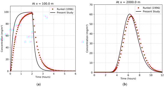
Figure 1. Results of concentration profiles of a non-reactive solute at (a) x = 100 m and (b) x = 2000 m for $v=0.1 \mathrm{m}/\mathrm{s}, D_L=5.0 {\mathrm{m}}^2/\mathrm{s}, t_c=2 \mathrm{h}, A=10 {\mathrm{m}}^2, C_0=100 (\mathrm{m}\mathrm{g}/{\mathrm{m}}^3)$. The plots illustrate MP concentration as a function of time t (hours). The solid black line represents the analytical solution derived in this study, while the red dotted line represents the numerical benchmark from Runkel [25]. The comparison is presented at two downstream distances: (a) x = 100 m and (b) x = 2000 m.

It is important to note that this validation serves as a baseline verification of the core advection-dispersion mechanics. The conventional model (Equation (21)) assumes non-reactive behavior (d = 0, λ = 0). To demonstrate the necessity of the modified equations for plastic wastes, which incorporate sinking and removal, a direct graphical comparison between the conventional and modified models (Figure 2). This comparison highlights the significant deviations in transport behavior when polymer-specific dynamics are considered.

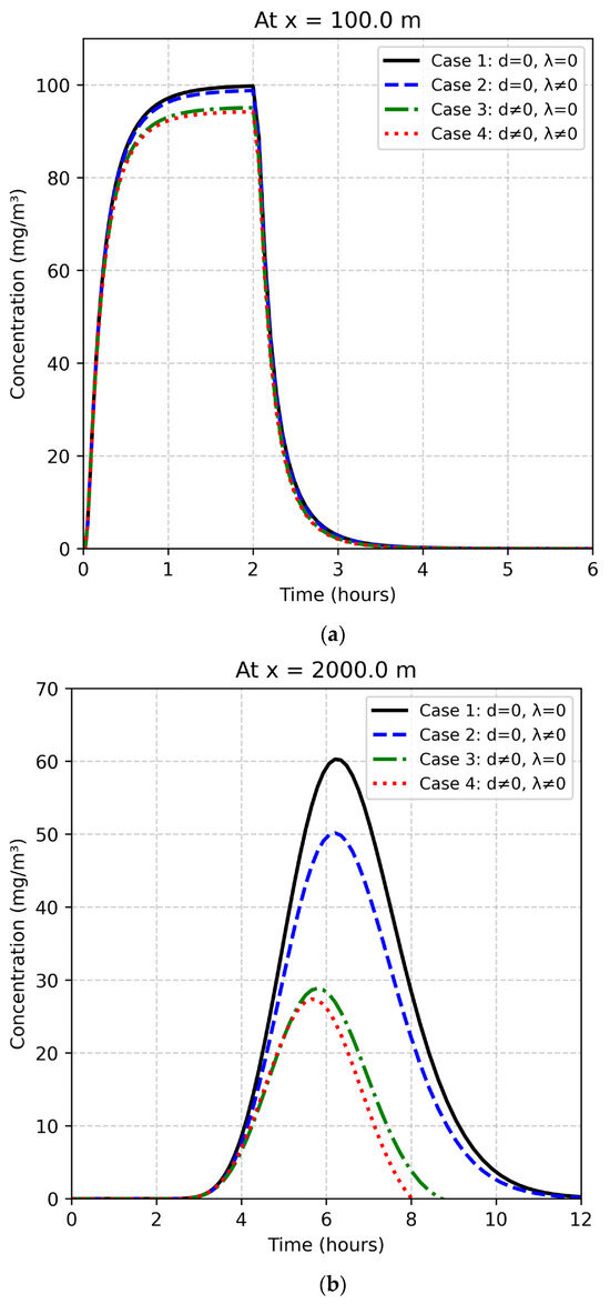
Figure 2. Graphical comparison of concentration profiles between the conventional model (Case 1, black line) and the modified plastic model (Cases 2–4), incorporating sinking (d) and removal (λ). (a) At x = 100 m: The conventional model shows the highest peak concentration, illustrating the overestimation risk when sinking/removal is ignored. (b) At x = 2000 m: The modified model demonstrates a significant “stretching” and reduction in the plume due to the cumulative effect of the modified terms over distance. Parameters:$v=0.1 \mathrm{m}/\mathrm{s}, D_L=5.0 {\mathrm{m}}^2/\mathrm{s}, C_0=100 \mathrm{m}\mathrm{g}/{\mathrm{m}}^3, t_c=2 \mathrm{h}, A=10 {\mathrm{m}}^2$ and $d=0.00005, \lambda =0.00001.$ Note: Values of d and λ are assumed for this study, and they are intended to capture the net effect of complex physical and biological processes.

3. Results and Discussion

3.1. Physical Behavior of the Modified Transport Model

The solution (30a,b) describes the concentration of MPs in a river system over time and space, accounting for advection (transport by flow) and dispersion (spreading due to turbulence), sinking to sediment, and removal processes. It tells a story of how plastic pollution spreads, moves, and eventually disappears from the river water.

Case 1: This part of the solution describes what happens while plastic is actively being dumped or washed into the river from a specific point. As we know, the plastic does not just stay in one spot. The river’s current pushes it downstream, creating a moving plume of pollution. The front edge of this plume travels at the same speed as the river’s flow. As this plume moves, it does not stay neat and tight. The turbulence and swirling motions in the river cause the plastic to spread both forward and backward, making the polluted plume longer and more diluted as it travels. While the plume is moving and spreading, it is also shrinking. This is because some plastic particles are heavy and slowly sink to the riverbed, like sand. Other particles are gradually broken down by sunlight, water, and tiny microbes, though this is often a very slow process for plastics. So, during an active spill, we have a moving, stretching, and shrinking plume of plastic pollution traveling down the river.

Case 2: This part of the solution describes what happens after the source of the pollution is turned off. Even after new plastic stops entering the river, the plume that was already in the water keeps moving downstream. With no new plastic being added, the entire plume continues to stretch and shrink. The plastic particles keep sinking to the bottom and breaking down. This means the overall amount of plastic in the water steadily decreases. The solution (Equation (31)) shows that plastic does not just vanish the moment the pollution stops. It can travel a very long way, continuing to affect the river environment for miles downstream. The “tail” of the polluted plume can be very long, meaning a river can show signs of contamination long after the original source has been dealt with.

3.2. Comparative Analysis of Transport Paradigms

Figure 2a,b provides a direct graphical comparison of MP transport behavior under two distinct paradigms: the conventional solute model versus the modified plastic-specific model. We consider four cases to isolate the effects of the modified terms:

Case 1. $d=0, \lambda =0.$(Indicates no sinking or removal of MPs).

Case 2. $d=0, \lambda \ne 0.$(Indicates removal but no sinking of MPs).

Case 3. $d\ne 0, \lambda =0.$ (Indicates sinking but no removal of MPs).

Case 4. $d\ne 0, \lambda \ne 0.$(Indicates both sinking and removal of MPs).

Figure 2a illustrates that while the conventional model (Case 1) maintains high peak concentrations, the modified models (Cases 3 and 4) show a clear reduction in peak height due to the sink terms. It is observed that a rapid increase in concentration starting at $t=0$ and concentrations peak around $t=2$ h (when the pollution pulse ends). After the peak, concentrations gradually decrease over time, and such variation in decrease is found almost the same for all the cases when $t>2$ h. However, the peak rate varies among cases, with Cases 1 and 2 showing the highest peak rate and Cases 3 and 4 showing the lowest peak rate between the time frame 0 and 2 h.

Also, Figure 2b shows the concentration profiles for all cases at x = 2000 m. It can be seen that concentration profiles show delayed behavior compared to Figure 2a, with concentrations starting to rise around $t=4 \mathrm{t}\mathrm{o} 5$ h. This delay indicates the travel time of the MPs from $x = 100 \mathrm{m} \mathrm{t}\mathrm{o} 2000 \mathrm{m}$. It is also seen that peak concentrations occur around $t=6$ h for all cases. However, all peaks are broader and lower than at $x=100 \mathrm{m}$, and this is due to the dispersion during transport of MPs. Also, Case 1 shows the highest level of concentration (~60 mg/m³) when we consider the sinking (d) and removal (λ) of MPs are absent. Next, Case 2 shows the second-highest level of concentration (~50 mg/m³) when we only consider the removal (λ) of MPs. Additionally, case 3 shows the third-highest level of concentration (~29 mg/m³) when we only consider the sinking (d) of MPs. Finally, case 4 shows the lowest pick of concentration (~28 mg/m³) when we introduced both sinking (d) and removal (λ) of MPs. Finally, all these findings suggest that, at the farthest points, the effects of sinking and removal are more pronounced due to the longer travel time. Also, sinking has a higher impact on concentration than removal.

3.3. Sensitivity of Transport Dynamics to Removal and Sinking

3.3.1. Impact of Removal Rates

Figure 3a shows the variation in concentration profiles with different removal rates (λ) for a fixed sinking rate (d = 0.00005) at x = 100 m. The result shows that all cases have nearly identical peak concentrations because removal has minimal time to act during the initial pulse. Also, all cases show nearly identical peak concentrations (~95$\mathrm{m}\mathrm{g}/{\mathrm{m}}^3$) that indicate that removal has minimal effect during the initial pulse phase, and then all cases show a gradual decline after the peak. Figure 3b shows a delayed arrival compared to x = 100 m, with concentrations starting to rise around t = 4–5 h and peak concentrations occurring around t = 6 h, which is later than at x = 100 m. Also, λ = 0.00005 shows the highest peak concentration (~35 $\mathrm{m}\mathrm{g}/{\mathrm{m}}^3$) and λ = 0.00001 shows the lowest peak concentration (~27 $\mathrm{m}\mathrm{g}/{\mathrm{m}}^3$). The lowest removal rates (λ = 0.00001) show the most dramatic reduction in concentration, indicating that removal has a cumulative effect over distance and time. It happens because a higher removal rate breaks down more MPs over time through chemical processes.

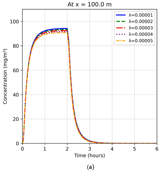
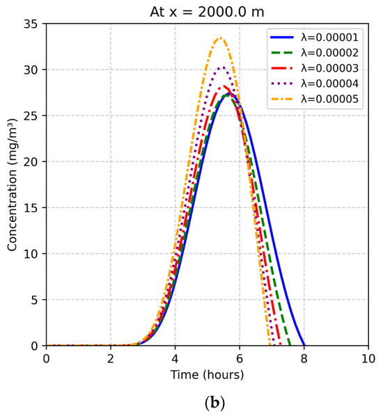
Figure 3. Variation in concentration profiles for different λ when d = 0.00005. (a) at x = 100 m; (b) at x = 2000 m.

3.3.2. Impact of Sinking Rates

Figure 4a shows MP transport through a river system under five different scenarios, comparing the effects of varying sinking rates (d) while keeping the removal rate (λ) fixed at x = 100 m. We observe that all the cases show a rapid increase in concentration starting at t = 0 and concentrations peak around t = 2 h (when the pollution pulse ends). After the peak, concentrations gradually decrease over time. Results reveal that d = 0.00001 shows the highest peak concentration and d = 0.00005 shows the lowest peak concentration. Overall, differences between cases are relatively small because the travel time is short, limiting the time available for sinking to remove MPs from the river. Figure 4b shows a delayed arrival compared to x = 100 m, with concentrations starting to rise around t = 4–5 h and peak concentrations occurring around t = 6 h, which is later than at x = 100 m. Also, d = 0.00001 shows the highest peak concentration (~32 $\mathrm{m}\mathrm{g}/{\mathrm{m}}^3$) and d = 0.00005 shows the lowest peak concentration (~27 $\mathrm{m}\mathrm{g}/{\mathrm{m}}^3$). The highest sinking rate (d = 0.00005) shows the most dramatic reduction in concentration, indicating that sinking has a cumulative effect over distance and time. It happens because a higher sinking rate removes more MPs from the water over time through settling on the riverbed. It suggests that sinking is an effective mechanism for reducing the long-term presence of MPs in the water. In addition, lower sinking rates allow MPs to remain suspended in the water for longer periods and travel greater distances.

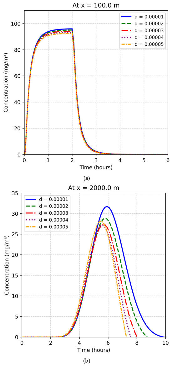
Figure 4. Variation in concentration profiles for different d when λ = 0.00003. (a) At x = 100 m; (b) At x = 2000 m.

3.4. Environmental Implications and Mechanism Dominance

A direct comparison of Cases 2 (removal only) and 3 (sinking only) in Figure 2 reveals a distinct grading in removal effectiveness. Although removal (λ) acts uniformly over time to reduce the total mass of MPs, it does not alter the physical residence time of the remaining particles in the water column as drastically as sinking (d). Our analysis indicates that sinking is the dominant mechanism for reducing aqueous concentration, particularly at higher rates (d > 0.00005). This suggests that for dense polymers (e.g., PVC, PET), the primary risk shifts from downstream transport (where plastics enter the ocean) to local sediment accumulation, where they pose long-term threats to benthic organisms. However, removal acts as a global mass reducer but is too slow to prevent significant downstream transport during the initial pulse phase.

A significant finding from the comparative analysis is the “stretching” of the concentration plume in the modified ADE compared to the conventional model. As shown in Figure 2b, the conventional model predicts a sharp, high-amplitude pulse. However, when sinking is introduced, the peak concentration is dampened, and the tail of the curve extends over a longer duration. This implies that conventional pollutant models significantly underestimate the exposure time of aquatic ecosystems to MPs.

Comparative Analysis

The modified ADE model is most suitable for “dilute” suspensions where the presence of MPs does not significantly alter the flow dynamics of the river. It is computationally efficient and ideal for risk assessment of standard pollution levels where transport is primarily driven by fluid velocity. The multi-phase model is essential for scenarios involving high-density plastic spills or wastewater effluent discharges with high particulate loads. In these scenarios, the momentum transfer from the particles to the fluid can potentially alter flow velocity and wave propagation. This model captures the complex, non-linear feedback that is neglected in standard advection-dispersion frameworks.

We have obtained a closed-form inverse Laplace transform for the coupled system (Equations (35) and (43)), which is analytically challenging, but the structure of the solution in the Laplace domain provides critical physical insight. In Equation (43), the influence of the particle concentration on the water level is driven by the integral term involving the coupling coefficient ω. This implies that as the density of the MP suspension increases, the effective momentum of the fluid is modified, which leads to a suppression of wave amplitudes compared to a clean water flow. This confirms that for ‘dense’ spills, the flow dynamics cannot be decoupled from the particle phase. The analytical solution provided here allows for the direct calculation of this feedback that serves as a theoretical tool to determine the maximum safe particle loading before hydraulic effects become significant.

3.5. Reconciliation with Field Observations and Broader Implications

The mathematical framework presented in this study offers a theoretical bridge between hydrodynamic transport and the empirical observations of MP distribution reported in recent field studies. Our findings, particularly regarding the dominance of the sinking mechanism, reconcile effectively with existing estimates of riverine MP transport. First, our modified ADE model highlights that sinking (d) is the primary driver for reducing aqueous concentrations (Figure 2, Figure 3 and Figure 4). This theoretical prediction aligns perfectly with the disparity often observed between surface water and sediment concentrations in field surveys. For example, studies have reported significantly higher MP abundances in sediments compared to surface water [11,12]. Our model attributes this discrepancy directly to the sink term (d) and suggests that as MPs move downstream, dense polymers settle out of the water column. This validates our model’s foundation that rivers act not just as transport pathways, but as critical accumulation zones for benthic ecosystems. Second, our results demonstrate the “long-tail” effect of MP plumes (Figure 2b), where concentrations persist long after the pollution pulse has ceased. This finding contextualizes the permeating presence of MPs in remote or downstream ecosystems. Also, researchers detected MPs in remote high-latitude lakes and in the guts of fish far from direct sources [6,10]. Our model supports the hypothesis that short-term urban discharge events can lead to prolonged downstream exposure due to the coupled advection–dispersion dynamics. Finally, the differentiation between removal (λ) and sinking (d) in our model provides a mechanistic explanation for polymer-specific distribution. Our analysis shows that removal has a negligible effect during the initial pulse phase but acts cumulatively over distance. This helps explain why durable polymers like Polyethylene (PE) and Polypropylene (PP) are frequently found in water samples [13,14], which remain dominant in the water column, whereas denser polymers like PVC and PET [17] are more likely to settle rapidly. Therefore, if we can adjust the sinking rate parameter, then our model can be used to predict the distinct transport fates of different polymer types.

Our results confirm that for persistent microplastics, the transport dynamics characterized by first-order sinking mirror the long-established behavior of suspended sediments and particle-bound reactive chemicals in rivers. As observed in chemical transport modeling, the ‘loss’ term d acts as a permanent sink, leading to the exponential decay of aqueous concentration and the accumulation of mass in the bed sediment.

4. Conclusions

Due to global population growth, the use of plastic has increased manifold, which has also led to an increase in the presence of MPs. Therefore, it is the right time to curb its use. The most important thing for this is to understand the flow pattern of MPs within the aquatic system and its effect on the surface water and the waterbed. We also need to identify effective control strategies to curb the use of MPs and to lessen the harmful effects of MPs on the environment. In these circumstances, a mathematical model can be very helpful, and hence we developed a mathematical model in terms of a modified advection diffusion equation by considering sinking, removal, and multi-phase dynamics to better understand the spread mechanism of MPs within the water body. Our study suggests that the effect of removal is negligible during the early pulse phase, but it has an increasingly cumulative impact over distance and time. Our results further depicted that a lower sinking rate has minimal impact, whereas a higher sinking rate has a far-reaching impact on the accumulation of MPs in riverbeds.

5. Limitation and Future Research Direction

• The current model treats MPs as a continuum with representative sinking and removal rates. However, in nature, MPs exhibit a wide variety of shapes (e.g., fibers, fragments, films), sizes, and polymer compositions. These physical characteristics significantly influence drag, buoyancy, and settling velocities in ways that a bulk parameterization cannot fully capture. Future models should aim to incorporate polydisperse size and shape distributions.
• The model focuses on abiotic transport and does not account for biological processes such as biofouling or the ingestion and active transport of MPs by living organisms. Furthermore, complex hydrological events, such as sediment redistribution during rising water levels, storm surges, and interactions in coastal zones, are not included in the current analytical framework.
• Future work should integrate these analytical findings into numerical frameworks that can handle the non-uniform geometry of natural channels. Additionally, the multi-phase model presented here requires further extension to fully capture complex flow-particle feedback in heterogeneous environments.
• The initial concentration $C_0$ was estimated using a regression based on socio-economic factors. Future studies should incorporate direct field measurements or remote sensing data to refine these source loading estimates.
• A significant limitation of the modified ADE approach is that it treats the sediment as a permanent sink. The model assumes that once MPs settle, they are permanently removed from the water phase. Consequently, this approach cannot answer open questions regarding bed sediment transport, remobilization, or resuspension under high turbulence or flood events. Future work should couple this analytical framework with a sediment transport model to capture the dynamic exchange between the water column and the riverbed.
• This study utilizes representative parameters to illustrate the analytical solution; the modified ADE is designed to accept site-specific input data. Future applications of this model should incorporate empirically determined sinking rates specific to the polymer types and hydraulic conditions of the study river.
• Our model treats the sinking rate as a first-order parameter; therefore, for fibers, d should be interpreted as an ‘effective’ settling velocity that must be carefully calibrated against monitoring data. Future studies are required to distinguish between the ‘suspension’ and ‘sedimentation’ regimes for fibers to improve the accuracy of bulk transport models.

References

- Strokal, M.; Vriend, P.; Bak, M.P.; Kroeze, C.; van Wijnen, J.; van Emmerik, T. River export of macro- and microplastics to seas by sources worldwide. Nat. Commun. 2023, 14, 4842. [Google Scholar] [CrossRef]
- Xia, F.; Yang, W.; Zhao, H.; Cai, Y.; Tan, Q. Occurrence characteristics and transport processes of riverine microplastics in different connectivity contexts. npj Clean Water 2025, 8, 1. [Google Scholar] [CrossRef]
- Barrantes, L.A.; Baar, A.; Fernandez, R.; Hackney, C.; Parsons, D.; Dorrell, R. Modelling the transport and deposition of sediment-microplastics fluxes in a braided river, using Delft3D. Philos. Trans. A 2025, 383, 20240442. [Google Scholar] [CrossRef]
- Bhowmik, A.; Saha, G. Microplastics in the Rural Environment: Sources, Transport, and Impacts. Pollutants 2026, 6, 3. [Google Scholar] [CrossRef]
- Bhowmik, A.; Saha, G. Microplastics in Our Waters: Insights from a Configurative Systematic Review of Water Bodies and Drinking Water Sources. Microplastics 2025, 4, 24. [Google Scholar] [CrossRef]
- Qin, Y.; Su, Y.; Zhang, Y.; Li, T.; Liu, J.; Wang, H.; Diao, X. Spatial heterogeneity of microplastics and ecological risk assessment based on detection of seawater and fish in typical coastal region in Hainan. Mar. Pollut. Bull. 2026, 223, 118942. [Google Scholar] [CrossRef]
- Jeylaputheen, M.A.; Sekar, S.; Perumal, M.; Parthiban, A.; Roy, P.D.; Elzain, H.E.; Kamaraj, J. Urbanization increases microplastic pollution in beach sediments along the Chennai Coast, South India. Mar. Pollut. Bull. 2026, 224, 119137. [Google Scholar] [CrossRef]
- Lu, H.; Mokarram, M. Global analysis of mineral aerosol and industrial effects on lake water quality using spectral indices and machine learning. Water Res. 2025, 290, 125055. [Google Scholar] [CrossRef] [PubMed]
- Li, Q.; Bai, Q.; Zheng, R.; Li, P.; Liu, R.; Yu, S.; Liu, J. Mass concentration, Spatial Distribution, and Risk assessment of Small Microplastics (1–100 μm) and Nanoplastics (<1 µm) in the Surface Water of Taihu Lake, China. Environ. Res. 2025, 285, 122214. [Google Scholar] [CrossRef]
- Ryan, A.C.; Maselli, V.; Kelly, N.E.; Walker, T.R. Atmospheric deposition drives microplastic contamination in remote lakes of Newfoundland, Canada. Sci. Total. Environ. 2025, 1003, 180762. [Google Scholar] [CrossRef]
- Manik, M.; Hossain, M.T.; Pastorino, P. Characterization and risk assessment of microplastics pollution in Mohamaya Lake, Bangladesh. J. Contam. Hydrol. 2025, 269, 104487. [Google Scholar] [CrossRef]
- Mutlu, T.; Ceylan, Y.; Baytaşoğlu, H.; Gedik, K. Characterization of microplastics in sediments and surface waters of Turkish lakes. J. Contam. Hydrol. 2025, 272, 104576. [Google Scholar] [CrossRef]
- Arcadio, C.G.L.A.; Albarico, F.P.J.B.; Hsieh, S.L.; Chen, Y.T.; Bacosa, H.P. Microplastic distribution in the surface water and potential fish uptake in an oligotrophic lake (Lake Mainit, Philippines). J. Contam. Hydrol. 2025, 273, 104603. [Google Scholar] [CrossRef]
- Li, K.; Zhao, R.; Meng, X. Spatio-temporal distribution of microplastics in surface water of typical urban rivers in North China, risk assessment and influencing factors. J. Contam. Hydrol. 2025, 273, 104626. [Google Scholar] [CrossRef]
- Fu, Y.; Deng, H.; Gong, W.; He, J.; Zhang, L.; Ni, Y. Tidal intensity and suspended sediment concentration drive microplastic distribution in the Pearl River Estuary: Insights from remote sensing retrieval. Environ. Pollut. 2025, 390, 127497. [Google Scholar] [CrossRef]
- Wu, Y.; Chen, J.; Zhang, L.; Wu, C.; Zhou, C.; Chen, Y.; Hou, Z.; Wang, Q. Microplastic Distribution in an Urban-Influenced Plateau Lake: A Case Study of Qionghai Lake, China. J. Environ. Chem. Eng. 2025, 14, 120749. [Google Scholar] [CrossRef]
- Suresh, N.; Joseph, M.M. Microplastic Pollution and its Ecotoxicological Impact: Evidence from Vembanad Lake and Zebrafish Studies. Reg. Stud. Mar. Sci. 2026, 93, 104705. [Google Scholar] [CrossRef]
- Ervik, H.; Mészey, A.; Røsvik, A.; Jenssen, B.M. Organic contaminants and toxic elements in marine plastic debris, water and sediments in small freshwater lakes in a Norwegian coastal archipelago. Heliyon 2026, 12, e44232. [Google Scholar] [CrossRef]
- Kumar, A.; Poddar, V.K.; Sardar, S.; Mistri, A.; Srivastava, A. Microplastic pollution in rivers and lakes of India: Sources, ecotoxicological impacts, and removal strategies. NanoImpact 2025, 41, 100604. [Google Scholar] [CrossRef]
- Hassan, M.A.; Mahmud, D.S.; Shammi, M.; Tareq, S.M. Does Tourism Enhance Microplastic Pollution in the Ecologically Critical Areas of Bangladesh? Evidence from Tanguar Haor, Kaptai Lake, and the Sundarbans. J. Hazard. Mater. Adv. 2025, 21, 100929. [Google Scholar] [CrossRef]
- Pulikkoden, A.K.; Qashqari, M.; Kannaiyan, N.; AlAqad, K.M.; Meleppura, R.; Gopalan, J.V.; Premlal, P.; Manikandan, K.P.; Maneja, R.H.; Nazal, M.K.; et al. Microplastics in Saudi Arabia: Environmental occurrence, research gaps, and challenges in extreme conditions. J. Hazard. Mater. Plast. 2025, 2, 100018. [Google Scholar] [CrossRef]
- Arbeloa, P.D.N.; Marzadri, A. (Modeling the transport of microplastics along river networks. Sci. Total Environ. 2024, 911, 168227. [Google Scholar] [CrossRef] [PubMed]
- Arfken, G.B.; Weber, H.J.; Harris, F.E. Mathematical Methods for Physicists: A Comprehensive Guide, 7th ed.; Academic Press: San Diego, CA, USA, 2011. [Google Scholar]
- Duffy, D.G. Green’s Functions with Applications, 2nd ed.; Chapman and Hall/CRC: Boca Raton, FL, USA, 2015. [Google Scholar] [CrossRef]
- Runkel, R.L. Solution of the Advection-Dispersion Equation: Continuous Load of Finite Duration. J. Environ. Eng. 1996, 122, 830–832. [Google Scholar] [CrossRef]
Disclaimer/Publisher’s Note: The statements, opinions and data contained in all publications are solely those of the individual author(s) and contributor(s) and not of MDPI and/or the editor(s). MDPI and/or the editor(s) disclaim responsibility for any injury to people or property resulting from any ideas, methods, instructions or products referred to in the content. |
© 2026 by the authors. Licensee MDPI, Basel, Switzerland. This article is an open access article distributed under the terms and conditions of the Creative Commons Attribution (CC BY) license.