Solubility-Driven Prediction of Electrospun Nanofibers’ Diameters via Generalized Linear Models ^†

Abstract

Electrospinning is a versatile technique for producing polymer nanofibers whose morphology strongly influences their properties. This work developed predictive and inferential models for fiber diameter based on solution and process parameters. Polymer–solvent compatibility was described through cohesive energy-based solubility parameters such as Hansen and Flory–Huggins ($\chi$). Twenty Generalized Linear Models (GLMs) were trained using both the raw response (Y) and its natural logarithm (ln Y) under Gaussian, Gamma, and Inverse Gaussian distributions with different link functions. Models using ln Y showed better goodness-of-fit, with the Gamma distribution and identity link performing best. The final model, optimized via AIC-forward selection, achieved RMSE = 0.5862, Corr² = 0.7803, and MAPE = 0.0775. The Flory–Huggins parameter and solution concentration were identified as the most influential predictors, providing a reliable framework for controlling nanofiber diameter in electrospinning processes.

1. Introduction

Electrospinning is an electrostatic nanofiber fabrication technique. Fibers can be made from many substrates, such as molten salts, composite materials, and mainly polymer solutions. Polymer solutions are made of polymers dissolved in a proper solvent. Many of the parameters of polymer solutions, such as viscosity and superficial tension, impact the morphology of the fiber [1], and these are strongly related to polymer-solvent system affinity [2].

The molecular compatibility of the polymer solution system can be determined via solubility parameters, e.g., Hansen (${\delta }_d,{\delta }_p,{\delta }_h$), Hildebrand ($\delta$), and Flory–Huggins ($\chi$), which describe the cohesion energy likeliness as well as the molecular ordering and interaction strength between polymer and solvent through the Relative Energy Difference (RED) of the species [3]. Figure 1 shows, in yellow and blue, the operational and solution parameters, respectively, for the electrospinning process that affects the nanofiber diameter.

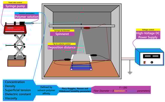
Figure 1. Experimental setup and parameters governing the fiber diameter in the electrospinning process.

Hildebrand first introduced the concept of solubility parameters in 1950 to describe miscibility between species based on their cohesive energy. He proposed that substances with similar solubility parameter values ($\delta$) are likely to mix without phase separation [4]. Later, Hansen, from 1995 to 2000, refined this concept by identifying that solubility depends on different types of molecular interactions. He divided the total cohesive energy into three components—dispersive (${\delta }_d$), polar (${\delta }_p$), and hydrogen bonding (${\delta }_h$)—and represented them in a three-dimensional coordinate system to assess compatibility between species [3]. The relationship between the Hansen and Hildebrand parameters is given by

$$\delta =\sqrt{{\delta }_d^2+{\delta }_p^2+{\delta }_h^2}$$

(1)

The three-dimensional distance (Ra) and the RED can quantify the affinity of a solvent–polymer system:

$$Ra=\sqrt{4{{(\delta }_{d2}-{\delta }_{d1})}^2+{{(\delta }_{p2}-{\delta }_{p1})}^2+{{(\delta }_{h2}-{\delta }_{h1})}^2}$$

(2)

Then

$$\mathrm{R}\mathrm{E}\mathrm{D}={\displaystyle \frac{Ra}{R_0}}$$

(3)

where

• Ra = three-dimensional distance between solvent–polymer coordinates (MPa^1/2).
• ${\delta }_{d1}, {\delta }_{p1}, {\delta }_{h1}$ = Hansen solubility parameters of the polymer (MPa^1/2).
• ${\delta }_{d2}, {\delta }_{p2}, {\delta }_{h2}$ = Hansen solubility parameters of the solvent (MPa^1/2).
• R₀ = radius of interaction of the polymer (MPa^1/2).
• RED = Relative Energy Difference between the species. Systems with RED ≤ 1 are considered miscible, while RED > 1 are not.

Shrutidhara Sarma employed voltage, collector distance, and feed rate, together with the Hansen solubility parameters of the polymer solution, to evaluate polymer–solvent affinity through the Relative Energy Difference (RED) and predict the diameter of polyvinylidene fluoride (PVDF) fibers using artificial intelligence. The models were of the black-box type, meaning the relationship between inputs and outputs was not explicitly defined [5]. Model performance was assessed through the determination coefficient (R²), representing the percentage of explained variance, and the Root Mean Squared Error (RMSE), which measures the average prediction error [6]. The best model, a Gradient Boosting Regressor (GBR), achieved an R² of 0.98 and an RMSE of 76.37 nm. SHapley Additive exPlanations (SHAP) analysis revealed that feed rate was the most influential process variable, followed by polymer concentration and the Flory–Huggins interaction parameter [7].

Figure 2 shows the lignin sphere of Hansen compared to proper (blue dots) and improper (red dots) solvents. The units for three axes are MPa^1/2.

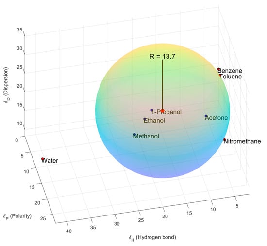
Figure 2. Three-dimensional sphere for lignin and various solvents.

Mohammad Golbabaei designed classification (qualitative) and prediction (quantitative) black-box models to determine the fiber diameter and electrical conductivity. For the quantitative diameter prediction, the best performing model was an Artificial Neural Network (ANN), which reached an amazingly high R² value of 0.8. The dataset used consisted of chitosan, polyvinyl alcohol (PVA), polycaprolactone (PCL), and gelatin, among other elements [8].

While there has been work that has successfully designed models to determine nanofiber diameter, there is yet to be a white-box model that explains a direct relationship, f(X₁,X₂,…) = Y, between solution and operation parameters and the nanofiber diameter of electrospun fibers.

Ordinary Least Squares (OLS) classic linear regression models assume that data follow a Gaussian distribution when trained, where the mean, median, and mode coincide and observations are symmetrically distributed (hence the non-dependence of mean on variance) [9]. However, many phenomena—such as electrospinning—are not likely to exhibit this behavior due to their high degrees of freedom. Generalized Linear Models (GLMs) are powerful tools for analyzing non-Gaussian data, as they extend classical regression by incorporating distributions from the exponential family, expressed as

$$\mathrm{E}\left[Y\right]=g(\mu )=\eta =X\beta$$

(4)

where

• E[Y] = expected value of Y;
• g($\mu$) = link function;
• $\eta$ = X$\beta$ = linear predictor.

The link functions transform the linear predictor matrix–input to fit the response variable–output, where $\beta$ is calculated via Maximum Likelihood Estimation (MLE). This approach identifies the coefficients that maximize the likelihood of observing the given data based on the assumed probability density function. As a result, the estimated coefficients describe the relationship between predictors and the response within the chosen link–distribution framework [10]. Table 1 summarizes the link functions associated with each exponential-family distribution. The canonical link, indicated in the table footnotes, represents the function that best fits each distribution; however, alternative link–distribution combinations commonly used in practice are also included [10].

Table 1. Link function relations for exponential probability distribution family.

Link Function	$\mathit{g}(\mathit{\mu }$$)=\mathit{\eta }$$=\mathit{X}\mathit{\beta }$	${\mathit{g}}^{-1}(\mathit{\eta }$$)=\mathit{\mu }$	Response Variable Y	Commonly Used Distributions
Identity	$\mu$	$\eta$	Continuous	Gaussian 1, Poisson, Gamma, Inverse Gaussian
Log	$\ln \mu$	$e^{\eta }$	Continuous	Gaussian, Poisson 2, Gamma, Inverse Gaussian
Inverse	${\mu }^{-1}$	${\eta }^{-1}$	Continuous	Gaussian, Poisson, Gamma 3, Inverse Gaussian
Inverse squared	${\mu }^{-2}$	${\eta }^{-2}$	Continuous	Inverse Gaussian 4
Square root	${\mu }^{-{\displaystyle \frac{1}{2}}}$	${\eta }^{-{\displaystyle \frac{1}{2}}}$	Discrete	Poisson
Logit	$\ln \left({\displaystyle \frac{\mu }{1-\mu }}\right)$	${\displaystyle \frac{e^{\eta }}{1+e^{\eta }}}$	Discrete	Bernoulli 5, Binomial 6
Probit	${\varphi }^{-1}\left(\mu \right)$	$\varphi \left(\eta \right)$	Discrete	Bernoulli, Binomial
Log-Log	$-\ln \left(-\ln \mu \right)$	$\mathrm{e}\mathrm{x}\mathrm{p}(-\exp \left(-\eta \right))$	Discrete	Bernoulli, Binomial
C-Log-Log	$\ln \left(-\ln (1-\mu )\right)$	$1-\mathrm{e}\mathrm{x}\mathrm{p}(-\exp \left(\eta \right))$	Discrete	Bernoulli, Binomial

¹ Identity is the canonical link for Gaussian distribution. Default framework used in OLS. ² Log is the canonical link for Poisson distribution. ³ Inverse is the canonical link for Gamma distribution. ⁴ Inverse squared is the canonical link for Inverse Gaussian distribution. ^5,6 Logit is the canonical link for Bernoulli and Binomial distributions.

2. Materials and Methodology

2.1. Data Collection

A meta-analysis of electrospun nanofibers was conducted, searching for common synthetic and non-synthetic polymers used in electrospinning. The polymer Hansen parameters of solvent and polymer were used to calculate the RED of the system and the Flory–Huggins parameter, following Shrutidhara’s process [7]:

$$\chi ={\displaystyle \frac{M_{v}R{a}^2}{16.736RT}}$$

(5)

where

• $\chi$ = Flory–Huggins parameter;
• $M_v$ = molar volume (cm³/mol);
• Ra = three-dimensional distance between solvent–polymer coordinates (MPa^1/2);
• $R$ = 1.987 cal/mol K;
• T = temperature (K).

Figure 3 shows the total records of the polymers, while Table 2 shows the range of every X in the database.

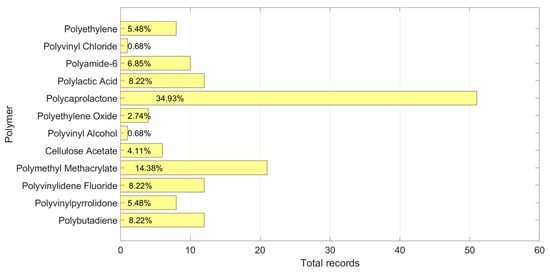
Figure 3. Number of records and percentages by polymer in the training database.

Table 2. Value ranges across Y’s and X’s in database.

Variable	Parameter	Values Range
Response variable (Y)	Fiber Diameter (nm)	45.0000–7670.0000
X1	RED	0.2416–1.2962
X2	Flory–Huggins Interaction Parameter (F_H)	0.0074–0.7752
X3	Jet speed-Velocity (cm/h)	6.0172–9417.4520 1
X4	Temperature (K)	293.1000–393.1000
X5	Syringe diameter (cm)	0.0260–0.4600
X6	Feed Rate (cm3/h)	0.1000–12.000
X7	Distance (cm)	6.0000–20.0000
X8	Voltage (kV)	5.5000–45.0000
X9	Polymer Concentration (wt%)	0.1000–22.0000
X10	Type of electrospinning	0, 1, 2 2

¹ Jet speed was calculated by continuity fluid law using Syringe Diameter (X₅) and Feed Rate (X₆). ² Categorical X: 1 and 2 are inner and outer polymers in coaxial electrospinning, respectively, while 0 means non-coaxial electrospinning.

2.2. Materials, Resources, and Process

Modeling was conducted in RStudio software v.2025.05.1+513 (Allaire, NJ, USA) [11]. Table 3 displays the main libraries used for data analysis and modeling.

Table 3. Libraries’ functions used throughout data processing.

Library	Function/Syntaxis	Usage
stats	glm(formula, data, family(“link function”)) 1	Model training
car	residualPlots(model)	Check linearity across X’s
glmtoolbox	BoxTidwell(model, transf~variable)	Fix linearity across X’s 2
DHARMa 3	plot(simulateResiduals(model, seed))	Check normality of GLM
MASS	stepAIC(model, direction = c(“both”), k) 4	AIC/BIC variable reduction 5

¹ Default value for “formula” is “Y ~ .” which represents Y’s dependence on all X’s found in Table 1, while “family” can be either “gaussian”, “Gamma”, or “inverse.gaussian” for this work. ² Function output is better $\lambda$ value to which $X^{\lambda }$ more effectively fixes residual linearity in the model. ³ Diagnostics for Hierarchical Regression Models. ⁴ k-Parameter is a natural logarithm of database sample size ($\mathrm{l}\mathrm{n} n$) to simulate BIC variable selection. ⁵ Akaike Information Criteria (AIC) and Bayesian Information Criteria (BIC).

The electrospinning parameters and synthesis materials for experimental verification are presented in Table 4 and Table 5, respectively. Some variables are not shown since they were fixed to constant values to analyze the voltage variation on fiber diameter, such as syringe diameter—0.072 cm; velocity—491.219 cm/h; and temperature—297.150 K.

Table 4. Electrospinning parameters of PVA nanofibers.

Sample 1	PVA Concentration (wt%)	HAc 2 Concentration (wt%)	Feed Rate (mL/h)	Voltage (kV)	Distance (cm)
A	10.00	5.00	2.00	30.00	18.00
B	10.00	5.00	2.00	25.00	18.00
C	10.00	5.00	2.00	20.00	18.00

¹ All experimental samples were non-coaxial electrospinning (Type = 0). ² Acetic acid (HAc).

Table 5. Materials used for PVA polymeric solution synthesis.

Material	Description	Chemical Formula
Deionized water	Barnstead MicroPure ST Thermo Scientific-processed (Waltham, Massachusetts, USA)
Acetic Acid (HAc)	Reagent Grade (R.G.), Merck (Darmstadt, Germany)
Polyvinyl Alcohol	R.G., Merck (Darmstadt, Germany) Molecular Weight (M.W.) 89,000–98,000 99+% hydrolyzed

2.3. Inference Modeling

Twenty GLMs were trained using Gaussian, Gamma, and Inverse Gaussian families to evaluate the goodness-of-fit across different continuous response frameworks. The response variable was modeled as the natural logarithm of the fiber diameter (ln Y) to improve normality and variance stability; this assumption was later verified through the Box–Cox transformation test.

Cook’s distance, leverage, and box plots were used to identify influential records in the Y and X variables. Model assumptions were assessed through QQ-plots (Quantile-Quantile-plots), residual histograms, and DHARMa residual analyses to verify normality and homoscedasticity.

Box–Tidwell transformation tests were performed for each parameter to examine predictor linearity and determine whether the linearity in the model could be fixed or not by transforming X.

Variable selection was guided by the Akaike (AIC) and Bayesian (BIC) Information Criteria using forward, backward, and bidirectional procedures, with assumptions verified at each step.

2.4. Prediction Modeling

The best inference framework was applied to train models, including main, quadratic, and interaction effects. Data were split following an 80:20 ratio using the repeated hold-out sampling method, and AIC/BIC-based reduction was performed to obtain the most parsimonious and best-fitting models.

Model performance was evaluated through the Mean Squared Error (MSE) and its root (RMSE), Mean Absolute Error (MAE), and its Percentage (MAPE). The squared correlation coefficient (Corr²) between predicted and observed responses was also calculated to assess predictive accuracy.

2.5. Experimental Testing

The samples were prepared by dissolving 1 g of PVA in 8.5 g of deionized water previously acidified with 0.5 g of HAc and heated at 60 °C for 5 min. This mixture was then mechanically stirred for 15 h until complete dissolution. Electrospinning was conducted on the same day to ensure solution stability.

The morphology of the electrospun PVA fibers was examined using Scanning Electron Microscopy (SEM) (JSM-7800F, JEOL, Tokyo, Japan). Prior to imaging, the samples were coated with a thin gold layer (~10 nm) by sputtering at 20 mA for approximately 60 s. Micrographs were obtained at an accelerating voltage of 10 kV, with magnifications between 1000× and 100,000×.

3. Results and Discussion

3.1. Inference Modeling

Figure 4a shows the best transformation for the Box–Cox test, which determined that the best transformation for Y was $\lambda$ = −0.222 (p-value = 2.2 × 16⁻¹⁶). Logarithmic transformation ln(Y) was performed, giving $\lambda$ closeness to 0 and to simplify interpretation, as suggested by Remi Sakia [12].

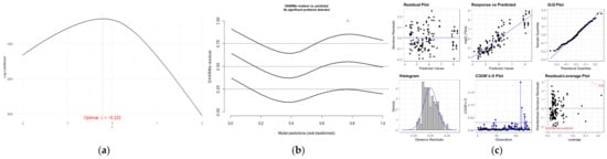
Figure 4. (a) Log-likelihood maximization for λ-transformation values, (b) DHARMa residuals, and (c) residual panel for Gamma($\mu$) model: response ln(Y).

The best goodness-of-fit framework was identified as the Gamma distribution with an identity link using the ln(Y)-transformed response. Figure 4b presents the DHARMa and Figure 4c shows the leverage and Cook’s distance plots, indicating no influential observations, except for record 113. This observation corresponds to the highest jet speed (X₃) in the dataset (noted as a red asterisk in the DHARMa plot); however, it remains within acceptable limits for both Cook’s distance and leverage.

3.2. Prediction Modeling and Experimental Verification

The best performing model, obtained by AIC forward reduction in Gamma($\mu$), and the transformed response ln(Y) of main effects + interactions was used to predict nanofiber diameter on Samples A, B, and C, shown in Table 4. Figure 5 displays SEM nanofibers as well as the distribution of their measured dimensions compared to their predicted dimensions. In orange the mean plus minus the deviation is presented ($\mu \pm \sigma$), while red dotted lines display lower (LB) and upper (UB) bounds of it.

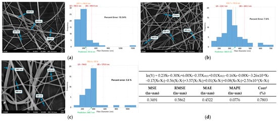
Figure 5. Real diameter represented by SEM analysis and fiber measured histogram vs. predicted for (a) sample A, (b) sample B, (c) sample C, and in (d) the simplified formula, as well as the metrics of the prediction model.

4. Conclusions

The developed GLM-based Gamma($\mu$) successfully predicted electrospun log-nanofiber diameters from solubility and process parameters, achieving strong correlation and low error. These results demonstrate the potential of interpretable statistical models to guide polymer–solvent selection and process optimization in electrospinning.

References

- Bhardwaj, N.; Kundu, S.C. Electrospinning: A fascinating fiber fabrication technique. Biotechnol. Adv. 2010, 28, 325–347. [Google Scholar] [CrossRef] [PubMed]
- Francis, L.F. Materials Processing: A Unified Approach to Processing of Metals, Ceramics and Polymers, 1st ed.; Elsevier: Amsterdam, The Netherlands, 2016; Volume 6. [Google Scholar]
- Hansen, C.M. Hansen Solubility Parameters: A User’s Handbook, 1st ed.; CRC Press LLC: New York, NY, USA, 2000. [Google Scholar]
- Hildebrand, J.H.; Scott, R.L. The Solubility of Nonelectrolytes, 3rd ed.; Science: New York, NY, USA, 1950; p. 488. [Google Scholar]
- Loyola-González, O. Black-box vs. white-box: Understanding their advantages and weaknesses from a practical point of view. IEEE Access 2019, 7, 154096–154113. [Google Scholar] [CrossRef]
- Starbuck, C. Linear Regression. In The Fundamentals of People Analytics; Springer: Berlin/Heidelberg, Germany, 2023; pp. 181–206. [Google Scholar]
- Sarma, S.; Verma, A.K.; Phadkule, S.S.; Saharia, M. Towards an interpretable machine learning model for electrospun polyvinylidene fluoride (PVDF) fiber properties. Comput. Mater. Sci. 2022, 213, 111661. [Google Scholar] [CrossRef]
- Golbabaei, M.H.; Varnoosfaderani, M.S.; Hemmati, F.; Barati, M.R.; Pishbin, F.; Ebrahimi, S.A.S. Machine learning-guided morphological property prediction of 2D electrospun scaffolds: The effect of polymer chemical composition and processing parameters. RSC Adv. 2024, 14, 15178–15199. [Google Scholar] [CrossRef] [PubMed]
- Socuéllamos, J.M. Modelos Lineales Generalizados, 1st ed.; Universidad Miguel Hernández: Elche, Spain, 2001; p. 247. [Google Scholar]
- Nelder, J.; Wedderburn, W. Generalized Linear Models. J. R. Stat. Soc. 1972, 135, 370–384. [Google Scholar] [CrossRef]
- Allaire, J.J. R: A Language and Environment for Statistical Computing; R Foundation for Statistical Computing: Vienna, Austria, 2025. [Google Scholar]
- Sakia, R. The Box-Cox Transformation Technique: A Review. J. R. Stat. Soc. 1992, 41, 169–178. [Google Scholar] [CrossRef]
Disclaimer/Publisher’s Note: The statements, opinions and data contained in all publications are solely those of the individual author(s) and contributor(s) and not of MDPI and/or the editor(s). MDPI and/or the editor(s) disclaim responsibility for any injury to people or property resulting from any ideas, methods, instructions or products referred to in the content. |
© 2025 by the authors. Licensee MDPI, Basel, Switzerland. This article is an open access article distributed under the terms and conditions of the Creative Commons Attribution (CC BY) license (https://creativecommons.org/licenses/by/4.0/).