Predicting the Window Opening State in an Office to Improve Indoor Air Quality ^†

Abstract

Window operation is among one of the most influential factors on indoor air quality (IAQ). In this paper, we focus on the modeling of the windows’ opening state in a real open-plan office with five windows. The IAQ of this open-plan office was monitored over a whole year along with the opening state of the windows. A k-Nearest Neighbor (k-NN) classification model was implemented, based on a long time series of both indoor and outdoor monitored environmental factors such as temperature and relative humidity, and CO₂ indoor concentration. In addition, the month, the day of the week and the time of the day were included. The obtained model for the window state prediction performs well with an accuracy of 92% for the training set and 86% for the testing set.

1. Introduction

Indoor air quality (IAQ) is, nowadays, an essential research topic, as we spend more than 90% of our time indoors [1]. The opening state of windows has an important influence on IAQ; therefore, it is necessary to understand and model the relationship between them [2].

Previous studies mostly used logistic regression to compute the correlation between the probability of a window opening and environmental stimuli to predict the probability of a window opening/closing event [3,4]. For this approach, all the observations need to be independent, and the outcomes of the model are usually complex equations which may not be easily understandable and interpreted.

In the last decades, many studies have used Machine Learning (ML) and their research application to the environment is not an exception. In 2014, D’Oca et al. tried to apply ML by using a data-mining approach to discover patterns of window opening and closing behavior in offices [5]. In this study, a huge amount of detailed data was needed and the authors mainly focused on obtaining distinct behavioral patterns of the window tilting angle, instead of for its opening state for a group of windows as was the case in our study. Many ML algorithms, such as Decision Trees, Support Vector Machines, k-Nearest Neighbor and Ensemble classification, can be applied for our study case. The k-NN classification is recommended as ‘a theoretically optimal method of classification’ [6]. Indeed, the best results were obtained on our case by using k-NN classification. To the best of our knowledge, this method has not yet been applied to predicting the state of window opening, but it has recently been used in a related topic of IAQ, which is occupancy detection [7]. This paper presents the ability of a k-NN classifier to predict the state of window opening in an open-plan office, as presented hereafter.

2. Methodology

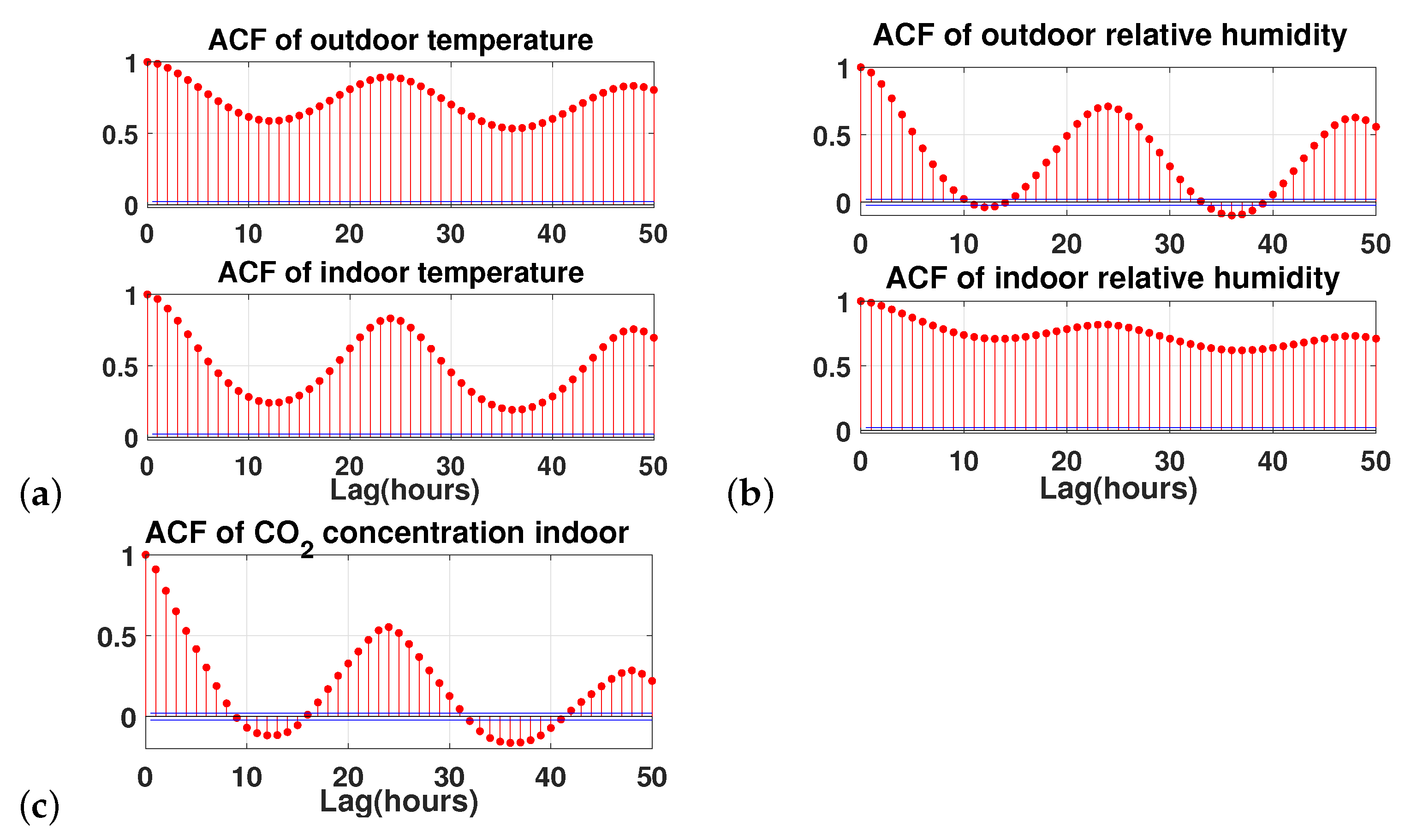
2.1. Study Case and Parameters Selection

The studied open-plan office is located in the suburban town of Champs-sur-Marne, France. The surface and the volume of the office are 132 m² and 364 m³, respectively; it is used by 6 to 15 people, from 8:00 a.m. to 6:00 p.m. from Monday to Friday.

Measurement devices were installed inside and outside the office. The monitoring was performed over a full year, in 2014. Temperature (T), relative humidity (RH), carbon dioxide (CO₂) and particulate matter were monitored every minute, during the whole year. The five windows of the office were equipped with sensors that detected each opening or closing event [8].

According to some previous studies, the outdoor temperature and indoor CO₂ concentration were the two most important variables in determining the probability of opening/closing windows, followed by indoor air temperature, and outdoor and indoor relative humidity [3,4,9]. In addition, non-environmental factors, that is, seasonal change, time of the day and personal preference, also affect the window-opening probability [10]. Thus, in our model, the following variables were used: month, day of the week, time of the day, indoor CO₂ concentration, and both indoor and outdoor temperature (T) and relative humidity (RH). The main statistics of these environmental parameters are displayed in Table 1.

Table 1. The statistics for the environmental parameters.

Features	Indoor CO2 (ppm)	Indoor T (${}^{\circ }$C)	Outdoor T (${}^{\circ }$C)	Indoor RH (%)	Outdoor RH (%)
Max value	1144	31.3	35.6	74.6	100.0
Min value	416.8	15	−4.3	18.3	26.9
Mean value	501.1	23	13.5	44.2	82.2
Median value	480.5	22.4	13.5	42.9	86.7
Std value	64.3	2.3	6	9.3	16.2

In order to obtain more information about the monitored time series, the autocorrelation function (ACF) was calculated (using hourly averaged data). The ACF of a time series $Y\left(t\right)$ provides a measure of the correlation between $y_t$ and $y_{t+k}$, where $k=0,\cdots ,K$ ($k\in \mathbb{Z}$, K is not larger than $T/4$) and $y_t$ is assumed to be the realization of a stochastic process. According to [11], the autocorrelation $r_k$ for lag k is:

$$r_k=\frac{c_k}{c_0},$$

(1)

where:

$$c_k=\frac{1}{T}\sum _{t=1}^{T-k}(y_t-\overline{y})(y_{t+k}-\overline{y})$$

(2)

and $c_0$ is the sample variance, $\overline{y}$ is the sample mean of the time series; T is the number of observations.

Figure 1 presents the ACFs for all the quantitative variables used in this study.

Figure 1. Autocorrelation values of environmental variables: (a) temperature, (b) relative humidity, and (c) Carbon dioxide concentration.

From the results presented in Figure 1, one can notice that the state of the environment at one sample (hour) has the highest correlation with the next sample. In other words, the previous hour of environmental data also has an important impact on the current information. Therefore, this implies that the previous hour of environmental data also has an important impact on the current state of the window. Hence, we decided to use the information on both the previous and current samples for the input to the predicting model.

We notice that the autocorrelation becomes zero after around 8 h for indoor CO₂ and outdoor RH. By contrast, indoor RH decreases very slowly. The same pattern can be found for outdoor, and also indoor, air temperature. This reveals the persistence of T and RH indoors, which means that a value at time t of the temperature or indoor relative humidity can have an impact on a value a long time later. We also note that the ACF of the CO₂ concentrations and RH outdoors becomes negative and remains at low levels, then switches back to positive values after a lag of 17 h. As for T outdoors and RH indoors, the autocorrelations persist in the positive for long delays. In general, temperatures and humidity depict the same structures of spectral variability as CO₂: two fundamental frequency peaks at (24 h)^–1 and (12 h)^–1. The ACF of CO₂ and outdoor RH alternates sign every 8 h on a lag of 24 h. This implies that, instead of using the information from the ’previous hour’, in the real-time system, we could use the values of the environmental data from ‘the previous 24 h’ as an input for this model, which are much easier to access than the ‘previous hour’ data for a real-time application.

2.2. Classification Model Implementation

The hourly averaged values of the selected parameters were used. A linear interpolation was applied in order to replace missing values. Then, the responses were categorized into four different groups, labelled as follows:

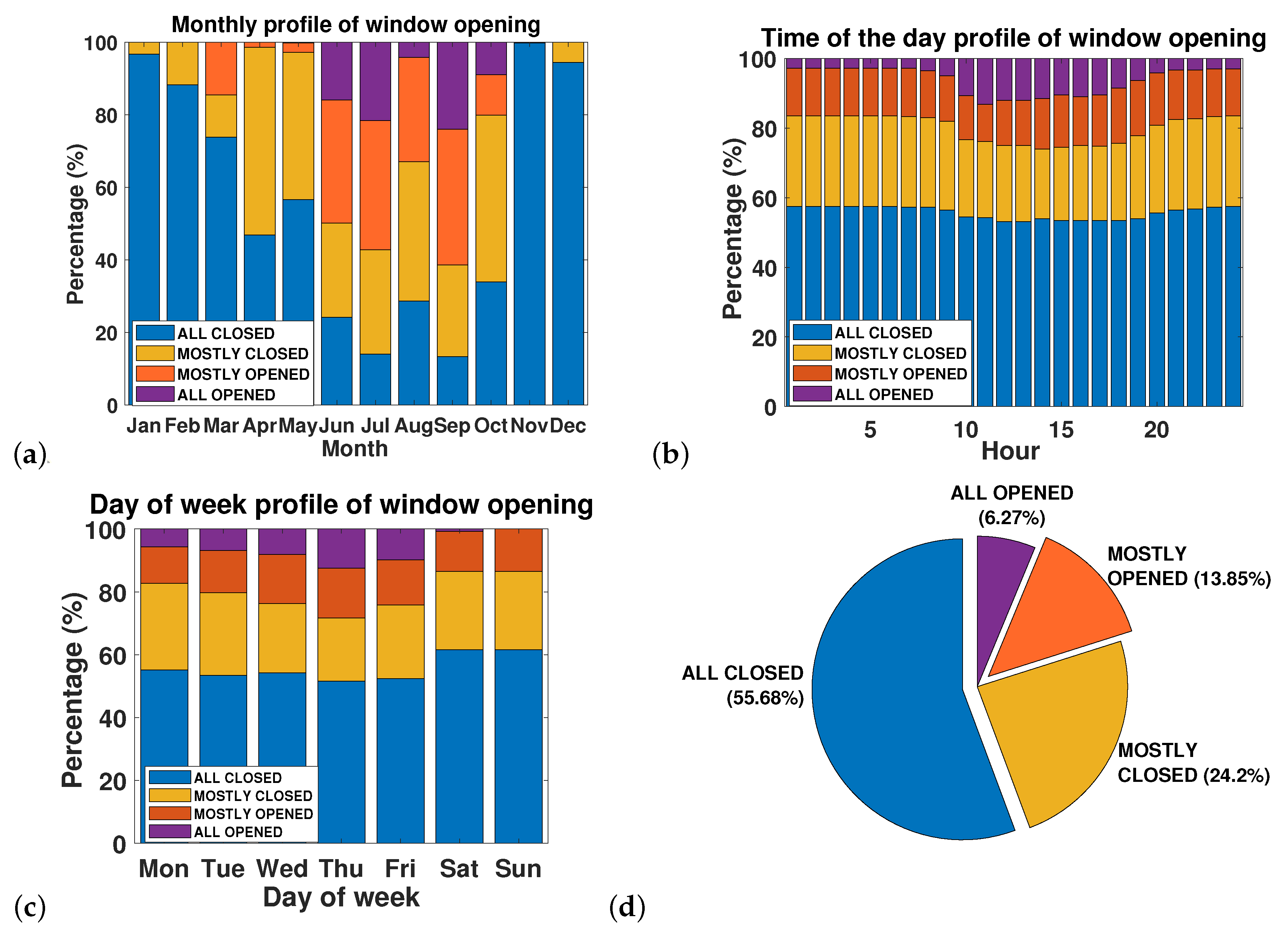
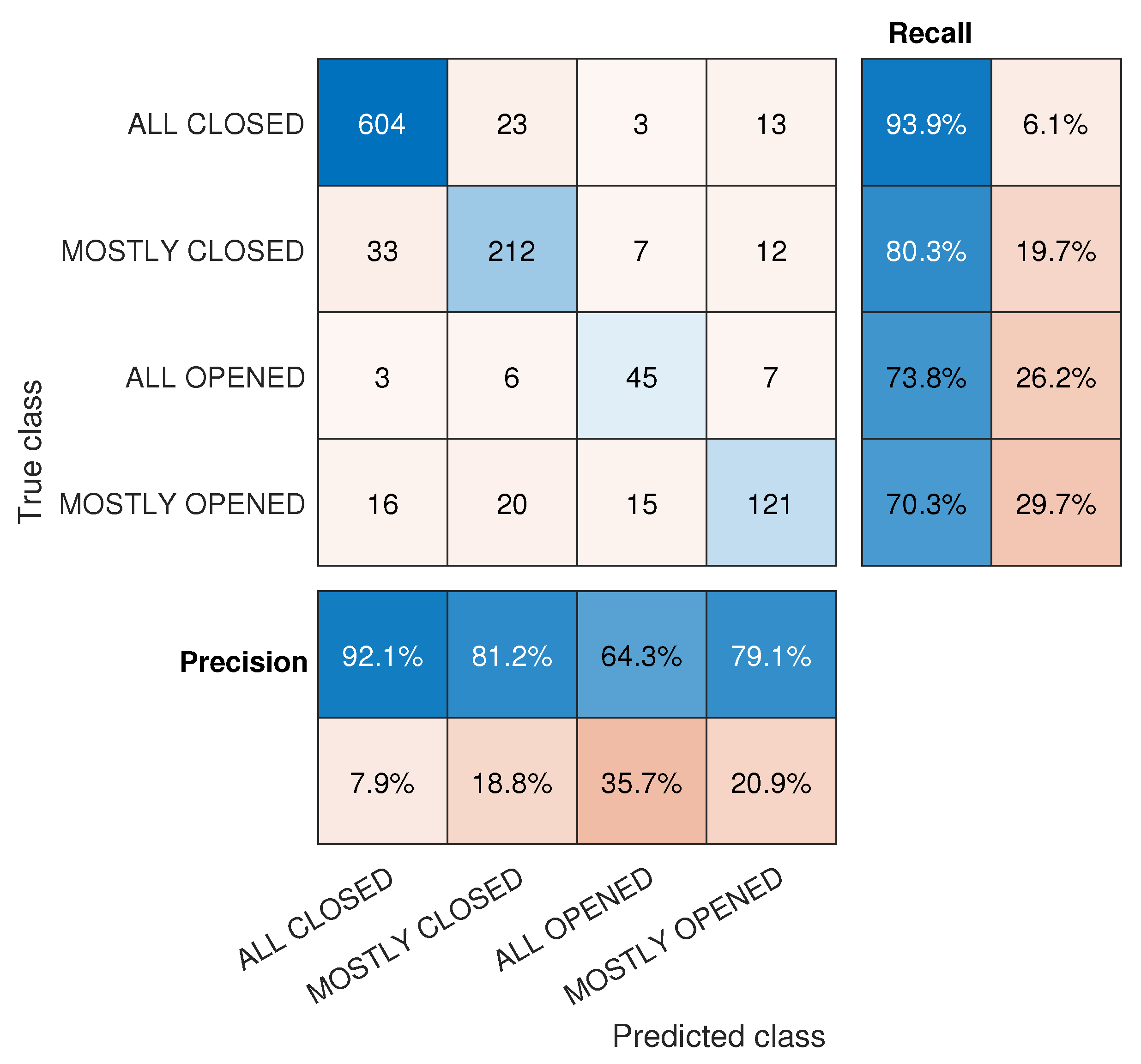
• ALL CLOSED: less than 1 window is opened ($N<1$)
• MOSTLY CLOSED: from 1 to less than 2 windows are opened ($1\le N<2$)
• MOSTLY OPENED: from 2 to less than 4 windows are opened ($2\le N<4$)
• ALL OPENED: 4 windows or more are opened ($N\ge 4$)

The non-environmental parameters’ distribution profiles and the initial statistics of these four groups during the year 2014 are displayed in Figure 2.

Figure 2. Distribution profile of window opening according to the (a) Month, (b) Hour of the day and (c) Day of the week. (d) Statistics for window opening categories.

Firstly, the time series data was divided into sets of consecutive 23 h periods. Next, every 20 first hours of each set were used for training and the other 3 h were used for testing. This results in 7600 h for the training and 1140 h for the testing set (380 sets in total). The reason for choosing a set of 23 h instead of 24 h was that we wanted to achieve an equal distribution of the ‘time of the day’ in both training and testing sets. This can avoid only training on the same specific hours (1 a.m. to 9 p.m., for example, and always testing on the same 3 h in the evening, starting from 10 p.m.).

A Classification Learner Application provided by Matlab software via the Statistics and Machine Learning Toolbox was used to build the classifier. This application trains models to classify data using supervised machine learning. Based on the amount of data that we have, we applied a 10-fold cross validation for the training step, which helps us to limit the overfitting problem. Regarding the setting parameters of our classification model, the Euclidean distance was adopted. Concerning the number of nearest neighbors, for k = 1, we archived the highest accuracy, so the label of a ‘nearest neighbor’ is selected.

3. Results and Discussion

The output of the Classification Learner App shows that a fine k-NN model has been obtained with an accuracy of 92.2%. Using this trained k-NN classifier, we predicted the testing set and compared it to the monitored value, obtaining a value of 86.1% for accuracy. A confusion matrix for this test set is displayed in Figure 3. The highest recall value (true positive rate) is obtained when predicting the ‘ALL CLOSED’ state of the group of windows (93.9%) while the lowest belongs to the ‘MOSTLY OPENED’ label (only 70.3%). Regarding precision values (positive predictive values), the highest value is still obtained by the ‘ALL CLOSED’ state; however, the lowest value corresponds to the ‘ALL CLOSED’ label.

Figure 3. Confusion matrix, precision and recall value (in percentage %) for each label of the test set.

In addition, the statistics for the accuracy of each month, the hour of the day and the day of the week in the testing set are shown in Table 2, Table 3 and Table 4, respectively, where the lower values mostly belong to the summer season (Jun–Sep, except for April), day-time periods (10 a.m.–5 p.m., except for 4 p.m.) and the working day (Mon–Fri), which mostly contains the labels ‘ALL OPENED’ and ‘MOSTLY OPENED’.

Table 2. The statistics for the accuracy of each month in the testing set.

Month	Jan	Feb	Mar	Apr	May	Jun	Jul	Aug	Sep	Oct	Nov	Dec
No. of samples	96	87	96	96	96	93	99	96	93	99	93	96
Accuracy	0.99	0.91	0.85	0.77	0.92	0.83	0.77	0.76	0.71	0.89	0.97	0.98

Table 3. The statistics for the accuracy of each hour of the day in the testing set.

Hour	1st	2nd	3rd	4th	5th	6th	7th	8th	9th	10th	11th	12th
No. of samples	44	44	46	48	49	49	48	48	48	48	48	48
Accuracy	0.91	0.91	0.96	0.96	0.96	0.98	0.98	0.96	0.90	0.67	0.73	0.81
Hour	13th	14th	15th	16th	17th	18th	19th	20th	21st	22nd	23rd	24th
No. of samples	48	48	48	48	48	48	48	48	48	48	47	45
Accuracy	0.85	0.81	0.85	0.90	0.79	0.88	0.81	0.73	0.81	0.85	0.89	0.78

Table 4. The statistics for the accuracy of each day of the week in the testing set.

Day	Mon	Tue	Wed	Thu	Fri	Sat	Sun
No. of samples	162	161	166	162	164	161	164
Accuracy	0.86	0.84	0.83	0.84	0.76	0.96	0.93

Even though the accuracy of the training set is not so high, this is explained by the unequal proportion in each label group, especially the small amount for the ‘ALL OPENED’ label (6.3% as in Figure 2b). Therefore, the model tends to ‘learn well’ with other dominant labels more than with this label. In the future, we can improve this by having an unbiased data set or by providing different weights for each label to penalize misclassification. In addition, the initial set of variables could include the rate of variation of the environmental factors to help improve the performance of the model.

4. Conclusions

In this study, we have obtained a k-NN classification model to predict the opening state for a group of windows in an open-plan office by using both environmental and non-environmental parameters of previous and current samples, including: month, day of the week, time of the day, indoor CO₂ concentration, and both indoor and outdoor temperature and relative humidity. A validation test has been used to compare the outputs of the model and the measured window states observed during the year 2014. We could then use this model by including it in real-time indoor air quality prediction, in order to optimize the action to be taken to reduce the exposure of the occupants.

References

- Indoor Air Division, Office of Atmostpheric and Indoor Air Programs. Congress on Indoor Air Quality: Assessment and Control of Indoor Air Pollution; Technical Report; U.S. Environmental Protection Agency: Washington, DC, USA, 1989.
- Jian, Y.; Guo, Y.; Liu, J.; Bai, Z.; Li, Q. Case study o fwindow opening behavior using field measurement results. Build. Simul. 2011, 4, 107–116. [Google Scholar] [CrossRef]
- Andersen, R.; Fabi, V.; Toftum, J.; Corgnati, S.P.; Olesen, B.W. Window opening behaviour modelled from measurements in Danish dwellings. Build. Environ. 2013, 69, 101–113. [Google Scholar] [CrossRef]
- Yao, M.; Zhao, B. Window opening behavior of occupants in residential buildings in Beijing. Build. Environ. 2017, 124, 441–449. [Google Scholar] [CrossRef]
- D’Oca, S.; Hong, T. A data-mining approach to discover patterns of window opening and closing behavior in offices. Build. Environ. 2014, 82, 726–739. [Google Scholar] [CrossRef] [Green Version]
- Hastie, T.; Tibshirani, R.; Friedman, J. The Elements of Statistical Learning; Springer Series in Statistics; Springer: New York, NY, USA, 2001. [Google Scholar]
- Dai, X.; Liu, J.; Zhang, X. A review of studies applying machine learning models to predict occupancy and window-opening behaviours in smart buildings. Energy Build. 2020, 223, 110–159. [Google Scholar] [CrossRef]
- Ramalho, O.; Ouaret, R.; Ionescu, A.; Le Ponner, E.; Candau, Y. TRIBU–Suivi dynamique en Temps Réel de la qualité de l’air Intérieur dans un environnement de BUreaux. Contributions des sources et Modèle prévisionnel rapport, PRIMEQUAL APR EIAI/projet TRIBU; Technical Report; Scientific and Technical Center for Building (CSTB): Marne-la-Vallée, France, 2016. [Google Scholar]
- Fabi, V.; Andersen, R.; Corgnati, S.; Olesen, B. Occupants’ window opening behaviour: A literature review of factors influencing occupant behaviour and models. Build. Environ. 2012, 58, 188–198. [Google Scholar] [CrossRef]
- Pan, S.; Xiong, Y.; Han, Y.; Zhang, X.; Xia, L.; Wei, S.; Wu, J.; Han, M. A study on influential factors of occupant window-opening behavior in an office building in China. Build. Environ. 2018, 133, 41–50. [Google Scholar] [CrossRef]
- Box, G.; Jenkins, G.M.; Reinsel, G. Time Series Analysis: Forecasting and Control, 3rd ed.; Prentice Hall: Englewood Cliffs, NJ, USA, 1994. [Google Scholar]
Publisher’s Note: MDPI stays neutral with regard to jurisdictional claims in published maps and institutional affiliations. |
© 2021 by the authors. Licensee MDPI, Basel, Switzerland. This article is an open access article distributed under the terms and conditions of the Creative Commons Attribution (CC BY) license (https://creativecommons.org/licenses/by/4.0/).