
Comparative Analysis of Non-Linear GNSS Geodetic Time Series Filtering Techniques: El Hierro Volcanic Process (2010–2014) †


Abstract
:1. Introduction
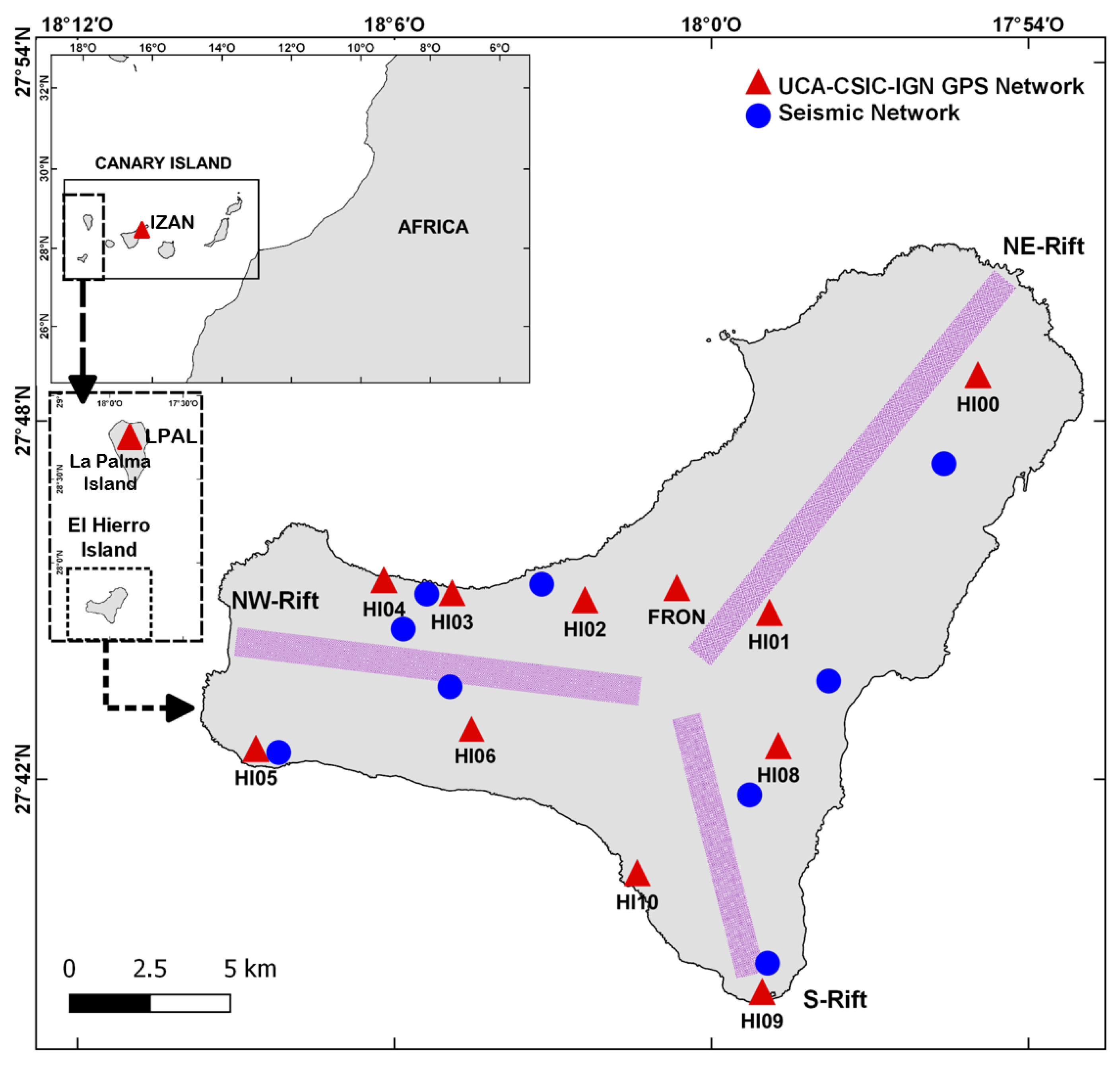
2. Site Description
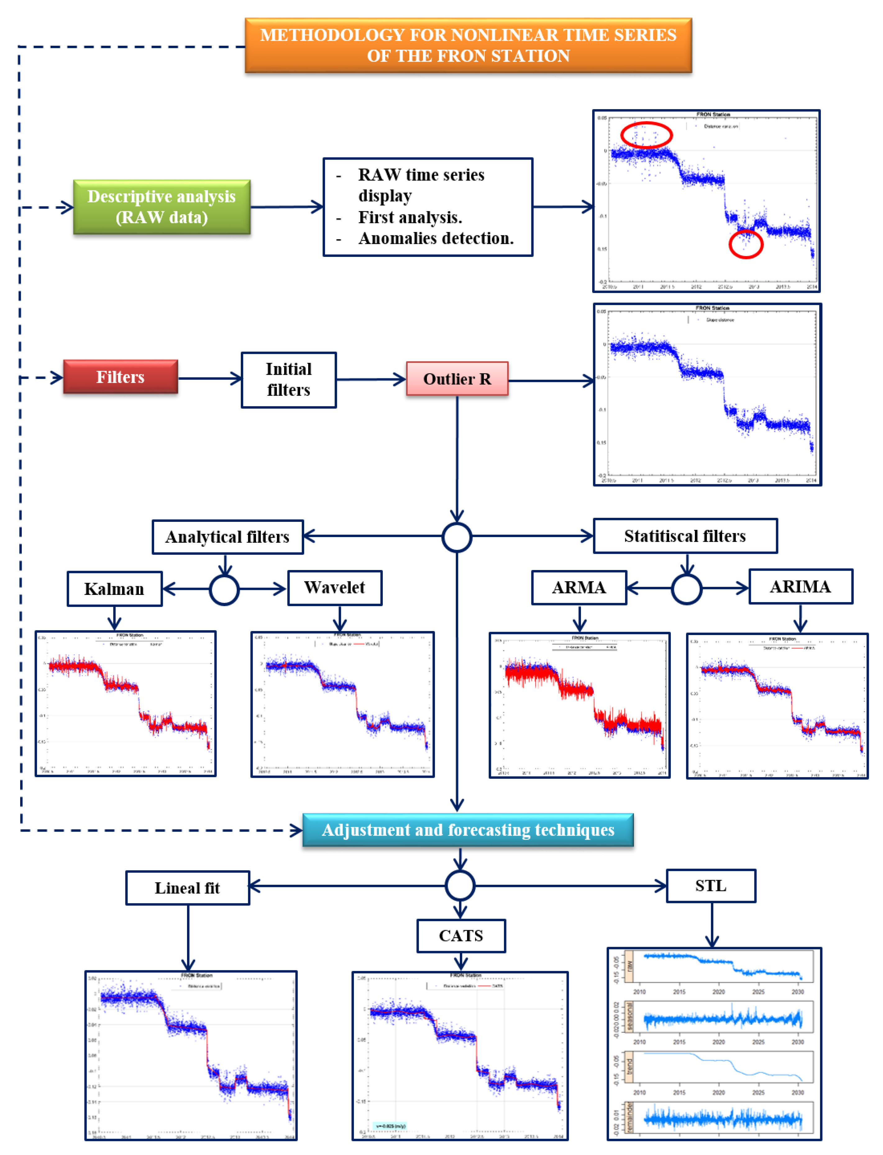
3. Methodology
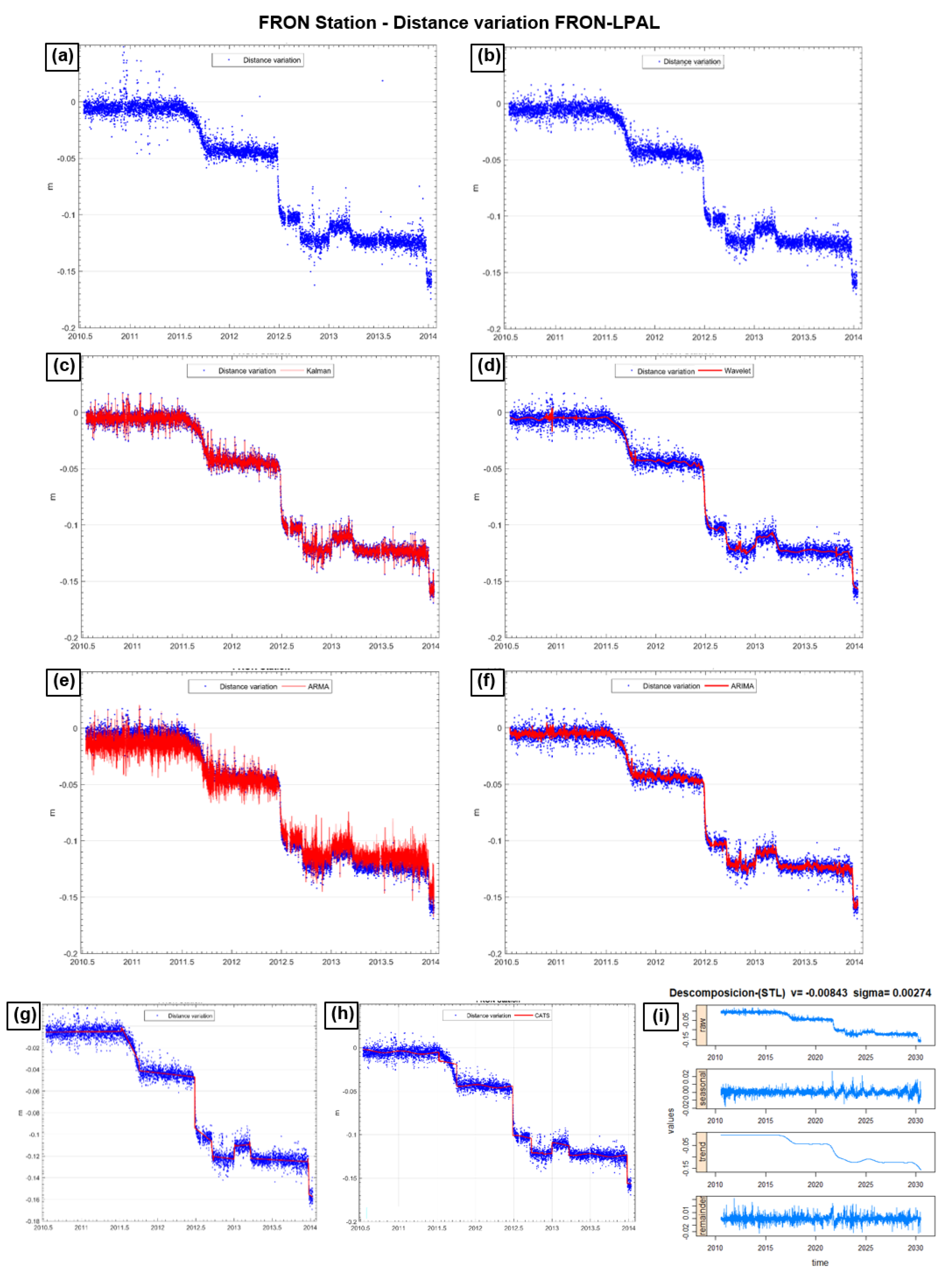
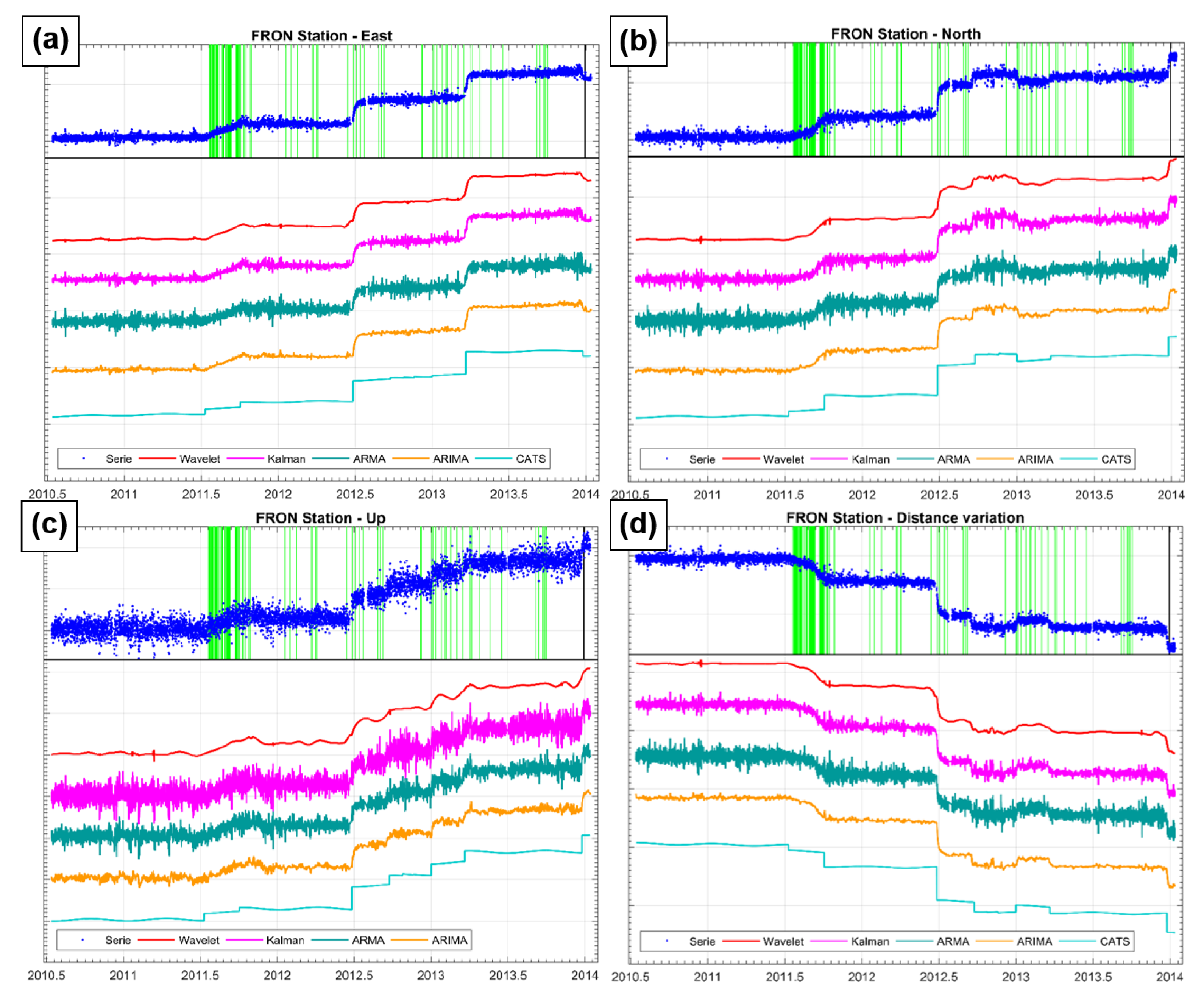
4. Results
Data Availability Statement
Acknowledgments
References
- García, A.; Fernández-Ros, A.; Berrocoso, M.; Marrero, J.M.; Prates, G.; De la Cruz-Reyna, S.; Ortiz, R. Magma displacements under insular volcanic fields, applications to eruption forecasting: El Hierro, Canary Islands, 2011–2013. Geophys. J. Int. 2014, 197, 322–334. [Google Scholar] [CrossRef] [Green Version]
- Prates, G.; García, A.; Fernández-Ros, A.; Marrero, J.M.; Ortiz, R.; Berrocoso, M. Enhancement of sub-daily positioning solutions for surface deformation surveillance at El Hierro volcano (Canary Islands, Spain). Bull. Volcanol. 2013, 75, 724. [Google Scholar] [CrossRef]
- Martín, M.; Rosado, B.; Berrocoso, M. Description of El Hierro volcanic process (2011–2014) from variability analysis of topocentric coordinates obtained by GNSS observations. In Proceedings of the ITISE International work-conference On Time Series, Granada, Spain, 25–27 June 2014; Volume 2, pp. 1293–1298, ISBN 978-84-15814-97-4. [Google Scholar]
- Dach, R.; Hugentobler, U.; Fridez, P.; Meindi, M. Bernese GPS Software ver. 5.0 User Manual; Astronomical Institute, University of Bern: Bern, Switzerland, 2007. [Google Scholar]
- Altamimi, Z.; Collilieux, X.; Metivier, L. ITRF2008: An improved solution of the International Terrestrial Reference Frame. J. Geod. 2011, 85, 457–473. [Google Scholar] [CrossRef] [Green Version]
- Box, G.E.P.; Cox, D.R. An analysis of transformations. J. R. Stat. Soc. 1964, 26, 211–252. [Google Scholar] [CrossRef]
- Larson, K.; Poland, M.; Miklius, A. Volcano monitoring using GPS: Developing data analysis strategies based on the june 2007 Kilauea Volcano intrusion and eruption. J. Geophys. Res. 2010, 115, B07406. [Google Scholar] [CrossRef] [Green Version]
- Rosado, B.; Fernández-Ros, A.; Jiménez, A.; Berrocoso, M. Modelo de deformación horizontal GPS de la región sur de la Península Ibérica y norte de áfrica (SPINA). Boletín Geológico Minero 2017, 128, 141–156. [Google Scholar] [CrossRef]
- Rosado, B.; Fernández-Ros, A.; Berrocoso, M.; Prates, G.; Gárate, J.; De Gil, A.; Geyer, A. Volcano-tectonic dynamics of Deception Island (Antarctica): 27 years of GPS observations (1991–2018). J. Volcanol. Geotherm. Res. 2019, 381, 57–82. [Google Scholar] [CrossRef]
- Box, G.E.P.; Jenkins, F.M. Time Series Analysis: Forecasting and Control, 2nd ed.; Holden-Day: Oakland, CA, USA, 1976. [Google Scholar]
- Williams, S.D.P. CATS: GPS coordinate time series analysis software. GPS Solut. 2008, 12, 147–153. [Google Scholar] [CrossRef]
- Cleveland, R.B.; Cleveland, W.S.; McRae, J.E.; Terpenning, I.J. STL: A seasonal-trend decomposition procedure based on loess. J. Off. Stat. 1990, 6, 3–33. [Google Scholar]


Publisher’s Note: MDPI stays neutral with regard to jurisdictional claims in published maps and institutional affiliations. |
© 2021 by the authors. Licensee MDPI, Basel, Switzerland. This article is an open access article distributed under the terms and conditions of the Creative Commons Attribution (CC BY) license (https://creativecommons.org/licenses/by/4.0/).
Share and Cite
Rosado, B.; Ramírez-Zelaya, J.; Barba, P.; de Gil, A.; Berrocoso, M. Comparative Analysis of Non-Linear GNSS Geodetic Time Series Filtering Techniques: El Hierro Volcanic Process (2010–2014). Eng. Proc. 2021, 5, 23. https://doi.org/10.3390/engproc2021005023
Rosado B, Ramírez-Zelaya J, Barba P, de Gil A, Berrocoso M. Comparative Analysis of Non-Linear GNSS Geodetic Time Series Filtering Techniques: El Hierro Volcanic Process (2010–2014). Engineering Proceedings. 2021; 5(1):23. https://doi.org/10.3390/engproc2021005023
Chicago/Turabian StyleRosado, Belén, Javier Ramírez-Zelaya, Paola Barba, Amós de Gil, and Manuel Berrocoso. 2021. "Comparative Analysis of Non-Linear GNSS Geodetic Time Series Filtering Techniques: El Hierro Volcanic Process (2010–2014)" Engineering Proceedings 5, no. 1: 23. https://doi.org/10.3390/engproc2021005023
APA StyleRosado, B., Ramírez-Zelaya, J., Barba, P., de Gil, A., & Berrocoso, M. (2021). Comparative Analysis of Non-Linear GNSS Geodetic Time Series Filtering Techniques: El Hierro Volcanic Process (2010–2014). Engineering Proceedings, 5(1), 23. https://doi.org/10.3390/engproc2021005023