Robust Underwater Image Classification Using Image Segmentation, CNN, and Dynamic ROI Approximation ^†

Abstract

Finding classified rectangular regions of interest (ROIs) in underwater images is still a challenge, and more so if the images pose low quality with respect to illumination conditions, sharpness, and noise. These ROIs can help humans find relevant regions in the image quickly or they can be used as input for automated structural health monitoring (SHM). This task itself should be conducted automatically, e.g., used for underwater inspection. Underwater inspections of technical structures, e.g., piles of a sea mill energy harvester, typically aim to find material changes in the construction, e.g., rust or pockmark coverage, to make decisions about repair and to assess the operational safety. We propose and evaluate a hybrid approach with segmented classification using small-scaled CNN classifiers (with fewer than 20,000 hyperparameters and 3M unity vector operations) and a reconstruction of labelled ROIs by using an iterative mean and expandable bounding box algorithm. The iterative bounding box algorithm combined with bounding box overlap checking suppressed wrong spurious segment classifications and represented the best and most accurate matching ROI for a specific classification label, e.g., surfaces with pockmark coverage. The overall classification accuracy (true-positive classification) with respect to a single segment is about 70%, but with respect to the iteratively expanded ROI bounding boxes, it is about 90%.

1. Introduction

The underwater inspection of technical structures, e.g., the construction parts of off-shore wind turbines, such as piles, involves the identification of various parts in underwater images. In this work using given videos/pictures, the following things can be included:

• Background with water, bubbles, and fishes, summarised as feature class B;
• Technical structure, e.g., a monopile of a wind turbine, summarised as feature class P;
• Formation of coverage with marine vegetation or organisms on the surface of the structure, summarised as feature class C.

Currently, for the inspection of monopiles, divers have to go underwater. However, even if humans inspect the underwater surfaces (underwater by the diver or remotely), the scenes are cluttered, and the identification of surface coverage is a challenge. Automated visual inspection is desired to reduce maintenance and service times.

Finding classified rectangular regions of interest (ROIs) in underwater images is still a challenge. These ROIs can help humans find relevant regions in the image quickly, or they can be used as input for automated structural health monitoring (SHM). This task itself should be done automatically, e.g., used for underwater inspection. Underwater inspections of technical structures, e.g., piles of a sea mill energy harvester, typically aim to find material changes in the construction, e.g., rust or pockmark coverage, to make decisions about repair and to assess the operational safety.

Images taken from video recordings during diving contain typical changing and highly dynamic underwater scenes consisting of ROIs related to the above-introduced class backgrounds (not relevant), technical construction surfaces, and modified surfaces (rust/pockmark coverage), with the highest relevance.

The aim is the development of an automatic bounded region classifier that is at least able to distinguish between background, construction, and construction + coverage classes. The challenge is the low and varying image quality that typically appears in North and East Sea underwater imaging. The images, typically recorded by a human diver or an AUV, pose low contrast, varying illumination conditions and colours, different viewing angles and spatial orientation and scale, and optical focus issues, overlaid by mud and bubbles (e.g., from the air supply).

We proposed and evaluated a hybrid approach with segmented classification using small-scaled CNN classifiers (with fewer than 10 layers and 100,000 hyperparameters) and a reconstruction of labelled ROIs by using an iterative mean and expandable bounding box algorithm. The iterative bounding box algorithm combined with bounding box overlap checking suppressed wrong spurious segment classifications and represented the best and most accurate matching ROIs for a specific classification label, e.g., surfaces with pockmark coverage. The overall classification accuracy (true-positive classification) with respect to a single segment is about 70%, but with respect to the iteratively expanded ROI bounding boxes, it is about 90%.

The image segment classification and ROI detection algorithms should be capable of being implemented into embedded systems, e.g., directly integrated in camera systems with application-specific co-processor support.

The aim is to achieve an accuracy of at least 85–90% for the predicted images, with a high degree of generalisation and independence from various image and environmental parameters, such as lighting conditions, background colouration, and relevant classification features.

2. Related Work

Overall, there is a lack of freely available image datasets from the underwater area, as discussed by Chongyi Li et al. [1]. A possible image dataset from the underwater area can be found in the Underwater Image Enhancement Benchmark (UIEB DS). These are not specifically technical components, such as ship hulls. Further datasets for underwater images are, for example, the Fish4Knowlege dataset (Fish4Knowledge DS) for the detection and acquisition of underwater targets; underwater images in the SUN dataset for scene recognition and object detection (SUN DS); the MARIS dataset for Autonomous Marine Robotics (MARIS DS); the Sea-thru dataset with 1100 underwater images with range maps; Haze-line dataset with raw images, TIF files, camera calibration files and range maps [2]. Chongyi Li et al., however, criticised that the listed datasets usually have monotonous content, limited scenes, few degradation features and, above all, a lack of reference images. In addition, Mittal et al. criticised the lack of a large-scale dataset, which is why they used data augmentation since it is impossible to train a CNN with scarce data [3]. Another dataset can be found in the ImageNet database, created by Yifeng Xu et al. [4]. The ImageNet 2012 database includes 1000 classes with 15 million labelled high-resolution images (ImageNet DS).

According to Mittal et al. [3] CNNs have already shown better predictive performance than traditional image processing and machine learning methods.

Luo et al. evaluated pre-processing, segmentation, and post-processing for the accurate classification of 108 plankton classes. The authors used greyscale images, which were fraught with noise and unevenness in the greyscale and contrast. In flat fielding, a calculated calibration frame is subtracted from the raw image. They used histogram normalisation to normalise the contrast in each image, which allowed for better segmentation of the ROIs. Extremely noisy images, i.e., those with a signal-to-noise ratio (SNR) below 25, were sorted out. Then they used K-harmonic mean clustering to detect and segment the ROIs.

Deep et al. [5] proposed a CNN model and two CNN + shallow models for the classification of living fish species. In their dataset, most of the images were noise-free but out of focus. Therefore, the images were first pre-processed with an image sharpening method to improve the edges in the images. They used a slightly modified Laplacian kernel, where the sum of all the kernel elements was one instead of zero. This kernel produced a colour image, while the original Laplacian kernel produced a binary image.

3. Image Sets

The image set consisted of different underwater images with a high variance in illumination conditions, spatial orientation, noise (bubbles, blurring), and colour palettes. The images were snapshots taken from videos recorded by a human diver. The images were used for supervised ML requiring explicit labelling. The labelling was done by hand by interactively drawing labelled closed polygon paths and assigning regions of the images to a specific class. There were remaining areas with no/unknown labelling.

4. Methods and Architecture

In addition to the evaluation of suitable algorithms and classification models, this work compared two different software frameworks:

• Native software code using the widely deployed TensorFlow-Keras with GPU support [6];
• Pure JavaScript code using PSciLab with WorkBook and Workshell [6] (processed by a Web browser and node.js), using a customised version of the ConvNet.js trainer for CNNs.

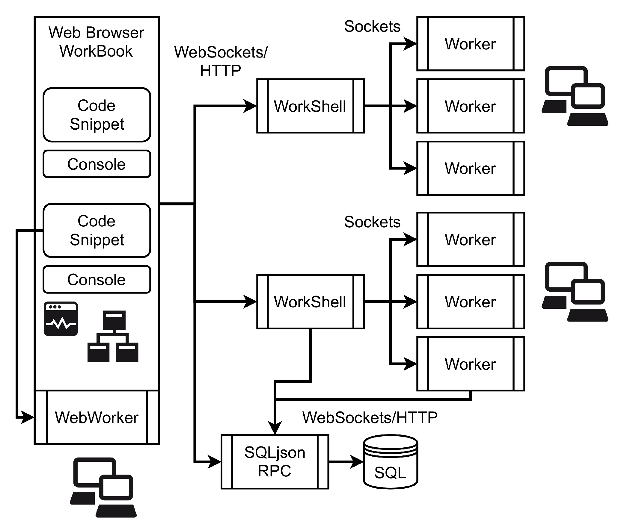
The second framework (see Figure 1) stores all the data in SQL databases and trains the models (JSON format). The SQL databases (SQLite3) can be accessed remotely via an SQLjson Remote Procedure Call (RPC) interface. The TensorFlow framework uses the local filesystem for data storage. For any computer processing, TensorFlow needs a copy of the entire dataset.

Figure 1. Web browser-based software architecture with remote worker processes [1].

Both software frameworks use the same input data and functionally and structurally equivalent CNN architectures.

The dataflow architecture is shown in Figure 2. Starting with the image segmentation process, the segments are the input for the CNN classifier. The output of the segment classifier is used to create a feature map image, that is finally processed by point clustering and bounding box estimation.

Figure 2. Overview of the data flow architecture and the used algorithms.

4.1. Image Segmentation

On the first processing level, the input images were segmented into equally sized sub-images, e.g., RGB segments of 64 × 64 pixels. Each image segment was related to one of the classes σ ∈ {B,P,C} or unknown (U). A conventional CNN with two convolutional layers was used to predict the class σ ∈ {B,P,C} for each single image segment. The CNN was trained with a sub-set of randomly chosen labelled image segments.

4.2. Convolutional Neural Network Architecture

Four different CNN architectures and parameter settings were evaluated and are summarised in Table A1 (Appendix A), assuming segment input site data volumes of 64 × 64 × 3 (RGB) elements (derived from the RGB video images). There were two convolutional layers in all architectures, and the hyperparameter number ranged from 20k to 60k. Both software frameworks used the same CNN architecture and configuration. The smallest CNN model, compared to the largest, required about 1/4 of the unit vector operations and about 1/3 of the hyperparameters that had to be trained.

4.3. Image ROI Classification

The basic algorithm and workflow for automated ROI classification is as follows (see Figure 2):

• Segmentation of each input image with static size segments;
• Parallel prediction of the image segment class by the CNN;
• Creation of a class prediction matrix C^{^} with rows and columns representing the spatial distribution of the image segments in the original input image; the matrix M is considered a point cloud with cartesian point coordinates related to the matrix ⟨row,column⟩ tuple;
• Computation of spatial class element clusters using the DBSCAN algorithm; the parameters 6epsilon and minPoints must be chosen carefully (e.g., ε = 2, minPoints = 5);
• Applying a mean bounding box (MBB) algorithm to the point elements of each cluster computing the mass-centred average bounding box (typically under-sized with respect to the representative points in the clusters);
• Applying an MBB extension iteratively to grow the bounding box but still suppressing spurious (wrong) image segments;
• Remove the small(er) bonding boxes covered by larger bounding boxes (either with a different or the same class) or shrink the overlapping bounding boxes of different classes by priority (shrink the less important regions);
• Mark the original input image with ROI rectangles computed in the previous step.

Iteratively expanded bounding boxes from different classes can overlap, which is an undesired result. To reduce overlapping conflicts, a class priority is introduced. In this work, coverage on construction surfaces had the highest priority to be detected accurately. After the ROI expansion was performed, the overlapping bounding boxes with lower priority classes were shrunk until all overlapping conflicts were resolved.

4.4. Training and Labelling

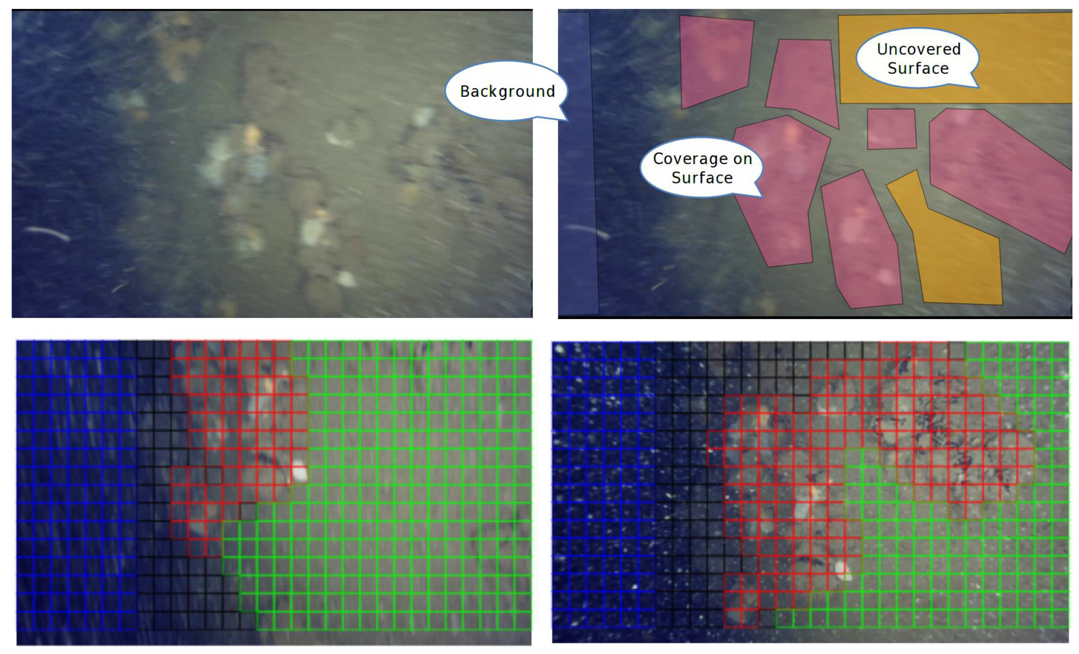
For training, a selected and representative sub-set of images (246 images) were extracted from the diving video. Each image was labelled manually by adding relevant and strong ROI polygons to each image. Based on the labelled and closed polygon paths, each image was segmented with a static segment size. All segments from an image were stored in a SQL database table. With respect to the given image size of 1920 × 1080 pixels and the chosen segment size of 64 × 64 pixels, there were about 120,000 small, labelled image segments. The segment images not covered by any of the labelled polygon paths were automatically marked with the class “Unknown”. Only strong and clearly classifiable regions were created, as shown in Figure 3. The remaining unlabelled regions were not considered for the training process.

Figure 3. Example of the manual labelling of polygon path bounded regions. (Top, Left) Original image. (Top, Right) With labelled polygon regions. (Bottom) Segmented image.

The training process randomly selected a balanced sub-set of the image segments (e.g., 1000) with respect to the class label distribution, i.e., it provided a normal distribution of the class labels among the training and validation datasets. Multiple models were trained in parallel. Each model was trained with a different set of segments and with random initialisation of the model parameters using Monte Carlo simulation.

The TensorFlow framework used an Adam optimiser with a very low learning rate of 0.001. The ConvNetJS CNN framework used an adaptive gradient optimiser with a moderate learning rate of 0.1 and a high momentum of 0.9. Each convolution layer had an l2 regularisation loss with l2 = 0.01 in the TensorFlow framework and l2 = 0.001 in the ConvNetJS framework.

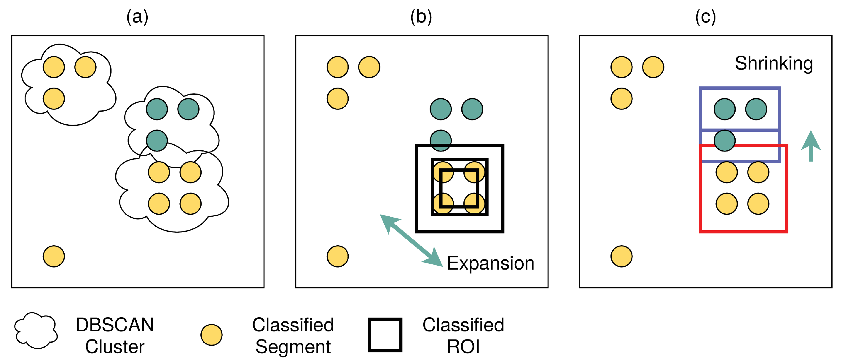
4.5. Mean Bounding Box Algorithm

In this section, the mean bounding box (MBB) algorithm is introduced, applied after the point clustering using the DBSCAN algorithm, shown in Figure 4a. There is a set of class symbols Σ and a class matrix $\widehat{M}$ consisting of elements that label an image segment with a class, so that:

$$\mathrm{\Sigma }=\left\{B,P,C,U\right\}\sigma \in \mathrm{\Sigma }\widehat{M}=\left(\begin{array}{ccc}{\sigma }_{1,1}& \dots & {\sigma }_{1,j}\\ {\sigma }_{2,1}& \dots & {\sigma }_{2,j}\\ \dots & \dots & \dots \\ {\sigma }_{i,1}& \dots & {\sigma }_{i,j}\end{array}\right)$$

(1)

Figure 4. (a) DBSCAN Clustering (b) Iterative bounding box expansion (c) final overlapping conflict shrinking.

The matrix $\widehat{M}$ is flattened to a point cloud list set P = {p_σ}_σ∈Σ. Each class set p contains the matrix positions of the respective elements, i.e., p_σ = {⟨i, j⟩}, with all points classified by the CNN to the same label class σ ∈ Σ.

DBSCAN clustering returns a group list of points that satisfy the clustering conditions, which is one point group list for each label class, as shown in Figure 4a.

$$\begin{array}{l}DBSCAN:P\to \left\{{\left\{p_j\right\}}_j,{\left\{p_k\right\}}_k,{\left\{p_l\right\}}_l,\dots \right\},j\ne k\ne l\\ P:{\left\{p_i\right\}}_i,i=\left\{1,2,3,\dots ,n\right\}\\ p_i=<i,j>\in R^2\end{array}$$

(2)

It was assumed that a cluster contained a majority of correctly classified points (segments), and a minority of scattered wrongly classified points.

The MBB algorithm computes points ⟨x₁, y₁, x₂, y₂⟩ of a bounding box that is centred at the mass-of-centre point c of all points of a cluster, and the outer sides given by the vectorial mean centred position of all points above or below and left or right form the c point, as shown in Algorithm 1 and in Figure 4b.

Algorithm 1. Mean bounding box algorithm applied to a two-dimensional point cloud.

1:  function massOfCentre(points)

2:    pc = {x = 0, y = 0}

3:    ∀p ∈ points do

4:      pc.x: = pc.x + p.x, pc.y: = pc.y + p.y

5:    done

6:    pc: = pc/|points|

7:    return pc

8:  end

9:  function meanBBox(points)

10:    pc = massOfCentre(points)

11:    // Initial bbox around mass-of-centre point

12:    b = {x1 = pc.x, y1 = pc.y, x2 = pc.x, y2 = pc.y}

13:    c = {x1 = 1, y1 = 1, x2 = 1, y2 = 1}

14:    ∀p ∈ points do

15:      // each point extends the bbox

16:      if p.x > pc.x then incr(c.x2), b.x2: = b.x2 + p.x

17:      if p.x < pc.x then incr(c.x1), b.x1: = b.x1 + p.x

18:      if p.y > pc.y then incr(c.y2), b.y2: = b.y2 + p.y

19:      if p.y < pc.y then incr(c.y1), b.y1: = b.y1 + p.y

20:    done

21:    // normalise bbox coordinates

22:    b.x1: = b.x1/c.x1, b.x2: = b.x2/c.x2

23:    b.y1: = b.y1/c.y1, b.y2: = b.y2/c.y2

24:    return b

25:  end

The expansion of a previously computed bounding box is carried out by all the points outside of the current bounding box, performing the next extension iteration (see Figure 4b). Again, spatial position averaging is performed, extending the boundary of the bound box, as shown in Algorithm 2. The expansion is performed iteratively. Each step includes more points but increases the probability that the bound box is over-sized with respect to spurious outlier points that resulted from wrong CNN classifications.

Algorithm 2. Mean bounding box expansion applied to a two-dimensional point cloud and mean bound box.

1:  function meanBBoxExpand(points, b)

2:    pc = massOfCentre(points)

3:    // start with the old bbox

4:    b2 = {x1 = b.x, y1 = b.y, x2 = b.x, y2 = b.y}

5:    c = {x1 = 1, y1 = 1, x2 = 1, y2 = 1}

6:    ∀p ∈ points do

7:      // each point outside the old bbox extends the new bbox

8:      if p.x > b.x then incr(c.x2), b2.x2: = b2.x2 + p.x

9:      if p.x < b.x then incr(c.x1), b2.x1: = b2.x1 + p.x

10:      if p.y > b.y then incr(c.y2), b2.y2: = b2.y2 + p.y

11:      if p.y < b.y then incr(c.y1), b2.y1: = b2.y1 + p.y

12:    done

13:    // normalise bbox coordinates

14:    b2.x1: = b2.x1/c.x1, b2.x2: = b2.x2/c.x2

15:    b2.y1: = b2.y1/c.y1, b2.y2: = b2.y2/c.y2

16:    return b2

17:  end

In the case of high iteration loop values, bounding boxes from different classes can overlap. To reduce overlapping conflicts, a class priority is introduced, layering the class regions by relevance. After the ROI expansion is complete, overlapping bounding boxes with a lower priority are shrunk until all overlapping conflicts are resolved (see Figure 4c). Commonly, more than one side of the bounding box can be shrunk to reduce the overlapping conflict. The possible candidates are evaluated and sorted with respect to the amount of shrinkage on each side. The lowest shrinkage is applied first. If the conflict is not reduced by the selected side shrinking, the next side is shrunk until the conflict (with one or more higher-priority bounding boxes) is reduced, as shown in Figure 4c.

5. Results

The original numeric loss computed from the softmax layer and returned by the trainer is not a measure of the discrete prediction accuracy, i.e., the number of correct and incorrect predicted segment classes, which were achieved after binarisation and the maximum best-of selection. This is an indicator of a low separation margin in the target feature space. 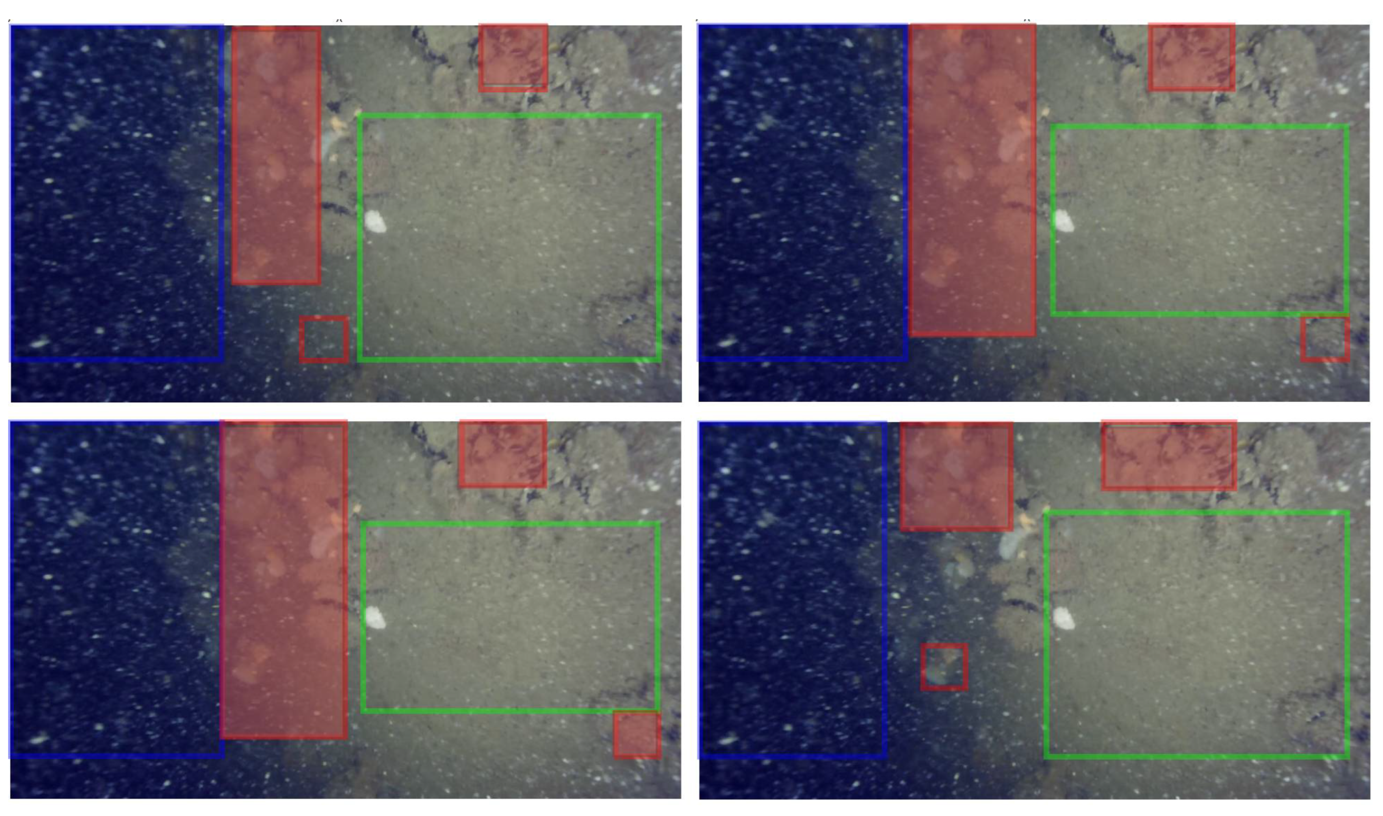There was no significant difference in the accuracy, recall, and precision in the training and test dataset, shown in Table 1. Examples of the classified bounding boxes are shown in Figure 5. Because only the C class (coverage of construction surfaces) is of high relevance (the highest priority), only the particular classification percentages for this class are shown in the last column in Table 1. The average prediction error for all classes was about 10%, with low variance across the different models trained with different sub-sets from the entire dataset, each with different random initialisation. The average errors for specific classes differed significantly. The relevant class C shows a prediction error (¬ C) of about 20%, with respect to the samples, and a high variance across different models. Splitting the prediction accuracy among the tuple true positive (C), false positive (¬ C), true negative (¬ C), and false negative (C) groups, the average TP prediction accuracy was about 80%.

Table 1. Accumulated prediction results for the training and test data and the entire dataset combined, with statistical features of the model ensemble trained in parallel (using different data sub-sets and random initialisation). All errors have a 2σ standard deviation interval, and N = 9000 samples, n = 3000 for each class, using CNN architecture A.

Dataset	Total Error (¬TPC) %	Error (¬TPC)/Class %	Prediction Accuracy/Class C (TP, FP, TN, FN) %
Training	10.6 ± 1.5	5.0 ± 3.4, 6.0 ± 2.8, 21.0 ± 7.1	79.0 ± 7, 4.8 ± 2, 94.7 ± 6.6, 10.5 ± 3.1
Test	11.1 ± 1.8	5.8 ± 2.6, 5.8 ± 3.2, 22.0 ± 8.3	78.0 ± 4.3, 5.1 ± 2.2, 95.1 ± 2.1, 11.0 ± 4.4
All	10.9 ± 1.6	4.2 ± 2.8, 5.9 ± 3.4, 21.7 ± 8	78.4 ± 8, 5.0±2.2, 95.0 ± 2.2, 10.8 ± 4

Figure 5. Classified bounding boxes for one image using four models trained in parallel (same parameters) but with different random initialisation and training data sub-sets (Blue: class background, red: class coverage, green: class-free construction surface).

We obtained the following average statistical measures for the class prediction of the single-image segments:

$$\begin{array}{l}\mathrm{Accuracy}=\frac{\mathrm{TP}+\mathrm{TN}}{\mathrm{TP}+\mathrm{FP}+\mathrm{FN}+\mathrm{TN}}=\{\begin{array}{cc}0.92& \mathrm{train}\\ 0.91& \mathrm{test}\\ 0.92& \mathrm{all}\end{array}\\ \mathrm{Precision}=\frac{\mathrm{TP}}{\mathrm{TP}+\mathrm{FP}}=\{\begin{array}{cc}0.94& \mathrm{train}\\ 0.94& \mathrm{test}\\ 0.94& \mathrm{all}\end{array}\\ \mathrm{Recall}=\frac{\mathrm{TP}}{\mathrm{TP}+\mathrm{FN}}=\{\begin{array}{cc}0.88& \mathrm{train}\\ 0.88& \mathrm{test}\\ 0.88& \mathrm{all}\end{array}\\ \mathrm{Specificity}=\frac{\mathrm{TN}}{\mathrm{TN}+\mathrm{FP}}=\{\begin{array}{cc}0.95& \mathrm{train}\\ 0.95& \mathrm{test}\\ 0.95& \mathrm{all}\end{array}\\ f_1=2\cdot \frac{\mathrm{Recall}\cdot \mathrm{Precision}}{\mathrm{Recall}+\mathrm{Precision}}=\{\begin{array}{cc}0.9& \mathrm{test}\\ 0.9& \mathrm{train}\\ 0.9& \mathrm{all}\end{array}\end{array}$$

(3)

The prediction results for the training and test data do not differ significantly and show similar high statistical measures, which is an indicator of a representative training data sub-set and a sufficiently generalised predictor model.

Considering the bounding box estimator post-processing, the FP rate of the priority class C was nearly zero. The average coverage of the predicted and estimated C area was about 50%, showing an underestimation. The TP rate of class C regions was about 70%.

Typical forward and backward times for the CNN are shown in Table 2. Finally, the different CNN architectures were compared with respect to classification accuracy in Table 3. There was no significant degradation of the classification accuracy observed.

Table 2. Forward and backward (training) times for one 64 × 64 × 3 segment and different CNN architectures (see Figure 3) using the JavaScript ConvNet.js classifier ¹ and TensorFlow (CPU) ².

CNN Architecture	Parameters	Forward Time	Backward Time
A (8/16)	122,587	18 ms 1, 0.5 ms 2	26 ms 1, 1 ms 2
B (4/8)	66,639	8 ms 1	10 ms 1
C (8/8)	104,603	12 ms 1	18 ms 1
D (4/4)	58,047	6 ms 1	8 ms 1

Table 3. Statistical measures of the different CNN model architectures.

CNN	Total Error %	Accu	Prec	Recall	Spec	f1
A (8/16)	11.8	0.909	0.935	0.866	0.947	0.899
B (4/8)	11.8	0.909	0.935	0.866	0.947	0.899
C (8/8)	11.7	0.909	0.936	0.864	0.948	0.899
D (4/4)	12.7	0.900	0.924	0.856	0.938	0.889

In addition to a three-class predictor, a four-class predictor was evaluated, too. An arbitrary unknown class U was added to the class set (i.e., a void class covering “all other” cases). There were no significant improvements in the prediction accuracy of the classes B/P/C observed. A confusion matrix plot of an image segment classification example is shown in Figure 6. Reducing the image segment size by a factor of 2 increased the classification errors significantly, suggesting the 64 × 64 segment size as the lower limit.

Figure 6. Example results (from TensorFlow model) of a four-class predictor with an additional “unknown” class U. (a) 64 × 64 pixel segment size; (b) 32 × 32 pixel segment size.

The increase in accuracy after some image pre-processing techniques (Gaussian blur, rotation) was small and around 1–2%. One major question was the explainability of the CNN classifier and which features of the input image segments were amplified. A first guess was the colour information contained in the image segments. For example, the background was mostly blue or black, and the coverage was mostly white or grey. Therefore, a simple RGB-pixel classifier was applied to each image pixel using a simple fully connected ANN, finally applying the same post-processing algorithms. The results show an average true-positive classification accuracy of about 60%, which is above the guess likelihood (33%), and therefore, the colour feature was still strongly correlated to the classification target label.

Comparing both software frameworks (optimised native code versus virtual machine processing with JavaScript), the overall classification results are similar, and the overall segment classification accuracy was about 90%. The computational time of ConvNet.js was about 50 times higher than that of the CPU-based TensorFlow software. Because the CNN’s complexity was low (fewer than 100,000 parameters distributed over six layers), the data-path parallelisation using single-instruction multiple-data architectures and GGPU co-processors posed no significant speed-up. Control-path parallelisation can be utilised during the training of the model ensemble (maximal speed-up M with M models), and during inference (the maximal speed-up is S, where S is the number of segments per image).

There are different choices for accelerated co-processors, but some of them are limited to TensorFlow only (proprietary interface). The Intel Neural Stick and the Google Coral accelerator are USB dongles with a special TPU chip to perform all tensor calculations. Google Coral works with special pre-compiled TensorFlow Lite networks. The Jetson Nano is the only single-board computer with floating-point GPU acceleration. It supports most models because all frameworks, including TensorFlow, Caffe, PyTorch, YOLO, MXNet, and others, use the CUDA GPU support library at some point. The Raspberry Pi computer can be used with some computational accelerators, such as the Intel Neural Stick2 and the Google Coral USB accelerator. The Google Coral development board has a tensor processing unit (TPU). Jetson Nano has a GPU on board. TensorFlow Lite is compatible with all devices. Originally developed to work in smartphones and other small devices, TensorFlow Lite would never encounter a CUDA GPU. Hence, it does not support CUDA or cuDNN. Thus, the use of TensorFlow Lite on a Jetson Nano is purely based on CPU, not GPU. The Jetson Nano can run TensorFlow models with a GPU on board. However, NVIDIA (Jetson is from NVIDIA) provides TF-TRT on the Jetson Nano. TensorFlow–TensorRT (TF-TRT) is an integration of TensorFlow and TensorRT that leverages inference optimisation on NVIDIA GPUs within the TensorFlow ecosystem.

Table 4 shows a summary of TensorFlow’s performance using widely used image classification networks processed on different hardware devices using accelerators (based on [7]).

Table 4. TensorFlow performance using widely used image classification networks processed on different hardware in image frames per second (FPS) [7].

Model (Input Size)	Raspberry Pi-3/4 (TF-Lite)	Raspberry Pi-3/4 Intel Neural Stick 2	Raspberry Pi-3/4 Google Coral USB	Jetson Nano	Google Coral
EfficientNet-B0 (224 × 224)	14.6–25.8 FPS	95–180 FPS	105–200 FPS	216 FPS	200 FPS
ResNet-50 (244 × 244)	2.4–4.3 FPS	16–60 FPS	10–18.8 FPS	36 FPS	18.8 FPS
MobileNet-v2 (300 × 300)	8.5–15.3 FPS	30 FPS(Pi-3)	46 FPS(Pi-3)	64 FPS	130 FPS
SSD Mobilenet-V2 (300 × 300)	7.3–13 FPS	11–41 FPS	17–55 FPS	39 FPS	48 FPS

6. Conclusions

Although the overall classification accuracy was about 90%, the high variance of the segment prediction results across the differently trained models (with the models all having the same architecture) limited the output quality of the labelled ROI detector, typically resulting in an underestimation of the classified regions and a lack of generalisation. However, the presented static segment prediction with point clustering and iterative selective bounding box approximation with final overlapping conflict reduction was still reliable. Similar to random forest trees, a multi-model prediction with model fusion (e.g., major coverage estimation) is proposed to obtain the best matching bonding boxes for the relevant classes.

The reduction of the CNN complexity with respect to the number of filters and dynamic parameters did not lower the classification accuracy significantly. Although CNNs are less suitable for low-resource embedded systems, CNN architecture D (4/4) could be implemented in embedded camera systems, expecting overall ROI extraction times of about 5 s for one image frame, which is not suitable for real-time operation (maximal latency 100 ms). By using control-path parallelisation to perform the image segment classifications in parallel, the ROI extraction could be reduced to 1 s using generic multi-core CPUs, or 100 ms using FPGA-based co-processors.