Abstract
It is well established that the climate impact of aircraft non-CO2 emissions can be reduced by optimising flight routes to avoid climate-sensitive areas. Little research has been conducted, however, on the effect of residual emissions from nearby aircraft on local atmospheric chemistry and how this may alter the route optimisation process. This paper aims to address these unknowns by observing air traffic data and identifying key hot-spot regions where aircraft plumes are likely to overlap. Providing real-world evidence of these occurrences will serve to justify future atmospheric modelling studies into these effects.
1. Introduction
One-third of aviation’s climate impact is due to carbon dioxide (CO2) emissions. The remaining two-thirds result from the release of non-CO2 emission species such as nitrogen oxides (NOx), water vapour (H2O) and particulate matter. Carbon emissions from aircraft induce warming gradually over their 100–1000 year lifetime directly through the greenhouse effect. Non-CO2 species on the other hand, are much shorter-lived (lifetime on the order of hours to months); however, they exhibit a much stronger heating effect during this time through interaction with chemical and physical processes occurring in the atmosphere.
1.1. Aviation Non-CO2 Climate Impact
Aircraft spend the majority of their flight at cruising altitudes (32,000–42,000 ft), where the air is thin enough to significantly reduce drag, whilst still dense enough to maintain sufficient oxygen flow to the engines. In atmospheric science terminology, this region is known as the Upper Troposphere Lower Stratosphere (UTLS), characterised by its low temperatures, low concentrations of atmospheric trace species and higher radiative efficiencies compared to ground level. Aviation is unique in that it is the only significant source of anthropogenic emissions in the UTLS.
The two most significant contributions to aviation’s high-altitude non-CO2 climate impact are NOx-based ozone production and condensation trails (contrails). Aircraft NOx emissions do not contribute to the greenhouse effect directly; however, they act as a precursor to chemical reactions which produce ozone and deplete methane, both of which are potent greenhouse gases. The warming due to tropospheric ozone production tends to outweigh the cooling due to methane reduction, thus resulting in a net warming effect that constitutes 16% of aviation-related global heating [1].
In the exceptionally cold and moist conditions experienced in the UTLS region, water vapour can condense and freeze around particulate emissions in the aircraft exhaust to form ice crystals. The trail of visible ice crystals that forms behind the aircraft is known as a contrail. Contrails can be short-lived, dissipating over time with a lifetime of seconds to minutes, or they can persist for many hours, growing with time. The criteria for persistent contrail formation is ambient ice supersaturation. When aircraft generate contrails in ice-supersaturated regions (ISSRs), the high ambient humidity facilitates ice crystal growth due to uptake of surrounding atmospheric water vapour. Persistent contrails can spread over hundreds of kilometres and transition to cirrus clouds throughout their evolution, resulting in a substantial man-made increase in high ice cloud coverage globally [2,3].
The radiative properties of contrail ice crystals are such that they are typically more efficient at absorbing and reflecting infrared radiation emitted from the Earth’s surface than they are at scattering inbound solar radiation, resulting in a global heating effect. The warming induced by aviation contrails and contrail cirrus is on the order of 51% of total aviation climate impact [1]. This means that the transient, localised heating effect due to global contrail coverage on a day-to-day basis, is significantly greater than that of all the aircraft CO2 emissions that have accumulated since the beginning of civil aviation [4].
1.2. Mitigating Aviation-Induced Climate Change by Modifying Flight Routes
At cruise altitudes, the degree to which aircraft non-CO2 emissions cause warming or cooling is largely determined by the instantaneous atmospheric conditions (i.e., the local chemical and meteorological situation). The atmospheric state is itself, highly variable with respect to time and location, meaning that the same mass of emissions can have very different climate effects depending on when and where they are released [5]. Climate-optimal routing is an operational mitigation concept proposed to exploit this natural variability in environmental conditions throughout flight. It involves re-routing aircraft to avoid regions of the atmosphere that are particularly sensitive to aircraft emissions. For example, flying around an ISSR region to avoid persistent contrail generation or flying through airspace in which the chemical composition is less conducive to tropospheric ozone formation, as illustrated in Figure 1. Modelling efforts have demonstrated the ability to reduce the climate impact of flying by 10–20% at the expense of only a few percent additional fuel burn [6,7].
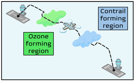
Figure 1.
Conceptual representation of an aircraft trajectory optimised for minimum climate impact.
Further to the notion that natural atmospheric fluxes influence aviation’s non-CO2 climate impact, there is evidence to suggest that artificial perturbations due to emissions from lingering aircraft exhaust plumes may also play a significant role [8,9]. The overlapping of aircraft plumes can locally elevate chemical mixing ratios of key emission species, resulting in chemical saturation effects which are potentially beneficial from a climate change perspective. Firstly, the ability for NOx emissions to produce ozone become hindered once concentrations surpass a threshold concentration. This means that additional NOx input locally will only serve to reduce the NOx-to-ozone conversion efficiency [10]. Persistent contrail formation is also subject to saturation effects. As a persistent contrail grows, it depletes water vapour from the surrounding atmosphere, thus impeding growth of any subsequent contrails formed in the same region [11]. Both these saturation effects lead to a reduction in the resultant non-CO2 climate impact of associated flights compared to the single aircraft scenario. In spite of this, climate-optimal routing studies typically do not consider more than one aircraft, thus neglecting saturation effects caused by residual aircraft emissions. Instead, a range of studies have explored the idea of flying commercial aircraft in formation as a means of reducing both CO2 and non-CO2-related warming.
Formation flight involves flying one or more aircraft, one behind the other at a nominal separation distance of around 1–2 km. The follower aircraft flies in the upwash of the leader aircraft’s wake vortices, which in turn reduces required lift (and hence thrust) for trailing aircraft. As a result, a fuel saving benefit of 5–8% can be achieved [12,13]. The possibility of exploiting chemical saturation effects through controlled plume overlap has also been explored [14,15]. However, no study to date has truly encapsulated the concepts of both climate-optimal routing and formation flight as two parts of the same optimisation problem. Whilst air traffic data have been used in prior studies of aviation emissions [16,17], including modelling of contrail formation [18], this is the first paper to the authors’ knowledge, that will utilise such datasets to analyse the likelihood of aircraft plume overlap in high-density flight scenarios.
2. Methodology
The spatial and temporal distribution of global air traffic is highly inhomogeneous due to variations in passenger demand, safety regulations, airspace organisation and flight route optimisation [19]. Due to the relative unpredictability and non-uniformity in air traffic flows and patterns, modelling and investigation should ideally be based around real-world data. In this paper, historical commercial aircraft trajectory data obtained from the open-source air traffic dataset OpenSky [20] is leveraged to explore how aircraft plumes typically overlap in airspace regions where air traffic denisties are particularly high. The OpenSky Network sources data from Automatic Dependent Surveillance-Broadcast (ADS-B) ground-based receivers, which determine aircraft latitude, longitude and altitude, along with additional measurements such as flight track and ground speed, at a temporal resolution of one second. This dataset is used here to deduce information regarding air traffic flows and airspace density, as well as modelling of aircraft plume intersections, throughout the month of January 2022. All necessary computations were carried out using the Python programming language, coupled with the traffic application programming interface [21] to handle OpenSky data requests, and all plots were generated using Python packages Matplotlib and Cartopy.
In flight air traffic sectors where demand is considerably high or where two or more flight corridors intersect, air traffic can become significantly congested, with airspace capacities often approaching their upper limit [22]. Although undesirable from an air traffic safety and efficiency perspective, it so happens that these regions could provide excellent insight into the real-world practicality of formation flight and controlled plume overlap. Therefore, the first aim of this study was to use OpenSky ADS-B data to locate the highest density flight regions during a typical busy time period. January 2022 was selected, as this represented a point in time where the aviation sector had recovered signfiicantly from the COVID downturn and was prior to the Russian invasion of Ukraine, which further disrupted the air traffic situation considerably. Trajectory data over this month were discretised into 1° longitude × 1° latitude bins, at a typical cruise altitude of 38,000 ft ± 500 ft. The categorised data were then used to construct a global heatmap of mean airspace density for each grid cell. To reduce computational intensity, snapshots of the air traffic situation were taken at the start of every hour, each day of the month.
Following the outcome of the global analysis, two key high-density hot spots were selected for further analysis. The flux densities through the box were calculated for each day and averaged over the whole month to single out the timesteps with the highest average aircraft count. The case study of these two hot spots continued at the subgrid scale through higher resolution observation of trajectories and modelling of their associated exhaust plumes. Dispersion modelling of aircraft plumes has been covered extensively in the literature over the past few decades, with models of varying fidelities becoming widely accepted amongst the community [23]. For this paper, the aim was to select a relatively low fidelity model to track the plume dispersion from OpenSky aircraft trajectories, whilst also being computationally efficient, so that many trajectories could be easily tested. The model used here was that of the Multi-Shell Plume model from Kraabøl et al. [24]. Here, the plume’s horizontal, vertical and skewed standard deviations (, and ) and radii (, ) of the outermost shell were modelled through Equations (1) to (5).
These equations derive from the two-dimensional diffusion equation and hence contain initialised atmospheric parameters according to the assumed turbulent conditions of Durbeck and Gerz [25]: wind shear (s = 0.005 s−1), horizontal (Dh = 16.7 m2 s−1), vertical (Dv = 1.1 m2 s−1) and shear (Ds = 0.5(Dv Dh)2) diffusion coefficients at an arbitrary timestep t. The timestep used in the plume simulations present throughout this paper is 10 s. This means that aircraft positional data were gathered every 10 s, and instances of plume segments were initialised for active aircraft in the grid cell at that particular timestep. For plume instances that already exist, they are expanded at each timestep according to the above equations.
In addition to plume modelling, data were collected on aircraft-to-aircraft information across all flights that traverse through the observed grid cells over the specified timeframe. This includes relative distance, relative track and bearing between aircraft pairs. From this, criteria for scenarios where it was likely that two plume instances would overlap were determined, thus promoting climate-beneficial saturation effects, as elaborated in Section 1. The criteria to be met to achieve successful plume overlap were termed significant plume encounters (SPEs). Based on the E-folding time of NOx and typical contrail growth rates at aircraft cruising altitudes, it was decided that a threshold overlap time for an SPE was around 2 h [26,27]. Thus, the final objective of the study was to determine how many instances of aircraft pairs at each timestep achieved a successful SPE throughout the observed duration.
SPEs were ranked by significance from 1 to 4, as is visually represented in Figure 2. Under assumed plume conditions, horizontal plume radius rh is predicted to reach between 6 and 7 km at the 2 h threshold, whilst rv approaches a mere 75–100 m. SPE ranks were designed in such a way as to capture all instances where plumes from aircraft pairs are likely to overlap prior to the proposed 2 h threshold. SPE1 is classed as any aircraft that is within a 20 km proximity of the baseline aircraft, has a bearing within ±45° of the baseline track and also has a track that is within ±45° of the baseline track. For SPE2, the same rules on relative tracks apply; however, relative distance is between 20 and 50 km. SPE3 counts as any aircraft that is outside of the ±45° boundary, however is within 20 km. Relative headings were neglected here, as any aircraft crossing at such obtuse angles will likely experience plume overlap to some degree. Finally, SPE4 represents any aircraft that does not satisfy any of the other conditions, however is still within a 50 km radius of the baseline aircraft. The ranks were deduced based on relative distance and tracks between all aircraft pairs at every timestep, prioritising tracks over distance. This is because two aircraft flying a similar heading are extremely likely to experience significant and persistent plume overlap even if they are a large distance apart longitudinally. This is because aircraft travel at high speeds and trajectories tend not to deviate too far from their heading during the cruise segment of flight [28].
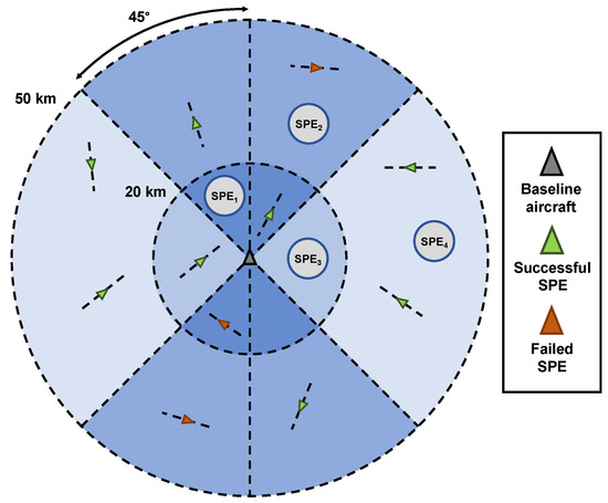
Figure 2.
Schematic drawing of SPE criteria used to deduce plume overlap cases and compare the relative importance of plume intersection events.
3. Results
This study brought to light some interesting findings regarding plume overlap occurrences in real-world air traffic scenarios. Firstly, the results of the global analysis were plotted on a heatmap of mean airspace densities. This was subsequently overlaid onto a world map to allow for visual identification of geographical biases in aviation demand. Figure 3 shows the heatmap with magnification of the two overarching regions with the highest air traffic densities, the East Coast of the United States and Central Europe.
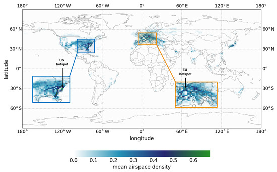
Figure 3.
Global heatmap of mean air traffic density. Snapshots of air traffic data were taken at the first second of every hour throughout January 2022. Mean values are significantly lower than peak values due to large variations in aviation demand throughout the course of each day.
From these magnified regions, the two highest density grid cells were selected for a further subgrid-scale analysis. These were the United States (US) hot spot with a midpoint longitude of −76.5° and latitude of 36.5°, and the European (EU) hot spot at longitude 2.5° and latitude 49.5°. Again, both grid cells are at an altitude of 38,000 ft ± 500 ft. Before conducting the high resolution subgrid-scale study, it was first necessary to cherry-pick a suitable time interval to investigate, as running plume simulations over the entire month period was too computationally expensive. Instead, using trajectory data resampled at 1 min intervals, the average aircraft count for each hour of the day was calculated over the whole month, for each hot spot grid cell. The results can be seen in Figure 4.
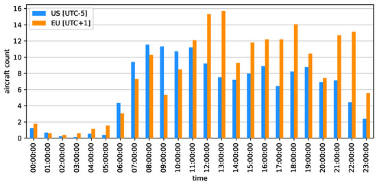
Figure 4.
Temporal variation in average aircraft count for the two hot spots for each hour of the day, over all days in January 2022.
The US hot spot has notably less peaky data than the EU alternative; however, it peaks earlier, at 08:00:00 EST (UTC-5), whereas the EU peaks at 13:00:00 CEST (UTC+1). The absolute highest count for the US was 26 aircraft on 24 January 2022 at 08:00:00 EST. For the EU, it was 31 aircraft on 29 January 2022 at 13:00:00 CEST. Using these peak dates and times, a detailed plume analysis was then performed, using the plume modelling approach outlined in Section 2. For each hot spot, the air traffic situation over three hours (peak time ± 1 h) was observed.
For both hot spots over the specified duration, data were collected on distances, headings and bearings between aircraft pairs at each timestep (every 10 s). Plume instances are modelled as circles on a 2D map, meaning it is not possible to visually distinguish altitude differences and vertical plume extent. Altitude was left out of the plots because aircraft in cruise rarely tend to deviate far from their designated flight level.
Table 1 presents numerical results from the subgrid-scale plume study, which collected data from 2114 aircraft pair instances for the US hot spot, and 2443 for the EU hot spot. For each, some key aircraft pair information was computed, and the SPE tests were conducted for each data point, including a test for no SPE occurrence at all (i.e., the data points which do not meet the SPE criteria).

Table 1.
Key information regarding significant plume encounters for both hot spots.
4. Discussion
From the results presented, it can be deduced that there may well be huge potential to exploit chemical saturation effects to reduce the non-CO2 warming from aviation. Intersecting plumes in high-density airspace regions can lead to a diminishing influence of both NOx-based effects and persistent contrail growth. In this study, high-density hot spots were first investigated through a global heatmap analysis (Figure 3). This plot of “mean airspace density”, combined with the peak aircraft counts per hour, derived in Figure 4, exemplify the temporal inhomogeneity of air traffic distribution, typically seen at aircraft cruising altitudes. Even for the highest density grid cells, the maximum average aircraft density is just above 0.6 aircraft per grid volume. Comparing this to a maximum flux of 31 aircraft traversing through the EU hot spot at its peak hour, shows that traffic patterns can be highly nonlinear and unpredictable.
In the plume plots of Figure 5a,b, it is evident that despite the EU hot spot having a higher number of aircraft pairings over the 3 h period, the traffic in the US hot spot seems to be following a much more organised track structure. This has a large effect on the ability to achieve plume overlap, as can be seen in the results in Table 1. Even though the EU has 329 more instances of aircraft pairings recorded, the vast majority of its data points did not record an SPE occurrence (81.4%). The US, on the other hand, achieved a 42% SPE success rate despite having a smaller aircraft count. As a result, this suggests that the US hot spot could have served as a better candidate for controlled plume overlap and that there are many other factors in play that may determine the effectiveness of this method (e.g., airspace complexity, temporal distribution, airspace organisation, etc.).
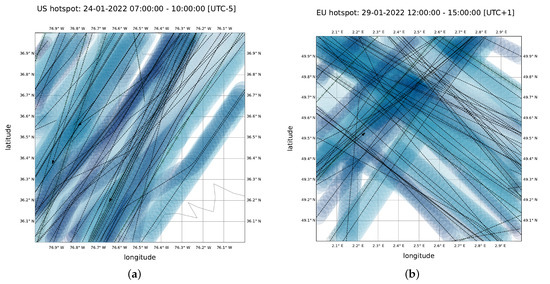
Figure 5.
Plume modelling simulation for high density hot spots: (a) US hot spot; (b) EU hot spot.
5. Limitations
Whilst ADS-B trajectories enable aircraft exhaust plume intersections to be identified, there are limitations regarding usage for exhaust plume modelling. Firstly, identification of exhaust plume interactions is limited to global regions with ADS-B OpenSky Network ground receiver coverage; therefore, global estimates of aircraft exhaust plume intersections are not currently feasible. This limitation includes areas where sustained exhaust plume interactions are likely, such as oceanic crossings, particularly along the North Atlantic Flight Corridor where densities are typically high [8].
Another significant limitation of relying solely on ADS-B derived-trajectories is the lack of meteorological information. The accurate modelling of exhaust plumes and contrails will of course be reliant on the pre-existing atmospheric conditions, along with an estimated plume drift due to wind conditions [18]. Consequently, the study presented in this paper has assumed that the plume follows the aircraft ground track. Future work could employ the meteorological information supplied my Mode-S data or alternative approaches for estimating wind conditions via Mode-S data [29] for the aircraft identified with plume intersections within the ADS-B dataset to generate improved plume modelling. When considering 3D plume modelling, further investigations into variations of reported GPS and barometric altitudes of operational aircraft is required, especially for the discrete ‘steps’ in aircraft altitude observed within ADS-B trajectories.
A final limitation with respect to considering solely ADS-B trajectories for identifying aircraft exhaust plume intersections is a result of the plume size and dispersion being related to aircraft operational parameters, including aircraft size (i.e., mass) and flying speeds. Both of these parameters will impact the engine exhaust flow and the wake generated by the aircraft, which are expected to impact the size and dispersion of the aircraft exhaust plume. Future work would aim to address this by coupling ADS-B trajectories with aircraft characteristics prior to conducting plume modelling runs.
6. Conclusions
In this paper, open-source air traffic data has been utilised to gain insight into the potential for plume intersections in high-density flight regions, such as flight corridors and over mainland continental areas. A global analysis of mean air traffic densities was initially carried out to identify potential candidate regions which could be tested for formation flight and controlled plume overlap. A higher resolution study was then performed on two regions which exhibited exceptionally high airspace densities throughout the observed time period. This localised study shed light on some nuances in the way air traffic is typically distributed and the effect that can have on the likelihood of significant plume intersections. Further work would ideally take this a step further by carrying out a more in-depth analysis of the atmospheric chemistry and climate response to this change in operations. For now, however, this paper has drawn attention to the possibilities. It is now up to the field to build a more concrete modelling and analysis framework to increase scientific understanding of the benefits and unintended consequences of implementation, and finally, to bring these concepts closer to fruition in commercial aviation.
Author Contributions
Conceptualization, K.N.T. and J.H.; methodology, K.N.T., J.H. and S.R.; software, K.N.T. and S.R.; formal analysis, K.N.T.; investigation, K.N.T. and J.H.; data curation, K.N.T.; writing—original draft preparation, K.N.T.; writing—review and editing, J.H.; visualization, K.N.T. All authors have read and agreed to the published version of the manuscript.
Funding
This research was funded by the Engineering and Physical Sciences Research Council (EPSRC) as part of a Doctoral Training Partnership (DTP).
Institutional Review Board Statement
Not applicable.
Informed Consent Statement
Not applicable.
Data Availability Statement
Historic air traffic data from the OpenSky Network.
Acknowledgments
The authors would like to thank Steve Bullock, Mark Lowenberg, Md. Anwar Khan and Dudley Shallcross of the University of Bristol for their enlightening discussions regarding the wider context of this work. We also appreciate the help of Joe Dunlop, for bringing key elements of this study to our attention at a crucial time.
Conflicts of Interest
The authors declare no conflict of interest.
References
- Lee, D.S.; Fahey, D.W.; Skowron, A.; Allen, M.R.; Burkhardt, U.; Chen, Q.; Doherty, S.J.; Freeman, S.; Forster, P.M.; Fuglestvedt, J.; et al. The contribution of global aviation to anthropogenic climate forcing for 2000 to 2018. Atmos. Environ. 2021, 244, 117834. [Google Scholar] [CrossRef] [PubMed]
- Kärcher, B. Formation and radiative forcing of contrail cirrus. Nat. Commun. 2018, 9, 1824. [Google Scholar] [CrossRef] [PubMed]
- Schumann, U.; Heymsfield, A. On the Life Cycle of Individual Contrails and Contrail Cirrus. Meteorol. Monogr. 2017, 58, 3.1–3.24. [Google Scholar] [CrossRef]
- Burkhardt, U.; Kärcher, B. Global radiative forcing from contrail cirrus. Nat. Clim. Chang. 2011, 1, 54–58. [Google Scholar] [CrossRef]
- Matthes, S.; Lührs, B.; Dahlmann, K.; Grewe, V.; Linke, F.; Yin, F.; Klingaman, E.; Shine, K.P. Climate-optimized trajectories and robust mitigation potential: Flying ATM4E. Aerospace 2020, 7, 156. [Google Scholar] [CrossRef]
- Niklaß, M.; Lührs, B.; Grewe, V.; Dahlmann, K.; Luchkova, T.; Linke, F.; Gollnick, V. Potential to reduce the climate impact of aviation by climate restricted airspaces. Transp. Policy 2019, 83, 102–110. [Google Scholar] [CrossRef]
- Matthes, S.; Lim, L.; Burkhardt, U.; Dahlmann, K.; Dietmüller, S.; Grewe, V.; Haslerud, A.S.; Hendricks, J.; Owen, B.; Pitari, G.; et al. Mitigation of Non-CO2 Aviation’s Climate Impact by Changing Cruise Altitudes. Aerospace 2021, 8, 36. [Google Scholar] [CrossRef]
- Schlager, H.; Konopka, P.; Schulte, P.; Schumann, U.; Ziereis, H.; Arnold, F.; Klemm, M.; Hagen, D.E.; Whitefield, P.D.; Ovarlez, J. In situ observations of air traffic emission signatures in the North Atlantic flight corridor. J. Geophys. Res. 1997, 102, 10739–10750. [Google Scholar] [CrossRef]
- Jaeglé, L.; Jacob, D.J.; Brune, W.H.; Faloona, I.C.; Tan, D.; Kondo, Y.; Sachse, G.W.; Anderson, B.; Gregory, G.L.; Vay, S.; et al. Ozone production in the upper troposphere and the influence of aircraft during SONEX: Approach of NOx-saturated conditions. Geophys. Res. Lett. 1999, 26, 3081–3084. [Google Scholar] [CrossRef]
- Jenkin, M.; Clemitshaw, K. Ozone and other secondary photochemical pollutants: Chemical processes governing their formation in the planetary boundary layer. Atmos. Environ. 2002, 1, 285–338. [Google Scholar]
- Unterstrasser, S.; Gierens, K. Numerical simulations of contrail-to-cirrus transition—Part 1: An extensive parametric study. Atm. Chem. Phys. 2010, 10, 2017–2036. [Google Scholar] [CrossRef]
- Xu, J.; Ning, A.; Bower, G.; Kroo, I. Aircraft Route Optimization for Formation Flight. J. Aircr. 2014, 51, 490–501. [Google Scholar] [CrossRef]
- Bangash, Z.; Sanchez, R.; Ahmed, A.; Khan, M.J. Aerodynamics of formation flight. J. Aircr. 2004, 43, 907–912. [Google Scholar] [CrossRef]
- Dahlmann, K.; Matthes, S.; Yamashita, H.; Unterstrasser, S.; Grewe, V.; Marks, T. Assessing the climate impact of formation flights. Aerospace 2020, 7, 172. [Google Scholar] [CrossRef]
- Marks, T.; Dahlmann, K.; Grewe, V.; Gollnick, V.; Linke, F.; Matthes, S.; Stumpf, E.; Swaid, M.; Unterstrasser, S.; Yamashita, H.; et al. Climate Impact Mitigation Potential of Formation Flight. Aerospace 2021, 8, 14. [Google Scholar] [CrossRef]
- Filippone, A.; Parkes, B.; Bojdo, N.; Kelly, T. Prediction of aircraft engine emissions using ADS-B flight data. Aeronaut. J. 2021, 125, 988–1012. [Google Scholar] [CrossRef]
- Sun, J.; Basora, L.; Olive, X.; Strohmeier, M.; Schäfer, M.; Martinovic, I.; Lenders, V. OpenSky Report 2022: Evaluating Aviation Emissions Using Crowdsourced Open Flight Data. In Proceedings of the 2022 IEEE/AIAA 41st Digital Avionics Systems Conference (DASC), Portsmouth, VA, USA, 18–22 September 2022. [Google Scholar]
- Gruber, S.; Unterstrasser, S.; Bechtold, J.; Vogel, H.; Jung, M.; Pak, H.; Vogel, B. Contrails and their impact on shortwave radiation and photovoltaic power production—A regional model study. Atmos. Chem. Phys. 2018, 18, 6393–6411. [Google Scholar] [CrossRef]
- Gössling, S.; Humpe, A. The global scale, distribution and growth of aviation: Implications for climate change. Glob. Environ. Chang. 2020, 65, 102194. [Google Scholar] [CrossRef]
- Schäfer, M.; Strohmeier, M.; Lenders, V.; Martinovic, I.; Wilhelm, M. Bringing Up OpenSky: A Large-scale ADS-B Sensor Network for Research. In Proceedings of the 13th IEEE/ACM International Symposium on Information Processing in Sensor Networks (IPSN), Berlin, Germany, 15–17 April 2014; pp. 83–94. [Google Scholar]
- Olive, X. traffic, a toolbox for processing and analysing air traffic data. J. Open Source Softw. 2019, 4, 1518. [Google Scholar] [CrossRef]
- Odoni, A. The Flow Management Problem in Air Traffic Control. In Flow Control of Congested Networks; Springer: Capri, Italy, 1987; pp. 269–288. [Google Scholar]
- Paoli, R.; Cariolle, D.; Sausen, R. Review of effective emissions modeling and computation. Geosci. Model Dev. 2011, 4, 643–667. [Google Scholar] [CrossRef]
- Kraabøl, A.G.; Konopka, P.; Stordal, F.; Schlager, H. Modelling chemistry in aircraft plumes 1: Comparison with observations and evaluation of a layered approach. Atmos. Environ. 2000, 34, 3939–3950. [Google Scholar] [CrossRef][Green Version]
- Dürbeck, T.; Gerz, T. Dispersion of aircraft exhausts in the free atmosphere. J. Geophys. Res. Atmos. 1996, 101, 26007–26015. [Google Scholar] [CrossRef]
- Shallcross, D.; (University of Bristol, Bristol, UK). Personal Communication, 2022.
- Kraabøl, A.G.; Stordal, F. Modelling chemistry in aircraft plumes 2: The chemical conversion of NOx to reservoir species under different conditions. Atmos. Environ. 2000, 34, 3951–3962. [Google Scholar] [CrossRef]
- Tait, K.N.; Khan, M.A.H.; Bullock, S.; Lowenberg, M.H.; Shallcross, D.E. Aircraft Emissions, Their Plume-Scale Effects, and the Spatio-Temporal Sensitivity of the Atmospheric Response: A Review. Aerospace 2022, 9, 355. [Google Scholar] [CrossRef]
- Sun, J.; Vû, H.; Ellerbroek, J.; Hoekstra, J.M. Weather field reconstruction using aircraft surveillance data and a novel meteo-particle model. PLoS ONE 2018, 13, 10. [Google Scholar] [CrossRef]


Disclaimer/Publisher’s Note: The statements, opinions and data contained in all publications are solely those of the individual author(s) and contributor(s) and not of MDPI and/or the editor(s). MDPI and/or the editor(s) disclaim responsibility for any injury to people or property resulting from any ideas, methods, instructions or products referred to in the content. |
© 2022 by the authors. Licensee MDPI, Basel, Switzerland. This article is an open access article distributed under the terms and conditions of the Creative Commons Attribution (CC BY) license (https://creativecommons.org/licenses/by/4.0/).