Abstract
A crank press is converted into a smart fatigue testing machine for 3-point bending of polymer matrix composite specimens. The press is retrofitted with a load cell base for work holding, which monitors the bending force applied by the ram, a cycle counter recording the number of loading cycles, and a camera recording snapshots of the specimen area where failure is expected. A convolutional and Resnet neural networks are trained to recognize failure as an area of color change in camera images. Signal drop on the load cell signals failure onset, thus triggering monitoring by the camera and execution of the neural network. Acceptable proof-of-concept results encourage further automation of the setup.
1. Introduction
Fatigue testing machines are fundamental tools in material science and engineering, providing insights into durability, reliability, and safety of structural components under cyclic loading. Fatigue testing machines have undergone significant advancements in recent years, driven by both technological innovation and the growing demands of modern materials engineering. The core function of these machines is to replicate the cyclic stresses that materials experience during service, enabling the evaluation of fatigue life under controlled laboratory conditions. Commercial fatigue testers offer advanced functionality and precision but remain very costly and often impractical for academic or low-budget applications.
Several studies have explored alternative fatigue machines aimed at cost reduction and design simplification. Vincent et al. [1] proposed low-cost fatigue rigs, though with limitations in accuracy and automation. Kulkarni et al. [2] developed bending fatigue setups for composite materials, while McAlorum et al. [3] presented machines adaptable for long-duration or multi-purpose testing. Hadi et al. [4] and Nagabhooshanam et al. [5] applied similar approaches to specific material classes.
A central challenge in fatigue testing is the detection of damage or failure initiation in the shape of cracks, delaminations, etc., depending on the material and propagation. Traditional observation methods are labor-intensive, motivating the integration of computer vision and machine learning. Wang et al. [6] introduced convolutional neural networks (CNNs) for crack recognition, while Singh and Desai [7] as well as Singh et al. [8] evaluated pre-trained CNNs and data augmentation strategies. Comparative studies by Park et al. [9], Weimer et al. [10], and Xu et al. [11] examined CNN architectures for defect detection, emphasizing trade-offs between accuracy, computational cost, and dataset size.
The present work repurposes a mechanical press into a fatigue testing machine, upgrading it with load cells, automated cycle counting, and neural-network-based failure detection, as a step toward fully automated S–N diagram generation for diverse materials. Section 2 summarizes the state-of-the-art in fatigue testing machines. Section 3 presents the modifications accomplished in the mechanical press at hand to transform it to a fatigue testing machine. Section 4 outlines the details of the neural network used to detect failure status in the specimen undergoing testing. Section 5 presents indicative results of sample tests and briefly discusses them. Section 6 summarizes conclusions and gives a short outlook.
2. Fatigue Testing Machines
Depending on the application, various loading modes are employed, including uniaxial tension-compression, torsion, and bending. Bending fatigue, in particular, introduces alternating tensile and compressive stresses across the specimen cross-section. Advanced systems also support multiaxial and variable amplitude loadings, more accurately simulating complex service conditions [12].
The structural design and actuation of fatigue testing machines vary depending on required load capacity and testing frequency. Servo-hydraulic systems remain the industry standard for high-force applications, offering precise control over load and waveform, albeit with limitations in operating frequency. Electromechanical systems, utilizing ball screws or linear actuators, are gaining popularity due to their straightforward operation and lower maintenance, despite the associated moderate load capacity. For high-frequency application (very high cycle fatigue (VHCF) testing) ultrasonic systems operating near 20 kHz are employed, requiring specialized specimen geometries and thermal management [13].
Sensorization plays a pivotal role in modern fatigue testing machines. Load cells, Linear Variable Differential Transformer (LVDTs), extensometers, strain gauges, and digital image correlation systems provide comprehensive monitoring of force, displacement, and strain. In high-frequency tests, additional instrumentation such as thermal sensors and accelerometers is required to monitor temperature rise and dynamic response. Under the Industry 4.0 paradigm, fatigue machines aim at integration with advanced digital infrastructure, enabling real-time data acquisition, predictive analytics, and machine learning-based diagnostics. These systems often incorporate virtual sensing, where physical measurements are combined with finite-element models to estimate internal stresses and strains at unmeasured locations, thus reducing sensor requirements and enhancing system insight [14]. Thus, integration of digital twins, cloud-based analytics, and AI-driven failure prediction models represents a promising direction in fatigue testing machines.
3. Press Repurposing into a Fatigue Testing Machine
A single action eccentric press with a maximum stroke of 150 mm was converted into a smart fatigue testing machine in bending mode; see Figure 1. The bending force is applied by the press’s ram to the specimen held on a special jig on the press’s table.
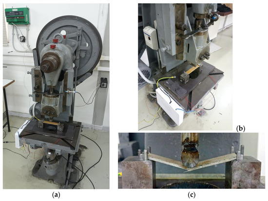
Figure 1.
The repurposed machine. (a) General view; (b) loading table; (c) load application.
The stroke frequency was originally not adjustable; thus, an inverter (CDSTM75, Control Techniques, Newtown, United Kingdom) was used to modify the rotational speed of the press’s motor. In addition, a counter of the number of strokes (fatigue cycles) was necessary. This was implemented by a Hall sensor actuated at the ram’s top position and sending the appropriate signal to an Arduino microcontroller, where an interrupt function was applied to count the number of signal transitions from low to high. Initially, the corresponding signal was distorted due to noise; therefore, a 1st order filter was implemented to solve this issue.
The work holding jig consists of a SverkerTM steel plate (Uddeholms AB, Hagfors, Sweden), measuring 250 × 150 × 20 mm and bearing a hole 100 mm in diameter, to allow observation of the specimen by a camera from below, i.e., opposite to the ram. The plate was clamped on the press table having four low-cost SparkfunTM SEN-10245 (SparkFun Electronics, Niwot, CO, USA) load cells, each one consisting of a half Wheatstone bridge and measuring load independently. Thus, the total load applied by the ram is the sum of all four loads measured. Each load cell has a capacity of 500 N, its excitation voltage is < 10 V and its output sensitivity is 1 mV/V. An HX711TM load cell amplifier (SparkFun Electronics, Niwot, CO, USA) was connected to the microcontroller. Since the load cells are low-cost, they needed in situ calibration by sequentially applying 5 known weights (5, 10, 20, 30, 40 kg) and measuring the resulting voltage to calculate by best fit the calibration factor.
The specimen rests on two blocks with a span of 100 mm with ground round filet edges of radius 5 mm. The specimen is held in place by two side pins on each block, restricting its movement back and forth, and one back gauge on each block restricting its left–right movement; see Figure 1c. The blocks’ edge filets act in fact as rollers but the friction on their contact with the specimen does restrict the latter’s unwanted movement. The load is applied by a steel cylinder of diameter 25 mm attached to the ram. Note that although standard ASTM D-7774 [15] dictates alternating displacements upwards and downwards with respect to the flat shape of the specimen, so far, only the downwards displacement was implemented to keep jig design simple.
A DFKTM ΜΚU130-10x22 camera (The Imaging Source, Bremen, Germany) was positioned under the press table for recording failure on the underside of the specimen; see Figure 2.
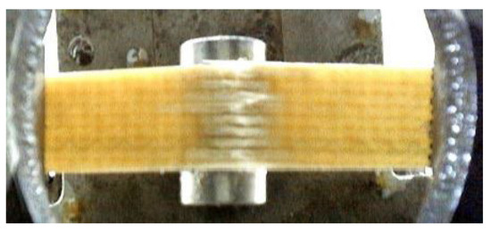
Figure 2.
Camera snapshot of failed specimen.
Ambient (artificial light) of the room was adequate so that no special light was used, at least in this proof-of-concept approach. The camera image undergoes background clipping in real time to isolate the specimen area where failure is expected to emerge. Images were taken by the camera, not on-the-fly but after stopping the fatigue testing, i.e., when an appropriate signal is given. This may correspond to the predetermined number of cycles (strokes) or after the load cells indicated a drop in load, i.e., failure onset. The signal is given by the microcontroller to a relay that stops the inverter. As soon as the image from the camera is taken, it is passed to the neural network, which generates an output regarding possible failure. The neural network workflow is executed in PythonTM 3.7.16 code on a PC. The code, once the verdict is reached, sends a signal through the serial port to the microcontroller and this, in turn, signals the relay to start the inverter again. The process is repeated until either a predetermined number of cycles has been completed or no substantial load is recorded, i.e., the specimen fully failed.
4. Neural Network for Specimen Failure Detection
The dataset for training the neural network to recognize failure was constructed by artificially over-bending specimens on a vice in the laboratory. This was necessary because fatigue-induced failure was too time-consuming. Failure in Glass Fibre Reinforced Plastic (GFRP) specimens is typically manifested as a differently colored region in the specimen’s bottom surface subjected to tension while bending. Indeed, there was no visual difference between specimens that failed under fatigue and under static loading; see Figure 3.
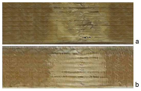
Figure 3.
Plan view of failed specimens under (a) static loading; (b) fatigue loading.
Initially, color photos at a reduced resolution of 200 × 200 pixels of 65 healthy and 65 damaged specimens were gathered. They were transformed to black and white to reduce the file size. Each photo was pre-processed by cropping based on the k-means clustering algorithm.
The dataset obtained by direct phοtography was too small for neural network training. Therefore, augmentation was applied to finally obtain 585 healthy and 585 damaged specimen photos by varying brightness and contrast of the original ones.
From each subset, i.e., healthy and damaged specimens, 45 photos were used for testing, while the remaining 540 were used for training. By randomly changing selection of the testing and training photos, 10 different training datasets and corresponding 10 testing datasets were obtained. Each dataset was used to train a convolutional network and subsequently test it. For comparison, a pre-trained ResNet-50 network was tested with the same testing datasets.
The CNN included two convolutional layers. The first layer has 64 3 × 3 kernels and the second has 256 kernels. Activation function was ReLU and max pooling of dimensions 2 × 2 was employed. The rate employed at the dropout layer was 40%. The output layer consisted of one neuron with sigmoid activation function, i.e., possible values 0 or 1 corresponding to failure or health. Early stopping technique was applied for network training.
The second network is a pre-trained binary classification ResNet-50 network [16], with learning rate 0.0001, early stopping, dropout rate of 30%, and ReLU activation function (sigmoid at the output).
Accuracy of testing for the ten datasets is presented in Figure 4 and is considered (just) promising. In some cases (e.g., 7 and 8) accuracy reached 100%, but in others, such as 1, 4, and 6, it was much lower. The mean accuracy attained was 79% for the CNN and 86% for the ResNet-59. ResNet-50 is generally better; however its lower-than-expected performance may be attributed to the low resolution of the images fed to it. On the other hand, the CNN might improve given a larger number of training images and a higher resolution at the same time. Training of the CNN takes 1–5 min depending on the computer used. However, once trained, image recognition is executed in tens of a second on either network.
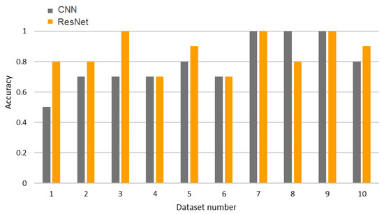
Figure 4.
Testing accuracy for the 10 different subsets of the augmented dataset.
5. Results and Discussion
Indicative fatigue tests for three specimens denoted as A, B, and C are documented in Figure 5. Specimen dimensions were 130 × 25 × 3.3 mm.
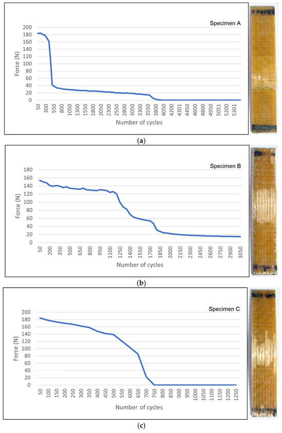
Figure 5.
Indicative specimen cases tested to failure.
Specimens consist of modified acrylic resin (Ashland Modar 835S, Ashland, Wilmington, DE, USA) plus fire retardant additive (ATH 901, Sibelco, Antwerp, Belgium), with five layers of glass fiber reinforcements, namely (a) 64003 Ahlstrom [±0°/+45°/+90°/−45°] quadriaxial reinforcements and (b) chopped strand mat M501 in the [64003–M501–64003–M501–64003] symmetric configuration.
The specimens were made by hand layup, thus having internal flaws expected to lead to failure. Fatigue tests were conducted at 32 mm maximum displacement at the center of the specimen.
Results are recorded in vector form, i.e., [number of cycles, load, failure flag] in csv format, from which appropriate plots can be made; see Figure 5.
The three specimens A, B, and C failed according to low-cycle fatigue mechanisms. They exhibit similar maximum loads at the beginning of the fatigue test: 180 N, 155 N and 185 N, respectively. However, they subsequently exhibit diverting behavior as bending cycles accumulate. In Specimen A, the force drops drastically at 550 cycles, followed by a low force plateau for about 3000 more cycles before force zeroing. Specimen B exhibits a load turning point at 1200 cycles, followed by a gradual, i.e., not steep, drop to a low value within the next 600 cycles and a low plateau afterward. Specimen C exhibits a moderate decrease in force, up to 500 cycles, followed by a much sharper decrease in the next 250 cycles, reaching zero force at 750 cycles.
Referring to diagrams in Figure 5 the difference in load vs. number of cycles is classic for hand-laid GFRP. Even when the first-cycle load is the same, as, for instance, in Specimens A and C, manufacturing and local-damage differences can produce totally different fatigue behaviors, ranging from sudden brittle collapse to slow progressive degradation. A critical defect such as a large void, delamination, ply wrinkle, resin-starved area, bonded inclusion, or local fiber break can turn into an unstable crack, which, upon reaching critical size, leads to a quick failure of the remaining cross-section. On the other hand, distributed damage, such as matrix microcracking, small delaminations, fiber–matrix debonding, and fiber pull-out, may accumulate gradually, reducing stiffness and load capacity over many cycles until final failure. Note that no further investigation was made to discover the causes of the different failure behavior of specimens A, B, and C, because the aim of this work was to show the functionality of the machine developed and not to investigate failure mechanisms of GFRP specimens.
6. Conclusions and Further Work
The machine that was converted from a simple mechanical press proved to be functional and adequately controlled by low-cost equipment. A low-cost microcontroller proved adequate for the relatively simple workflow and not so demanding response time to the events involved. However, low-cost load cells and noise may jeopardize reliability of measurements.
The machine is simple to use, since the operator only needs to adjust the stroke on the ram and execute the control software through the corresponding user-friendly interface. However, a PC is needed for executing the Neural Network in parallel to the execution of the control program on the microcontroller. This undermines compactness of the system.
ResNet50, primarily, but also CNNs attain promising performance in specimen failure determination from photos with relatively few training examples. CNN architecture design is best to start with a few hidden layers and proceed with an increase only, if necessary, for reasons of fast response. It might benefit from larger datasets and more ingenuous augmentation of cases, e.g., using Generative Adversarial Networks.
In the future, firstly, video will replace photos to avoid interruptions in testing process. Photo resolution will be increased in ANN training and operation. Then, ANN will be upgraded to quantify the extent of failed specimen damage. An upgraded microcontroller capable of executing the trained neural network will be sought in order to improve compactness and self-sufficiency of the system.
Author Contributions
Conceptualization, G.-C.V.; methodology, N.D.; software, N.D. and E.S.; validation, N.D., E.T. and E.S.; investigation, N.D.; resources, E.T.; data curation, N.D.; writing—original draft preparation, N.D.; writing—review and editing, G.-C.V.; supervision, G.-C.V. and E.S. All authors have read and agreed to the published version of the manuscript.
Funding
This research received no external funding.
Institutional Review Board Statement
Not applicable.
Informed Consent Statement
Not applicable.
Data Availability Statement
The raw data supporting the conclusions of this article will be made available by the authors on request.
Acknowledgments
Konstantinos Kerasiotis of the Manufacturing Technology Laboratory, National Technical University of Athens is gratefully acknowledged for helping with equipment setup.
Conflicts of Interest
The authors declare no conflicts of interest.
References
- Vincent, M.K.; Varghese, V.; Sukumaran, S. Fabrication and analysis of fatigue testing machine. Int. J. Eng. Sci. 2016, 5, 15–19. [Google Scholar]
- Kulkarni, P.V.; Sawant, P.J.; Kulkarni, V.V. Design and development of plane bending fatigue testing machine for composite material. Mater. Today Proc. 2018, 5, 11563–11568. [Google Scholar] [CrossRef]
- McAlorum, J.; Rubert, T.; Fusiek, G.; Niewczas, P.; Zorzi, G. Design and demonstration of a low-cost small-scale fatigue testing machine for multi-purpose testing of materials, sensors and structures. Machines 2018, 6, 30. [Google Scholar] [CrossRef]
- Hadi, S.; Murdani, A.; Sudarmadji, S.; Artiko, A. Testing of the ability of fatigue test machine prototype and fatigue test for nylon and cast iron specimens. IOP Conf. Ser. Mater. Sci. Eng. 2020, 732, 012094. [Google Scholar] [CrossRef]
- Nagabhooshanam, N.; Baskar, S.; Nagarajan, P.K. Design and fabrication of fatigue test rig and preliminary investigation on flax composite beam. Mater. Today Proc. 2018, 5, 11771–11779. [Google Scholar] [CrossRef]
- Wang, S.Y.; Zhang, Y.; Zhou, Y.; Wei, Z.; Ding, Y.; Li, J. A computer vision based machine learning approach for fatigue crack initiation sites recognition. Comput. Mater. Sci. 2020, 171, 109259. [Google Scholar] [CrossRef]
- Singh, S.A.; Desai, K.A. Automated surface defect detection framework using machine vision and convolutional neural networks. J. Intell. Manuf. 2023, 34, 1995–2011. [Google Scholar] [CrossRef]
- Singh, S.A.; Kumar, A.S.; Desai, K.A. Comparative assessment of common pre-trained CNNs for vision-based surface defect detection of machined components. Expert Syst. Appl. 2023, 218, 119623. [Google Scholar] [CrossRef]
- Park, J.-K.; Kwon, S.; Hyub Park, J.; Kang, J. Machine learning-based imaging system for surface defect inspection. Int. J. Precis. Eng. Manuf.-Green Technol. 2016, 3, 303–310. [Google Scholar] [CrossRef]
- Weimer, D.; Scholz-Reiter, B.; Shpitalni, M. Design of deep convolutional neural network architectures for automated feature extraction in industrial inspection. CIRP Ann. 2016, 65, 417–420. [Google Scholar] [CrossRef]
- Xu, L.; Lv, X.; Deng, Y.; Li, X. A weakly supervised surface defect detection based on convolutional neural network. IEEE Access 2020, 8, 42285–42296. [Google Scholar] [CrossRef]
- Marques, J.M.; Benasciutti, D.; Niesłony, A.; Slavič, J. An overview of fatigue testing systems for metals under uniaxial and multiaxial random loadings. Metals 2021, 11, 447. [Google Scholar] [CrossRef]
- Macek, W.; Zawiślak, S.; Deptuła, A.; Ulewic, R. Fatigue testing machines and apparatus. Zesz. Nauk. Qual. Prod. Improv. 2019, 1, 80–108. [Google Scholar] [CrossRef]
- Mora, B.; Basurko, J.; Leturiondo, U.; Albizuri, J. Strain Virtual Sensing Applied to Industrial Presses for Fatigue Monitoring. Sensors 2024, 24, 3354. [Google Scholar] [CrossRef] [PubMed]
- ASTM D-7774-12; Standard Test Method for Flexural Fatigue Properties of Plastics. ASTM International: West Conshohocken, PA, USA, 2022.
- He, K.; Zhang, X.; Ren, S.; Sun, J. Deep residual learning for image recognition. In Proceedings of the IEEE Conference on Computer Vision and Pattern Recognition, Las Vegas, NV, USA, 27–30 June 2016; pp. 770–778. [Google Scholar]


Disclaimer/Publisher’s Note: The statements, opinions and data contained in all publications are solely those of the individual author(s) and contributor(s) and not of MDPI and/or the editor(s). MDPI and/or the editor(s) disclaim responsibility for any injury to people or property resulting from any ideas, methods, instructions or products referred to in the content. |
© 2025 by the authors. Licensee MDPI, Basel, Switzerland. This article is an open access article distributed under the terms and conditions of the Creative Commons Attribution (CC BY) license.