Hysteresis in Precipitation–Dissolution Cycling of Hydrides in Zirconium Alloys Is an Illusion

Abstract

Experimental results are compiled to show apparent hysteresis seen in hydride thermal precipitation–dissolution cycling in zirconium alloys using X-ray diffraction, dynamic elastic modulus techniques, and differential scanning calorimetry (DSC). Gibbs’ phase rule is used to justify a description of a stable hydride in the H-Zr system in terms of a control volume with a hydride at its core, surrounded by a stress gradient that produces a stabilizing gradient of hydrogen in the solution. The conditions for a stable hydride are derived when the flux of hydrogen in solid solution is zero. DSC heat flow curves are analyzed with a thermodynamic model that predicts concentrations of hydrogen in a solution during temperature cycling and a description of experimental results that show how concentrations evolve at a constant temperature to the same final state when cycling is paused, from which hysteresis is deemed an illusion. The control volume is supported by previous energy calculations, performed with density functional theory. Implications of replacing the order parameter for phase field methods with the gradient of the yield stress are discussed. A practical method for forming a stable hydride is presented.

1. Introduction

Hydrogen is the most abundant element in the universe: it is everywhere. Hydrogen is in all metals used by engineers. Hydrogen can change the properties of metals. Hydrogen can be in a solid solution where it changes the lattice parameters, and it can interact with crystal imperfections, including dislocations and grain boundaries, and form brittle hydrides that can lead to failures of engineering structures. Hydrogen will be used for fuel cells and, inevitably, metals will be used to store, transport, and contain hydrogen, and hydrogen ingress is bound to happen. In metal alloys, hydrogen atoms are the fastest diffusing species because of their small mass, so the effects of hydrogen on properties can often be quickly noticed.

Temperature cycling can cause hydrides to precipitate and dissolve in zirconium alloys. These processes of precipitation and dissolution are much more complicated in solid solutions than in liquid solutions. When a precipitate forms in a liquid solution—for example, sugar crystals forming in water with cooling—the water is displaced by the volume of the crystals and the incidental hydrostatic stress caused by this displacement on the crystals is negligible. In a solid solution, the volume of the hydrides is larger than the volume of zirconium from which the hydrides form. The metal atoms are displaced elastically and plastically by the formation of the hydride. The subsequent hydrostatic stress is not negligible. The result is that during cooling, hydrides dissolve and precipitate, and during heating, hydrides precipitate and dissolve. Stable hydrides are surrounded by a cloud of hydrogen in the solution that relieves the strain caused by the hydride when it forms. This cloud forms over time and stabilizes the hydride over tens of degrees Celsius above and below the formation temperature. Dissolution and precipitation both happen during cooling and heating, in part because hydrides are moving outside of their temperature stability ranges [1].

Figure 1 shows heat flow measurements for three successive differential scanning calorimetry (DSC) precipitation–dissolution cycles for hydrogen in zirconium. The deviations from a parallelogram are differential heat flows associated with hydrides precipitating and dissolving in a zirconium sample when compared with a similar reference sample without hydrogen.

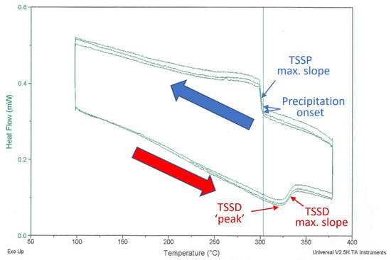
Figure 1. DSC endothermic and exothermic heat flow for a 134 mg sample cut from a Zr coupon. The temperature was scanned at ±1 °C/min between 100 °C and 380 °C; shown here are three successive cycles after the initial ‘conditioning’ cycle. The determined maximum slope temperatures are 331 °C (endothermic) and 300 °C (exothermic). The difference between the maximum slope temperatures is conventionally interpreted as hysteresis. The vertical line shows the onset precipitation temperature is 304 °C. The red arrow corresponds to the endothermic scan during heating and the blue arrow corresponds to the exothermic scan during cooling.

The ‘precipitation-onset’ temperature at 304 °C is the first ‘thermal’ indication of hydride formation during cooling from a temperature at which there are no stable hydrides. The heat flow rises with further cooling because hydride formation is exothermic. The maximum-slope temperature, labelled TSSP in Figure 1, is often quoted for DSC measurements. Hydride dissolution is indicated by the lower portion of the heat flow curve. In this case, the direction of the deviation from the reference changes, because dissolution is endothermic. When heated, the TSSD maximum slope temperature is often quoted. The difference between the TSSD and TSSP maximum slope temperatures is the hysteresis.

Since 1964, it has been common to associate ‘hysteresis’ with separate concentration versus temperature plots determined when heating and cooling hydrides in zirconium alloys [2]. The total concentration of hydrogen in a sample is the dependent variable, and these maximum slope temperatures of precipitation and dissolution are independent variables. The common interpretation is that these curves represent unique concentrations of hydrogen in the solution at various temperatures during precipitation and dissolution, as described in the caption of Figure 2. These concentration–temperature curves are called TSSP and TSSD where the letters stand for Terminal Solid Solubility for Precipitation and Dissolution, respectively, as shown in Figure 2 for Zr-2.5Nb alloy. Terminal solid solubility (TSS) is synonymous with the equilibrium solvus between hydrogen in solid solution and hydrogen in hydride form. Although TSS is part of the label for these two curves, strictly, there is only one TSS, or one solvus, according to Gibbs’ phase rule [3].

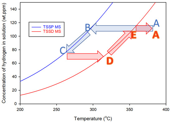
Figure 2. Standard TSS curves for Zr-2.5Nb containing hydrogen, determined from the maximum slope (MS) temperatures of the exothermic and endothermic DSC heat flows that define TSSP and TSSD, respectively ([4] Equations (D.2-2) and (D.2-1)). An example of a conventional precipitation–dissolution cycle is shown by the arrows. Cooling from Point A, the concentration of hydrogen in the solution does not change as the TSSD curve is crossed, staying constant until Point B. With further cooling, the concentration follows the TSSP curve until Point C. Heating does not change the concentration until Point D and with further heating, the concentration follows the TSSD curve until Point E, where all the hydrogen is back in the solution. The apparent hysteresis is approximately 60 °C, and the ratio of the TSSP and TSSD concentrations is about 1.9 at 300 °C.

The term hysteresis might have originated from comparisons with stress–strain curves loaded past the elastic limit that show non-linear behaviour associated with plastic work in the form of dislocations. The stress–strain curve seen when loading is not the same as the stress–strain curve seen when unloading, because the dislocations formed during loading cause a residual offset strain that persists during unloading. It is argued that the plastic work introduced in each cycle is responsible for the hysteresis seen in hydride precipitation and dissolution cycling [5]. The inference is that precipitating hydrides push against the metal lattice, forming dislocations, and indeed, there are micrographs that show hydrides surrounded by dislocations: see Figure 3 for an example.

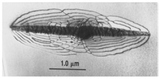
Figure 3. A transmission electron micrograph of a γ-hydride in zirconium, surrounded by dislocations [Reprinted/adapted with permission fromS.A. Aldridge].

TSSP and TSSD provide calibration curves that associate precipitation and dissolution temperatures with total concentrations that are assumed to be everywhere, the same as in the metal. During heating and cooling, the concentration of hydrogen in the solution presumably follows these solvi curves that define the hysteresis. If taken literally, this interpretation leads to a paradox when samples are heated and cooled to the same temperature and connected so that hydrogen can flow between samples. At equilibrium, the concentrations cannot be different, yet the two ‘equilibrium’ solvi curves suggest they are, and hydrogen in the solution should flow from the high-concentration cooled sample to the lower-concentration heated sample. In this case, the final concentration of hydrogen in the solution everywhere in both samples will be the TSSD value, which is contrary to the notion of hysteresis.

The purpose of this paper is to show how concentrations of hydrogen in a solid solution change with temperature during hydride precipitation and dissolution cycling by reconciling conflicting interpretations of observations of X-ray diffraction, dynamic elastic modulus (internal friction), and differential scanning calorimetry (DSC). DSC heat flow curves are confounded by athermal hydrides that do not present measurable thermal signals when they precipitate. These DSC curves are analyzed with a thermodynamic model that predicts concentrations of hydrogen in the solution during temperature cycling and a description that shows how concentrations evolve at a constant temperature when cycling is paused. The interpretation developed in this paper is based on the concept of a control volume, defined in accordance with Gibbs’ phase rule, and by a stabilizing cloud of hydrogen in a solution (reminiscent of Cottrell atmospheres of carbon in steels), which forms over time around a hydride when it precipitates. Practical applications will be discussed.

2. Two Solvi Violate Gibbs’ Phase Rule

Gibbs’ phase rule is a foundational principle in material thermodynamics that is used to describe the nature of phase boundaries on phase diagrams [3]. The phase boundary in question is the α-phase/(α-phase + γ-hydride): see Figure 4.

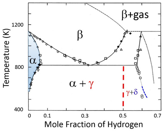
Figure 4. Zirconium–hydrogen phase diagram based on [6,7]. The solvus is the equilibrium boundary that separates the shaded region (α-phase), where saturated hydrogen is in a solid solution in the α-zirconium lattice, and the region (α-phase + γ-hydride), where ZrH hydrides have precipitated in the lattice. The β and β + gas regions indicate bcc zirconium with dissolved hydrogen and coexistence with hydrogen gas, respectively. At higher hydrogen contents, the γ-hydride + δ-hydride two-phase region are shown.

The state of each phase can be derived from the Gibbs–Duhem equation, which shows the necessary relationship between simultaneous changes in chemical potential, μ, temperature, T, and pressure, p. For the α phase,

$${\displaystyle \sum _{i=1}^{\mathrm{C}}{N}_i}\mathrm{d}{\mu }_i=-S\mathrm{d}T+V\mathrm{d}p$$

(1)

where C is the number of different components in the system, S is the entropy, and V is the partial molar volume of hydrogen in the solution.

There are four variables that need to be assigned to completely determine the state of the H-Zr system: two chemical potentials, μ, for the two components (i.e., one potential for hydrogen in a solution in the α-phase, and one for hydrogen in a solution in equilibrium with hydride, or hydrogen in hydride.); and two additional variables, one for temperature and a second for pressure. At equilibrium, the values of each of these variables are constant throughout the system. In general, the number of variables that need to be assigned is C + 2.

There are two phases (P = 2) for the H-Zr phase system and thus, two Gibbs–Duhem equations: one for hydrogen in the solution in the α-phase, Equation (1), and one for hydrogen in contact with hydride.

The number of independent variables is equal to the number of variables that need to be assigned, C + 2, minus the number of equations, P, i.e., the number of unknowns minus the number of equations, to give Gibbs’ phase rule:

$$\mathrm{F}=\mathrm{C}+2-\mathrm{P}$$

(2)

The degrees of freedom, F, is the number of variables in the system whose values may be freely chosen by the experimentalist and must be chosen before the system is in a deterministic state. The system of equations is under-determined.

For practical application of the phase rule to hydrogen in zirconium, the phase rule is modified to account for the oxide barrier on the metal that stops hydrogen ingress and egress. Thus, there is no partial pressure of hydrogen gas in equilibrium with hydrogen in the metal. The pressure of the atmosphere is negligible compared with the hydrostatic pressure imposed on the hydrogen by the metal (0.1 kPa compared with hundreds of MPa) and it does not change significantly when hydrides precipitate or dissolve; there is no effect or change in external pressure.

The implication of the arguments made in the preceding paragraph is that the number of degrees of freedom is reduced by one because the Vdp term in Equation (1) is zero: the pressure/stress does not change. The number of variables that need to be assigned is C + 1 and the ‘reduced’ phase rule, sometimes called the condensed phase rule, becomes the following:

$$\mathrm{F}=\mathrm{C}+1-\mathrm{P}$$

(3)

For the H-Zr system where there are two components and two phases, F = 1.

The phase diagram shows regions of different phases. The phase boundaries denote equilibrium conditions between phases that can be calculated with the Gibbs’ energy:

$$\mathrm{d}G=V\mathrm{d}p-S\mathrm{d}T+{\displaystyle \sum _i{\mu }_i}\mathrm{d}{N}_i$$

(4)

for a closed system where the entropy and volume of the system are assumed to be constant. At equilibrium, the energy is a minimum, so dG equals zero and Vdp is zero for the reasons provided above. The variables that remain are temperature and concentration. If one of temperature or concentration is given, the other is determined. Thus, phase diagrams for two-component, two-phase systems consist of temperature–concentration graphs, as shown in Figure 4, for example.

For the H-Zr α-phase/(α-phase + γ-hydride) phase boundary, temperature is usually chosen as the independent variable, and the solvus concentration, Co, is determined by an equation that is often written as an Arrhenius equation:

$$C\mathrm{o}=A\exp \left(-{\displaystyle \frac{B}{RT}}\right)$$

(5)

where A and B are determined empirically. For every temperature, there is only one concentration, and vice versa, because F = 1, so the mapping is one-to-one. There cannot be a second solvus. The solvus line shows the temperature and composition limits at which a second phase, γ-hydride in this case, begins to form from a previously homogeneous solid solution. The lines on the phase diagram are all single valued. It is not possible to ‘begin to form’ hydrides at different temperatures: consider how that might look when cooling; you can only ‘begin’ to form hydrides once.

TSSD and TSSP are defined when temperatures are changing, i.e., when heating or cooling, so these variables are not equilibrium values: by definition, equilibrium requires constant temperature. These variables are not solvi because they are not defined at equilibrium. The state of the H-Zr system can be described in terms of the natural variables for Gibbs’ energy, i.e., pressure, temperature, and composition. In addition to these three intensive variables, one extensive variable, such as mass, is required to completely describe the state of the system. Additional variables are not required.

3. Dynamic Modulus Measurements and Thermal Precipitation–Dissolution Cycling

Experimental observations do not support the widely accepted claim that irreversible plastic work and accommodation energies are responsible for the gap between TSSD and TSSP.

Hysteresis is not supported by dynamic elastic modulus measurements. Dynamic modulus (internal friction) experiments show no hysteresis in single crystals of zirconium after the first hydride dissolution–precipitation thermal cycle—hydrides form on the dislocation debris of the ‘previous’ old hydrides and grow to a large size by diffusional mechanisms. The modulus measurements are sensitive to dislocations that stiffen the metal. After the first cycle, no dislocations are made and no gap between TSSD and TSSP is observed [8,9].

Dislocations stiffen the metal and increase the elastic modulus. Whether hydrides form at dislocations during cooling apparently does not matter to the stiffness, so the modulus measurement does not register stable athermal hydrides, just like DSC does not register athermal hydrides. Evidence for athermal hydrides is presented in Section 5. But, when thermal hydrides precipitate, new dislocations can be formed and these can be seen to affect the modulus, and just like DSC, thermal hydrides can be detected, but in this case by the dislocations they produce, not by a thermal signal. An important distinction is that with thermal precipitation–dissolution cycling starting from an annealed state, the DSC precipitation and dissolution temperatures and the hysteresis-defining differences between them remain the same after the first cycle, but the hysteresis disappears for the modulus measurements [9,10]. The initial precipitation event produces dislocations that provide low-energy sites for precipitation on subsequent cycles: these favoured dislocation–precipitation sites are the foundation of the “memory effect” where precipitates are found in the same locations in each cycle [8]. After the first cycle, there are no more dislocations made, so there is no change to the elastic modulus: “When this “memory effect” for hydrides exists, there is little or no thermal hysteresis on repeated thermal cycles through the TSS in single-crystal samples” [9,10]. Whether hydrides form or not at the dislocations makes no difference to the modulus measurement; it is only sensitive to the dislocations. But, the apparent hysteresis measured with DSC is constant after the first cycle, because during cooling, energy is lost when hydrides form and hydrogen in the solution from the bulk loses kinetic energy as it surrounds the hydride—more precisely, as it relieves the strain in the volume surrounding the hydride—and to dissolve these hydrides, heat must be added to re-energize the hydrogen in the solution surrounding the hydride to the level of the free hydrogen in the bulk. These heating requirements are measured by DSC, but not with measurements of the modulus. Thermal precipitation–dissolution cycling does not produce dislocations after the first cycle deformation, as after the first cycle is elastic. According to the dynamic modulus experiments, there is no hysteresis because of plastic work and there is no observed hysteresis after the first cycle.

A similar result is observed after the first cycle in successive DSC cycles. The heat flow curves do not change. If dislocations accrue with each cycle, then eventually the concentrations of hydrogen in the solution would decrease because hydrogen tends to aggregate around dislocations. Systematic changes in the concentration of hydrogen in the solution would change the DSC heat flow curves, and this does not happen within measurement error after the first cycle: see Figure 4. In addition, if dislocations were forming with each cycle, then eventually, the material would become brittle and tend to crumble; this is not observed.

4. The Control Volume Hypothesis

Stable hydrides are proposed to be contained within a control volume defined by a hydride at its core, surrounded by a gradient in stress that induces a concentration gradient of hydrogen in a solution that acts to stabilize the hydride when the flux of hydrogen across the boundaries of the control volume is zero. A representation of the control volume is shown in the upper left corner of Figure 5.

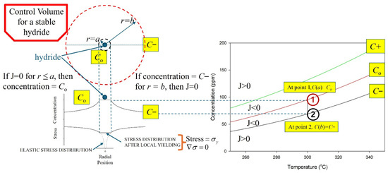
Figure 5. A representation of the cross section of the control volume of a hydride. The hydride is at the centre of the concentric circles, where r = 0. A stable hydride is when the concentration of hydrogen in a solution equals the solvus value for r ≤ a, and C− at r = b so that J = 0. The vertical line at 300 °C, connecting Co and C− in the plots on the right, indicates a stable hydride control volume. Point 1 represents a concentration state where C(a) > C₀, resulting in a negative flux (J < 0) and net hydrogen transport toward the hydride (growth). Point 2 represents a concentration state where C(b) < C−, also producing J < 0 and inward hydrogen flux toward the hydride.

The zero-flux concentrations that define the stable hydride control volume are calculated from the chemical potential with the pressure and temperature terms of the Gibbs’ energy included. The chemical potential, μ, of hydrogen atoms in the solution in the Zr lattice in the ‘ideal’ limit of dilute concentration, C, in parts-per-million by mass (wt·ppm), is as follows:

$$\mu ={\mu }^0+RT\ln C+\sigma V-ST$$

(6)

where μ⁰ is the arbitrary reference potential, R = 8.314 J/Kmol and T is the temperature in Kelvin. The last term results in the Soret effect, due to a temperature gradient; it is included for completeness but ignored for this discussion because the experiments are performed at a constant temperature. The chemical potential expressed in Equation (6) is for hydrogen in a solution in the ‘lattice’, defined by the α-Zr phase; this potential does not include hydrogen in hydride forms, nor hydrogen associated with dislocations or grain boundaries. The third term in Equation (6) is the work performed to expand the metal lattice by a mole of hydrogen atoms and is given by the product of the hydrostatic stress, σ, from the lattice expansion, and the partial molar volume, V, of hydrogen in a solution. Hydrogen moves in the solution, reaching a terminal velocity that is proportional to a conservative force given by the negative gradient of the chemical potential. The proportionality constant is the mobility, Γ, that is related to diffusivity, D, by the equation according to Einstein, D = ΓRT [11]. The flux of hydrogen in the solution, J, is the concentration times the terminal velocity, so that for a constant temperature [1],

$$\mathrm{J}=-D(\nabla C+{\displaystyle \frac{CV}{RT}}\nabla \sigma )$$

(7)

The hydrogen flux is the superposition of two independent currents: a diffusion current that depends on concentration gradients as in Fick’s Law (i.e., the first term in Equation (7)), and a drift current that depends on stress gradients (i.e., the second term in Equation (7)).

The positive sign of the partial molar volume of hydrogen in the solution indicates that hydrogen atoms expand the metal lattice locally. Hydrogen atoms will move in accordance with the drift current to regions where the lattice is expanded. The lattice is expanded by a tensile force that lowers the hydrostatic stress, thus reducing the chemical potential at the point of tension; this expansion produces a positive stress gradient that results in a negative flux by Equation (7). Positive stress gradients can be found surrounding imperfections in the metal lattice, such as dislocations, grain boundaries, and external flaws under tensile load. Positive stress gradients can also be found surrounding interstitial hydrogen atoms, so hydrogen atoms tend to gather into clusters that become more apparent at lower temperatures. The concentration of hydrogen in the solution in these gatherings eventually reaches values where metal hydrides can precipitate. Metal hydrides have bigger volumes than the metal from which they formed, so their precipitation adds further tensile stress to the surrounding metal lattice and hydrogen in the solution from farther away moves to relieve the strain. If the concentration of hydrogen in the solution drawn from farther away is sufficient to relieve the strain, then the hydride is stable: if not, then the hydride dissolves. A stable hydride is distinguished by no net movement of hydrogen in the solution, i.e., J = 0, but this is not a dynamic equilibrium: it is steady state. These conditions can be described numerically by considering the zero-flux solutions to Equation (7).

The zero-flux solution when there are no gradients in concentration or stress defines the equilibrium solvus, Co, also known as C_TSS, i.e., the region of dynamic equilibrium between hydrogen in a solution and hydrogen as hydride. By analogy with fracture mechanics, it is the region adjacent to the hydride where the stress is truncated at the combined yield strength of the hydride and metal lattice; this approach avoids the singularity of the elastic stress that would otherwise occur as the distance from the tip of the hydride approaches zero, because the stress increases with some inverse radial dependence.

There are two additional zero-flux solutions to Equation (7) that can be used to distinguish regions of concentrations and temperatures that correspond to hydride growth and hydride dissolution (i.e., J < 0 and J > 0, respectively). These zero-flux solutions can be found by equating the bracketed terms in Equation (7) to zero, rearranging terms and integrating. One of the concentration limits will be the solvus, Co, when hydrides are present. These two additional zero-flux conditions are determined by solving these two first-order equations:

$$\begin{array}{c}\hspace{1em}\hspace{1em}\hspace{1em}\hspace{1em}\hspace{1em}\hspace{1em}\hspace{1em}\hspace{1em}\hspace{1em}\hspace{1em}{\int }_{C_{-}}^{C_0}({\displaystyle \frac{\nabla \mathrm{C}}{\mathrm{C}}})=-{\displaystyle \frac{\mathrm{V}}{\mathrm{R}\mathrm{T}}}{\int }_{\sigma \left(b\right)}^{\sigma \left(a\right)}\nabla \sigma \hfill \\ \mathrm{and}\hfill \\ \hspace{1em}\hspace{1em}\hspace{1em}\hspace{1em}\hspace{1em}\hspace{1em}\hspace{1em}\hspace{1em}\hspace{1em}\hspace{1em}{\int }_{C_0}^{C_{+}}({\displaystyle \frac{\nabla \mathrm{C}}{\mathrm{C}}})=-{\displaystyle \frac{\mathrm{V}}{\mathrm{R}\mathrm{T}}}{\int }_{\sigma \left(b\right)}^{\sigma \left(a\right)}\nabla \sigma \hfill \end{array}$$

(8)

Cylindrical coordinates shown in the upper left corner of Figure 5 are consistent with the geometry of the hydrides formed in the bulk; these concentric circles define the control volume of a hydride. A hydride is idealized as a circle in the figure. Hydrides first form as long needles of γ-phase [12]. In the figure, the hydride extends into the plane of the diagram. The integration limits a and b in Equation (8) are relative to the hydride: a is the distance from the tip of the hydride, defining a region where the stress is truncated at the combined yield strength of the hydride and metal lattice, and b is where the stress has decreased from the value at distance a (i.e., the combined yield strength) to the background value where the stress gradient vanishes. b defines the extent of the control volume associated with a stable hydride. For a hydride to be stable J = 0, there is no net flux of hydrogen in the solution. For a stable hydride, the concentration of hydrogen in the solution will be at the solvus, Co, in the small region adjacent to the hydride surface, i.e., at r ≤ a, and at C− at the periphery of the control volume, i.e., at r = b, so that J = 0.

The difference in hydrostatic stress at these integration limits is assumed to be proportional to the yield strength, σ_y, (i.e., σ(a) − σ(b) = −Kσ_y), where the difference is relative to the reference value in the metal lattice that is set to zero. The proportionality constant, K, will be interpreted as an elastic stress concentration factor that provides a measure of the sink strength of the hydrostatic stress field for hydrogen. Values of K will be geometry-dependent and different for hydrides forming at dislocations, or in the bulk, or at a crack tip. For a stress riser under plane stress, for example, a ‘thin’ hydride in the lattice, K could be about two [1]. For a ‘broad’ crack under plane strain, K is 2.4, calculated from one-third of the trace of the stress tensor (see Section 5.3.1 of [13] and Equation 2.85 in [14] for an infinitely sharp Mode 1 plane-strain perfectly plastic crack tip). The parameter K is a dimensionless number: it is not a stress intensity factor; it is an elastic stress concentration factor.

The two zero-flux solutions, in addition to the solvus solution for Co given by Equation (5), are as follows [1]

$$C_{-}(T)=C_{\mathrm{o}}(T)\exp \left({\displaystyle \frac{-KV{\sigma }_y}{RT}}\right),$$

(9)

$$C_{+}(T)=C_{\mathrm{o}}(T)\exp \left({\displaystyle \frac{+KV{\sigma }_y}{RT}}\right).$$

(10)

These concentrations, C− and C+, will constrain the magnitudes of the concentrations in the solution that can occur in the presence of hydrides when J = 0. The concentrations C− and C+ have been identified in X-ray diffraction studies [15], as shown in Figure 6.

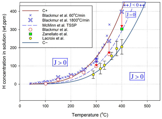
Figure 6. The three curves show the three J = 0 solutions to the flux equation, Equation (7), with Co approximated by TSSP and C+ and C− calculated with Equations (9) and (10). The data are described in (15).

Inside the metal, the hydrogen in the solution and hydrogen in hydrides are confined by the hydrostatic pressure (i.e., stress) of the metal. When a hydride forms, it pushes the lattice apart, producing a tensile stress gradient. Hydrogen moves to relieve the resulting strain. A stable hydride can be defined by a control volume surrounding the hydride. In the small volume adjacent to the hydride, the concentration of hydrogen in the solution is at the solvus value, Co, and the concentration and stress gradients are zero. Where the stress gradient again goes to zero defines the extent of the control volume that is proposed to stabilize hydrides. The concentration of hydrogen in the solution at the extent, C−, is such that the net flux of hydrogen in the solution towards and away from the hydride is zero; hence, the hydride is stable. The clouds and atmospheres of hydrogen in the solution surrounding the hydrides ‘cloaks’ the hydrides when they are stable.

At the extent of stable hydride control volumes, and between control volumes, the gradients of concentration and hydrostatic stress are equal to zero. The inference is that stable hydrides and hydrogen in the solution between stable hydride control volumes both experience the same hydrostatic stress. Thus, between stable hydrides, there is no change in internal hydrostatic stress (pressure) when hydrides precipitate or dissolve, as represented in Figure 7.

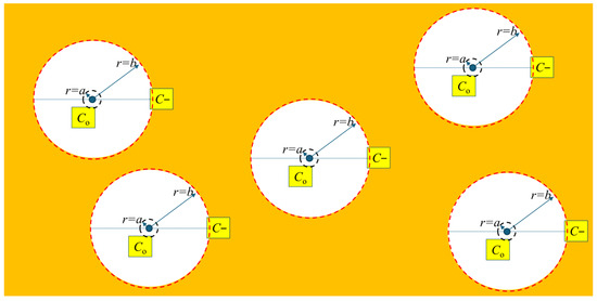
Figure 7. In the shaded region between stable hydrides, the concentration of hydrogen in the solution is C− and the hydrostatic stress is constant (not to scale).

5. Athermal Hydrides Determined from X-Ray Diffraction

Diffraction of X-rays is a direct method to observe hydrides precipitating and dissolving by following measured areas of hydride diffraction peaks to temperatures where signals are first observed or completely disappear, respectively. The X-ray results showed evidence that athermal hydrides–hydrides form without concomitant exothermic heat being released; hence, these hydrides were called athermal. Athermal hydrides are not detected with DSC.

A schematic diagram of the X-ray diffraction experiment performed at the Argonne Advanced Photon Source is shown in Figure 8, adapted from [1], where the details of the experiment can be found.

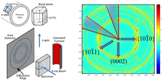
Figure 8. A schematic diagram of the X-ray diffraction experiment [1].

Athermal hydrides are associated with dislocations that have ready-made Cottrell atmospheres of surrounding hydrogen in the solution that can condense without releasing heat when hydrides form during cooling. At temperatures where stable hydrides do not exist, the concentration of hydrogen in the solution is not uniform; hydrogen tends to cluster and to gather more around dislocations that are surrounded by tensile stress gradients. Hydrogen ‘captured’ in these stress fields does not have the kinetic energy that free hydrogen atoms have in the bulk: the movement of the captured hydrogen is constrained by the stress field; heat is given off by the hydrogen that is captured; and this exothermic process is independent of hydrides forming. When the temperature is lowered, eventually, stable hydrides form at these dislocation sites. In this instance, there is no need to draw hydrogen from the bulk; the hydrogen that stabilizes the hydride is already available in the atmosphere of hydrogen in the solution surrounding the dislocation. Because the hydrogen captured in the atmosphere of the dislocation has lower kinetic energy than free hydrogen, there is no measurable heat released when the atmosphere of the dislocation transforms to become the stabilizing hydrogen atmosphere of the hydride. Thus, stable athermal hydrides form first on cooling at dislocation sites.

Figure 9a shows a DSC heat flow curve for cooling. There is no dramatic change in heat flow until about 280 °C, other than the slightly sloping ‘background’. Figure 9b shows the areas of hydride X-ray diffraction lines with cooling. Hydrides are observed to form at 315 °C and the areas of the diffraction lines increase as the temperature is lowered until about 260 °C. Hydrides are forming at temperatures where there are no DSC thermal signals. These hydrides are gamma athermal hydrides, labelled γ^a.

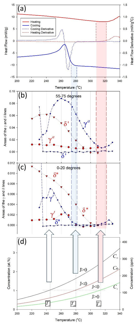
Figure 9. (a) DSC heat flow curves and (b,c) areas of hydride diffraction peaks, obtained during cooling and heating within two angular regions around the diffraction ring [1]. The bottom plot (d) shows how the concentrations of hydrogen in the solution changes with temperature according to the control volume interpretation. Hydride diffraction peaks are seen to start cooling at 315 °C in (b) but no thermal signal is seen until ≈280 °C with DSC in (a). This difference is attributed to athermal hydrides that do not give a measurable DSC signal when they precipitate.

At temperatures below where stable athermal hydrides first form on cooling at dislocations, thermal hydrides can form in the bulk. Thermal hydride precipitation happens when the solvus, i.e., TSS, conditions are met. These hydrides have thermal signals because there are no pre-existing atmospheres of hydrogen in the solution that are locally available, so hydrogen must be drawn from the free hydrogen in the bulk and captured within the stress field of the control volume surrounding the hydride, and the capturing process releases heat—in this instance, this exothermic process is directly dependent on hydrides forming and is why DSC records exothermic differential heat flow when the solvus is reached. The third plot in Figure 9 shows thermal hydrides, labelled γ^t, first precipitating at about 280 °C, coinciding with the temperature, where a large change in DSC heat flow is observed in the first plot. The temperature where this large change begins is called the onset temperature and is associated with the solvus.

It is proposed that when cooling from temperatures where no stable hydrides are present, unstable hydrides form, then dissolve, then form and then dissolve, oscillating back and forth, because the stability conditions cannot be met (i.e., hydrides are stable when surrounded by a cloud or atmosphere of hydrogen in a solution such that J = 0). As the temperature is lowered, oscillating hydrides eventually stop oscillating when the solvus conditions are reached and stable hydrides form.

Stable thermal hydrides dissolve with heating, persisting to about 315 °C, which is T+ associated with C− in the figures. The apparent temperature hysteresis seen with DSC is the difference between the temperatures where athermal hydrides form and thermal hydrides form and dissolve. In the example shown in Figure 9, the temperature hysteresis would be 315 °C − 280 °C = 35 °C.

6. The Phase Rule and Hysteresis

The control volume explicitly includes two concentrations that are associated with J = 0. The first concentration is Co, which is associated with the solvus; this is the no gradients in stress or concentration solution. The second concentration is C−. This concentration is associated with the control volume of a stable hydride; it is found at the extent of the control volume and is also associated with no flux when the terms with gradients in stress and concentration cancel. These concentrations are linked by the vertical line between C− and Co at 300 °C in Figure 5. For example, Co is the concentration for r ≤ a, and C− at r = b in the stable hydride control volume. The two concentrations are allowed by Gibbs’ phase rule, Equation (2), for the stable hydride because there are two stress states. For r ≤ a, the stress is truncated at the yield strength. For r = b, the stress equals the hydrostatic stress in the unstressed bulk.

The assumption for the reduced ‘condensed’ phase rule is that there is only one pressure (i.e., stress in a solid) and it does not change, so there is no degree of freedom associated with stress (i.e., Vdp = 0). In the control volume, there are two fixed-point stresses at different locations, and two dependent concentrations at the same temperature. Thus, it appears that the condensed phase rule, Equation (3), applies in the region between control volumes, which is the shaded region in Figure 6. Gibbs’ phase rule, Equation (2), applies to the stable hydride where there are two independent stress states and hence, another degree of freedom.

There are three concentrations for each temperature in Figure 5, suggesting that an additional degree of freedom might be included in Gibbs’ phase rule. For example, the vertical line at 300 °C could be extended to include C+, which would add another degree of freedom if C+ were independent. But, the three concentrations, C−, Co, and C+, are not independent. From Equations (9) and (10):

$$C+=C{\mathrm{o}}^2/C-$$

(11)

Thus, C+ does not add an additional degree of freedom and Gibbs’ phase rule needs no modification.

7. The Cycle-Pause Experiment

This experiment highlights the time required to form a stable hydride control volume in Zr-2.5Nb after heating and cooling to a fixed temperature. Experimental data are from the long-duration DSC cyclic experiments presented in [16]. Times at an isothermal test temperature of 300 °C were varied up to 60,000 min for two conditions: one where the test temperature was arrived at by cooling from 390 °C, and another where the test temperature was obtained after heating from 150 °C. At various times, the isothermal temperatures were interrupted when the specimen under test was cooled to 150 °C in the DSC and exothermic onset precipitation temperatures were measured. After each onset precipitation temperature measurement, the specimen was either heated to the test temperature, 300 °C, where it was held for a longer time in a series of experiments called ‘heat and hold’, or heated to 390 °C and then cooled to the test temperature, where it remained for a longer time in a separate series of experiments called ‘cool and hold’. The hold times were not randomized.

The results of the interrupted isothermal experiments are presented in Figure 10 and Figure 11. Concentrations were not provided in the original study, just DSC temperatures. Starting with the DSC heat flow curves in Figure 2c,d in [16], the endothermic maximum slope temperature was 369.8 °C and the peak endothermic temperature, which is equivalent to C− [7], was lower by about 17 °C. The onset temperature was 325.5 °C. Figure 10 was constructed to conform to these values, as shown by the dash-dot grey lines. In addition, the C− curve had to conform to the previously measured concentrations (hot vacuum extraction mass spectroscopy) and the corresponding DSC endothermic ‘peak’ temperatures, shown by the black circular markers for Zr-2.5Nb with a fully decomposed beta-phase [17] (i.e., %Nb in the beta-phase was equal to 94% in accordance with the prior 100 h anneal at 500 °C for this material [16]). Thus, the C+, Co, and C− curves were determined. The estimated total concentration in the specimen was 122 wt·ppm. The horizontal grey dash-dot line at 122 wt·ppm is horizontal, in accordance with the assumption, for the sake of discussion, that there are no athermal hydrides present. Prior to testing, the specimen was heated at 500 °C for 100 h, which arguably decreased the dislocation density and the numbers of athermal hydrides on cooling—thus, for this discussion, the solvus onset temperatures were associated with the total hydrogen in the specimen. Absolute concentrations are not needed to illustrate the time evolution.

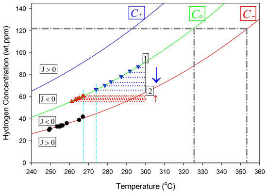
Figure 10. A series of ‘cyclic’ experiments used to monitor C(b) in Zr-2.5Nb as a function of time for specimens that were cooled or heated to the isothermal temperature, 300 °C, where they were held for times up to 60,000 min and then cooled and onset-precipitation temperatures were recorded: blue down-pointing triangles for specimens were initially cooled, and red up-pointing triangles for specimens were initially heated to the isothermal temperature. The arrows show the time sequence of the measurements. The black circular markers from [17] show the DSC endothermic ‘peak’ temperatures for the measured total hydrogen concentrations in Zr-2.5Nb. Point 1 corresponds to the concentration state reached after cooling to 300 °C (C(b) → C₀), and Point 2 to that reached after heating (C(b) → C−), illustrating solubility hysteresis at the isothermal temperature.

Figure 11. Time dependence for the changing C(b) concentrations in Figure 10.

When cooling from temperatures where there are no stable hydrides, the concentration of hydrogen in the solution is initially the same everywhere on average if the specimens are small and the cooling rate are slow enough so that there is no thermal temperature gradient through the specimen. There are no control volumes, and there are no C(a) and no C(b) if hydrides have not formed. Precipitates that form in specimens cooled to the test temperature of 300 °C will have C(a) equal to the solvus value, Co, in the small region adjacent to the hydride, Point 1 in Figure 10. The concentration of hydrogen in the solution just outside this adjacent region will be slightly less because of the hydrogen lost to form the hydride. The conditions are such that J < 0, and hydrogen moves from the bulk into the control volume of the hydride to relieve the strain caused by the formation of the hydride: to fill the void, as it were. Thus, the concentration of hydrogen in the solution in the bulk, C(b), reduces with time as the hydrogen in the solution moves into the control volume. Eventually, C(b) reaches C−, where J = 0 and no more hydrogen moves, so the hydride is stable; this is Point 2. Thus, there is a lag in the time to reach C(b) compared with the time to reach C(a): C(a) is reached almost immediately, while it takes more time for the concentration in the much larger region between control volumes to reach C(b), relatively speaking.

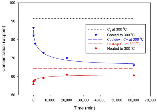
Interrupting this fall of C(b) to C− periodically to measure the temperature where the hydrogen in the solution in the bulk at the test temperature precipitates allows the temporal descent of C(b) to be observed. The descent is empirically found to vary roughly as an exponential function that depends on the square root of time falling about halfway after 15 ± 8 h, based mostly on three data: see Figure 11. In an X-ray diffraction study of Zircaloy reported by Lacroix et al., the descent was complete after 2 h at 380 °C, see Figure 5 in [18]. At a lower temperature, the descent is expected to take longer because of slower diffusion, but comparisons of these descent times can only be superficial because these alloys (Zr-2.5Nb and Zircaloy) and their prior heat treatments were different; still, time scales of hours seem to be appropriate.

For specimens heated to the test temperature, the bulk concentrations of hydrogen in the solution rise with time to C− at Point 2 in Figure 10. The rise with time is shown in Figure 11, where the curve through the data is an empirical saturating exponential with a square root of time argument. The concentrations approach halfway to their final value after roughly 17 h, but it appears that within the error of measurements of a few degrees Celsius in the DSC determinations of the onset, it is also reasonable to say that the final concentration was reached within the first 10 min at the test temperature when heated at 10 °C/min to the test temperature. Any rise and fall times inferred from Figure 11 are very rough.

For specimens heated to the test temperature, the concentrations of hydrogen in the solution in the small region adjacent to the hydride, C(a), will reach the solvus value immediately compared with the concentration at the periphery of the control volume, C(b), which will take longer because of the much larger volume of the bulk between control volumes. Thus, C(b) lags C(a). For specimens heated to the test temperature, hydrogen in the solution in the bulk slowly rises as hydrides formed at temperatures below C− for 300 °C dissolve, shown approximately by the left vertical dashed line in Figure 10.

The conventional interpretation cannot explain the declining concentrations for the cool-and-hold results shown in Figure 10 and Figure 11. A version of the conventional interpretation has been implemented into the nuclear fuel performance code BISON being developed at Idaho National Laboratory to model the concentration of hydrogen in a solid solution and in hydrides [19]. TSSP is modelled as an unstable super-solubility state that decays to TSSD, or some close version of TSSD that would be the ‘true’ solvus at 300 °C. But, if TSSP were metastable, then the TSSP curve would decline with time, as would the onset curve, which is the basis for the measurement of the decline at 300 °C. It would be impossible to monitor the time of the descent of the concentration at 300 °C by intermittently cooling to find the onset temperature, because the declining concentrations of the onset and TSSP curves would always be below the declining concentrations at 300 °C. Cooling could never lead to more precipitation because the TSSP curve would never be crossed if it too were declining like the concentration at 300 °C. Figure 10 shows how the declining concentration at 300 °C is transformed by a ‘time-stable’ onset curve to the observed declining measured onset temperatures over time (i.e., the temperatures associated with the blue triangles that decorate the onset curve in Figure 10). This conventional ‘non-explanation’ of the declining onset temperatures with time following isothermal holds should provide a strong counterargument against the claim that TSSP is metastable. In the words of the current interpretation, the solubility limit, defined by the onset temperature, does not vary with time, which is expected for a parameter that is only defined at equilibrium. Finally, the onset temperature measurements rise with time for the heat-and-hold experiments. This rise could not happen if the precipitation onset temperatures were declining.

The idea of two solvi is discredited by the results of Figure 10, which show that the specimen evolves to the same final state, regardless of whether the specimen was heated or cooled to the test temperature of 300 °C, i.e., the same control volume represented by Points 1 and 2 in Figure 10 is reached after C(b) reaches C- from above or below. Figure 11 shows that the rise and fall of C(b) to Point 2 happens at the same rate. The rates must be the same for the final state at 300 °C to be stable with respect to thermal fluctuations. The results of Figure 10 and Figure 11 provide experimental evidence that there is no hysteresis.

8. The TSSP–TSSD Paradox

The current interpretation resolves the TSSP–TSSD paradox. If hydrides are present after heating and cooling to the same temperature, then the concentrations of hydrogen in the solution will be at the TSSD and TSSP values, respectively, according to the conventional interpretation. The paradox occurs when samples that are heated and cooled to the same temperature are connected, so hydrogen can flow between the samples. What will be the concentration of hydrogen in the solution in the connected samples at equilibrium? Will the different TSSP and TSSD concentrations of hydrogen in the solution be maintained or will hydrogen flow from the sample cooled to the common temperature to the sample heated to the common temperature because the TSSP concentration is higher than the TSSD concentration? If hydrogen flows from the cooled to the heated sample, then will all hydrides not end up in the heated sample and the final concentration of hydrogen in the solution will be the TSSD value? It would be strange indeed to see hydrides at constant temperatures in both samples initially and then hydrides only in the heated sample after time—this result seems to violate the Second Law. The current interpretation resolves this strange implication of the conventional interpretation. There is not a single concentration of hydrogen in the solution when hydrides are present. Instead, there are many concentrations within a gradient, starting with the concentration of hydrogen in the solution at the solvus in the region adjacent to the hydride and ending with the concentration being at C− at the extent of the control volume of a stable hydride. The control volume structure is the same, regardless of whether the common temperature was reached by heating or cooling; thus, there is no hysteresis.

9. Apparent Hysteresis

The apparent hysteresis can be explained with a straightforward extension of the explanation of the results shown in Figure 10. The explanation for the apparent hysteresis follows the time evolution of C(b), i.e., the concentration at r = b, and in the bulk between hydrides. When cooling from a temperature where there are no stable hydrides, hydrides will eventually form. Surrounding the hydride will be a small volume where the hydrogen in the solution has a concentration, C(a), that is close to the solvus, Co. Outside of this small volume, hydrogen in the solution in the bulk, C(b), moves to relieve the strain that happens when the hydride forms. Given a few hours, C(b) reduces to C− and a stable hydride is formed, i.e., J = 0: this is the explanation that went with Figure 10 and Figure 11. But instead, if the cooling continues at, for example, 10 °C/min, then C(b) does not appreciably drop to C− in the time of the DSC measurement over a small temperature range of a few degrees. The result is that C(b) follows Co, with cooling of 10 °C/min. More precisely, on cooling with hydrides present, the bulk concentration is limited by C+ until the extent of the hydride stability range at C- before dropping to Co, as shown in Figure 6 and described in the discussion of Figure 8 in [1] where Co is labelled C_TSS. But the time before the drop to Co is so short compared with the subsequent drop to C− that for discussion, it is assumed that the bulk follows Co with standard experimental cooling rates.

When hydrides are dissolving during heating, C(a) follows Co, like before. In the bulk, C(b) lags C(a) because of its larger relative volume, but it is now following C− if hydrides are dissolving.

Thus, the concentration of hydrogen in the solution in the bulk, C(b), follows Co during precipitation and C− during dissolution; this presents as a hysteresis.

If the turn-around time from cooling to heating is ‘fast’, then at the lowest temperature of cooling, there will be no time for C(b) to fall to C−. When heating starts, there will be a pause before hydrides dissolve, because initially, C(b) will be in the region where J < 0, i.e., within the space between the three curves, see Figure 5. As the temperature increases, the concentration in the solution at the end of cooling will stay at that value until the concentration intersects with the C− curve at a higher temperature, i.e., the concentration will move horizontally with the temperature across the C-T plot to C−. Beyond the temperature of C−, there is a positive flux of hydrogen away from the hydrides, i.e., J > 0, and hydrides dissolve. If the turn-around time takes hours, then C(b) at the lowest cooling temperature will have time to fall to C−. In this case, there will be no pause before hydrides dissolve with heating.

Thus, apparent hysteresis depends on the relative rate of C(b) descending to C− compared with the rate the temperature is scanned in measurements like DSC. For slow scans (hours) like those in Figure 10, there is no hysteresis: the same final control volume is reached regardless of whether the test temperature was reached by heating or cooling. If the rate of temperature scans is fast (minutes), then there is an apparent hysteresis that is a consequence of the lag of C(b) relative to C(a) to reach the conditions for a stable hydride control volume, and the lag is a consequence of different volumes: the volume of the bulk between stable hydrides is much bigger than the volume surrounding the hydride, for r ≤ a, within the control volume.

10. Discussion

The Gibbs’ phase rule given by Equation (2) is applicable for the H-Zr system, i.e., F = C + 2 − P. For a two-component, two-phase system, the degrees of freedom are two. If we choose temperature as one independent variable, then concentration can be one dependent variable: in this case, we choose the no-gradients solution of Equation (7) that is associated with dynamic equilibrium, J = 0, and the solvus. The second independent variable chosen is hydrostatic stress. In this case, C− is the corresponding dependent variable that is associated with J = 0 and the concentration of hydrogen in the solution at the periphery of the control volume of a stable hydride.

The control volume structure follows from Gibbs’ phase rule. The J = 0 condition is fundamental because this leads to two dependent concentrations: Co and C−. These two concentrations cannot simultaneously and separately exist in equivalent regions in contact with each other in the same material, because the hydrogen in the solution would flow in reaction to the concentration difference until there was no difference. But, these two concentrations can exist simultaneously if one, Co, is contained within a region inside a second region where the concentration at the extent is C−, and between these regions there is a yield stress gradient that makes the material different at either end of the gradient. Such is the control volume of a stable hydride shown in Figure 5. Amazingly, the control volume is a direct consequence of Gibbs’ phase rule.

A similar argument has been made to understand how gamma and delta hydrides can be observed simultaneously with hydrogen in the solution. Hydrogen in the solution cannot be in equilibrium with both gamma and delta at the same time. Some have argued that equilibrium does not apply because gamma hydride is metastable. But gamma and delta can be observed simultaneously if the delta is surrounded by a layer of gamma [1,20], Figure 12. In this case, the gamma is in equilibrium with the hydrogen in the solution, and the delta is in equilibrium with gamma, but the delta never sees the hydrogen in the solution. Thus, the phase rule was instrumental in ascertaining the structure of the hydride phase.

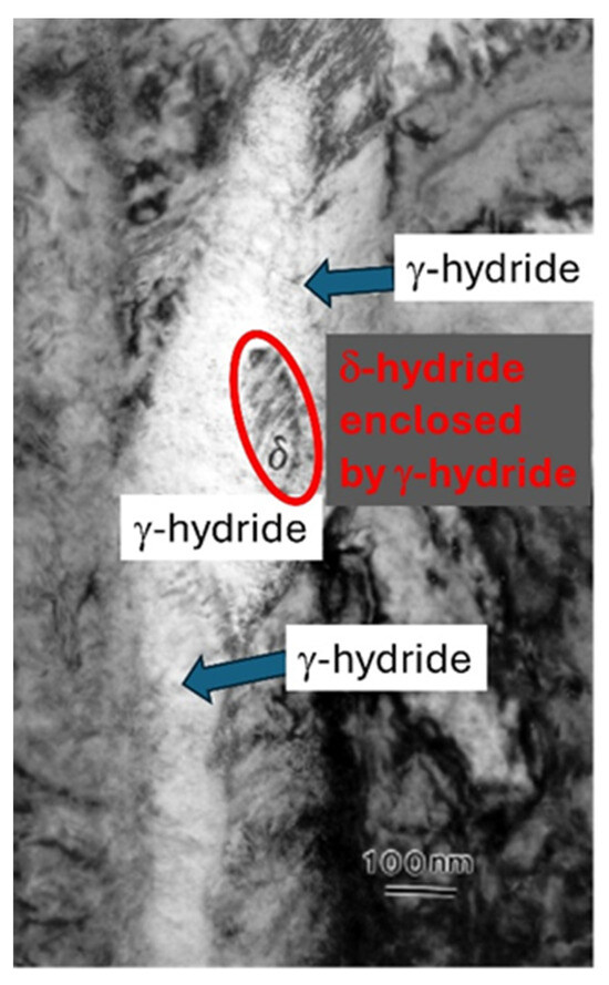
Figure 12. TEM micrograph showing δ-hydride surrounded by γ-hydride in Zr-2.5Nb [1], in accordance with the phase diagram (Figure 4), based on [20].

The association of a surrounding cloud or atmosphere of hydrogen in the solution that stabilizes a hydride when it forms can be inferred from equations of force and equations of Gibbs’ free energy. In the current study, the forces moving hydrogen in zirconium alloys were determined from the negative gradient of the chemical potential that was written as a flux of hydrogen in solid solution. Special cases were identified when the forces and flux were zero, which were used to construct a control volume description of a stable hydride. The control volume description is also consistent with previous Gibbs’ free energy arguments. Density functional theory (DFT) calculations showed “that precipitation of hydrides is not thermodynamically favourable for Zr-H solid solutions containing less than 300 wt·ppm H”, yet hydrides are clearly seen, “suggesting that a mechanism must cause local concentration of H atoms to a greater amount than found globally in experimental samples containing hydrides” [21]. The influx of hydrogen in the solution into the control volume to form a stable hydride is the concentrating mechanism required to overcome the positive free energy calculated with DFT for hydride precipitation when the total concentrations are below 300 wt·ppm [1,21]. Thus, the control volume description is consistent with the interpretations of the special cases of zero forces and hydrogen flux and free energy DFT expectations.

The control volume provides an interesting view of the phase field method that is used to make sharp interfaces more diffuse in mathematical computer simulations. An example of a possible sharp interface is between a hydride and the surrounding metal. Sharp interfaces are difficult to represent mathematically because derivatives become infinite, so an order parameter, ϕ, is introduced that is varied to make the interface change continuously. For two-phase materials, ϕ is typically fixed at zero and one for the individual phases, and the interface is the domain where 0 < ϕ < 1. For the phase field formalism, Gibbs’ energy is written in terms of three intensive variables: the order parameter, the concentration, and the temperature; G(ϕ, C, T) [22].

Compare this formalism with the control-volume interpretation for which the three intensive Gibbs’ variables are yield stress, concentration, and temperature: G(σ, C, T). Recall for two components and two phases, Gibbs’ phase rule (Equation (2)) says that there are two independent intensive variables: we chose temperature and yield stress; concentration is then the dependent variable that results in Co and C−, respectively, for J = 0, as previously discussed.

The phase field formalism has adopted the order parameter instead of the gradient of the yield stress. It is suggested that the process of varying the order parameter to find solutions that agree more-or-less with observations will converge on a solution that is essentially C−. Thus, the phase field method may be eclipsed, in part, by the control-volume formalism.

Finally, there is no spatial scale dependence in the flux equation, Equation (7), which means that the implications of the zero-flux solutions and the control volume representation should likewise be scale independent and be valid for the very small and the very large. In the current analysis, free hydrogen in solid solution preferentially gathers and then condenses as hydride particles on high energy sites (i.e., dislocations), where the local symmetry associated with the underlying hexagonally close packed crystal structure is broken. The result is that hydrides form on a variety of different broken symmetry planes that emerge following cooling after prior heat treatment. Hydrides tend to form preferentially on low-energy habit planes. Hydrogen in the solution that does not become a hydride contributes to the hydrogen in the solution in the control volumes that stabilize the hydrides that form.

11. Practical Application: Temperature Maneuvers

Figure 13 shows a temperature maneuver that can form a stable hydride [23]. In this example, a zirconium alloy containing hydrogen is cooled to 270 °C, Point 3, and then heated to 300 °C. A stable hydride will form at 300 °C if the concentration of hydrogen in the solution at Point 3, i.e., C(b), does not have time to move towards C− before being heated to 300 °C. In this case, the concentration of hydrogen in the solution follows the horizontal line to Point 2 during heating to 300 °C. Following this maneuver, stable hydrides are created in the bulk at 300 °C, as indicated by the vertical line between Points 1 and 2. If instead of the maneuver, cooling was just to 300 °C, then it could take much longer to form a stable hydride, because of the time it takes for C(b) to drop to C−, as shown in Figure 10 and Figure 11.

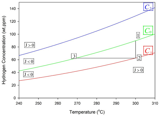
Figure 13. If cooling starts from temperatures where stable hydrides do not exist to Point 3 at 270 °C and then heating raises the temperature to 300 °C, the result will be a stable hydride at 300 °C. Point 1 corresponds to the solvus concentration (C₀) at the hydride interface, and Point 2 to the outer boundary concentration (C−), giving zero net hydrogen flux.

12. Conclusions

The precipitation–dissolution hysteresis of hydrides during thermal cycling has been found to depend on athermal hydrides and time to form a stable hydride control volume. The temperature hysteresis is the difference between the temperatures where athermal hydrides and thermal hydrides form.

Experimental data were constructed that show there is no hydride precipitation–dissolution hysteresis. The same final state was found to be independent of whether the isothermal test temperature was arrived at by heating or cooling. This result resolves the TSSD–TSSP paradox. The apparent hysteresis seen in measurements such as DSC disappears with time.

Gibbs’ phase rule has been used in a binary two-component two-phase system to construct the structure of the stable hydride phase in the H-Zr system. The number of independent degrees of freedom is two. The independent variables for Gibbs’ energy, G(σ, C, T), were chosen to be yield stress and temperature. The dependent variables were the solvus, Co, for T, and C− for the yield stress: the solvus depends only on temperature and C− depends on yield strength and the solvus. The constraint that both concentrations exist simultaneously when there is no net flux of hydrogen in the solid solution led to the control volume depiction of a stable hydride with the solvus concentration in the small volume adjacent to the hydride and C− at the extent of the control volume, so that J = 0. Between these concentrations is a region where a stress gradient exists that stabilizes the concentrations.

The reduced ‘condensed’ phase rule applies when the stable hydride control volume is the phase; in this case, the internal stress between the control volumes of stable hydrides is constant and the degrees of freedom are reduced by one.

The classic measurements called TSSD and TSSP do not follow Gibbs’ phase rule because the concentrations do not appear at the same time.

The implications for phase field methods were discussed. This method to make phase boundaries more diffuse might not be needed if instead the control-volume interpretation is adopted.

The control volume description derived from zero-flux (zero force) conditions for hydrogen in the solution is also consistent with previous Gibbs’ free energy calculations, based on density functional theory, that predict that the precipitation of hydrides is not thermodynamically favourable unless there is a mechanism to concentrate hydrogen in the solution around hydrides to overcome the positive free energy that otherwise occurs. Thus, the control volume description is consistent with independent interpretations based on forces or energies.

References

- McRae, G.A.; Coleman, C.E. Precipitates in metals that dissolve on cooling and form on heating: An example with hydrogen in alpha-zirconium. J. Nucl. Mater. 2018, 499, 622–640. [Google Scholar] [CrossRef]
- Erickson, W.H.; Hardie, D. The influence of alloying elements of the Terminal Solubility of Hydrogen in Zirconium. J. Nucl. Mater. 1964, 13, 254–263. [Google Scholar] [CrossRef]
- Gibbs, J.W. On the Equilibrium of Heterogeneous Substances. Transactions of the Connecticut Academy, III; pp. 108–248, October 1875–May 1876; pp. 343–524, May 1877–July 1878.
- CSA N285.8:21; Technical Requirements for In-Service Evaluation of Zirconium Alloy Pressure Tubes in CANDU Reactors. Canadian Standards Association: Mississauga, ON, Canada, 2021.
- Puls, M.P. The Effects of Hydrogen and Hydrides on the Integrity of Zirconium Alloy Components—Delayed Hydride Cracking; Engineering Materials; Springer: London, UK, 2012. [Google Scholar]
- Köonigsberger, E.; Eriksson, G.; Oates, W.A. Optimisation of the thermodynamic properties of the Ti-H and Zr-H systems. J. Alloys Compd. 2000, 288, 148–152. [Google Scholar] [CrossRef]
- McRae, G.A.; Coleman, C.E. Thermodynamics and Kinetics of Delayed Hydride Cracking in Zirconium Alloys: A review. J. Nucl. Mater. 2024, 601, 155006. [Google Scholar] [CrossRef]
- Cameron, D.J.; Duncan, R.G. On the Existence of a Memory Effect in Hydride Precipitation in Cold-Worked Zr-2.5% Nb. J. Nucl. Mater. 1977, 68, 340–344. [Google Scholar] [CrossRef]
- Ritchie, I.G.; Pan, Z.-L. Internal Friction and Young’s Modulus Measurements in Zr-2.5Nb Alloy Doped with Hydrogen. In M3D: Mechanics and Mechanisms of Material Damping, ASTM STP 1169; Kinra, V.K., Wolfenden, A., Eds.; American Society for Testing and Materials: West Conshohocken, PA, USA, 1992; pp. 385–395. [Google Scholar]
- Ritchie, I.G.; Sprungmann, K.W. Hydride Precipitation in Zirconium Studied by Low-Frequency Pendulum Techniques. J. Phys. 1983, 44, C9-313–C9-318. [Google Scholar] [CrossRef]
- Einstein, A. Über die von der molekularkinetischen Theorie der Wärme geforderte Bewegung von in ruhenden Flüssigkeiten suspendierten Teilchen. Ann. Phys. 1905, 322, 549–560. [Google Scholar] [CrossRef]
- Bradbrook, J.S.; Lorimer, G.W.; Ridley, N. The precipitation of zirconium hydride in zirconium and Zircaloy-2. J. Nucl. Mater. 1972, 42, 142–160. [Google Scholar] [CrossRef]
- Kanninen, M.F.; Popelar, C.H. Advanced Fracture Mechanics; Oxford University Press: Oxford, UK, 1985. [Google Scholar]
- Hellan, K. Introduction to Fracture Mechanics; McGraw-Hill Book Company: New York, NY, USA, 1985. [Google Scholar]
- McRae, G.A.; Coleman, C.E. Zirconium hydride precipitation in Zircaloy-4 during rapid cooling followed by isothermal interludes observed with synchrotron X-ray diffraction. J. Nucl. Mater. 2022, 565, 153729. [Google Scholar] [CrossRef]
- Hanlon, S.M.; Skippon, T.; Muir, I.; Bickel, G.A.; Hilton, V. The Effect of Long Isothermal Holds on Hydride Dissolution and Precipitation Behavior in Zircaloy-2 and Zr-2.5Nb. In Zirconium in the Nuclear Industry: 20th International Symposium; Yagnik, S.K., Preuss, M., Eds.; ASTM International: West Conshohocken, PA, USA, 2023; pp. 723–754. [Google Scholar] [CrossRef]
- Khatamian, D. Effect of β-Zr decomposition on the solubility limits for H in Zr-2.5Nb. J. Alloys Compd. 2003, 356, 22–26. [Google Scholar] [CrossRef]
- Lacroix, E.; Motta, A.T.; Almer, J.D. Experimental determination of zirconium hydride precipitation and dissolution in zirconium alloy. J. Nucl. Mater. 2018, 509, 162–167. [Google Scholar] [CrossRef]
- Passelaigue, F.; Lacroix, E.; Pastore, G.; Motta, A.T. Implementation and Validation of the Hydride Nucleation-Growth-Dissolution (HNGD) model in BISON. J. Nucl. Mater. 2021, 544, 152683. [Google Scholar] [CrossRef]
- Root, J.H.; Small, W.M.; Khatamian, D.; Woo, O.T. Kinetics of the d to g zirconium hydride transformation in Zr-2.5 Nb. Acta Mater. 2003, 51, 2041–2053. [Google Scholar] [CrossRef]
- Lumley, S.C.; Murphy, S.T.; Grimes, R.W.; Wenman, M.R.; Burr, P.A.; Chroneos, A.; Chard-Tuckey, P.R. The thermodynamics of hydride precipitation: The importance of entropy, enthalpy and disorder. Acta Mater. 2014, 79, 351–362. [Google Scholar] [CrossRef]
- Qin, R.S.; Bhadeshia, H.K. Phase field method. Mater. Sci. Technol. 2010, 26, 803–811. [Google Scholar] [CrossRef]
- Coleman, C.E.; Cheadle, B.A.; Ambler, J.F.R.; Lichtenberger, P.C.; Eadie, R.L. Minimizing hydride cracking in zirconium alloys. Can. Metall. Q. 1985, 24, 245–250. [Google Scholar] [CrossRef]
Disclaimer/Publisher’s Note: The statements, opinions and data contained in all publications are solely those of the individual author(s) and contributor(s) and not of MDPI and/or the editor(s). MDPI and/or the editor(s) disclaim responsibility for any injury to people or property resulting from any ideas, methods, instructions or products referred to in the content. |
© 2026 by the authors. Licensee MDPI, Basel, Switzerland. This article is an open access article distributed under the terms and conditions of the Creative Commons Attribution (CC BY) license.