Prediction of Prestress Changes in Concrete Under Freeze–Thaw Cycles Based on Transformer Model

Abstract

Given that freeze–thaw damage of prestressed concrete significantly threatens structural service life and that existing conventional simulation techniques fail to capture prestress time series, this paper proposes a deep learning prediction model based on the Transformer model. The model integrates a multi-head self-attention mechanism and positional encoding to effectively capture long-range dependencies in prestressed time series. It enhances temporal modeling capability through a 128-dimensional high-dimensional feature space (chosen to balance representation capacity and computational efficiency for the dataset scale) and a 4-layer encoder stacking structure. A dataset was constructed using time-series data from three prestressed concrete components subjected to 50 freeze–thaw cycles. The F-a component was used as the training set, while F-b and F-c served as the testing sets. During the training phase, a Noam learning rate scheduler, gradient clipping, and an early stopping strategy were employed. The results indicate that the training strategy enables the loss function to converge quickly without overfitting, demonstrating good generalization performance. The prediction model performs well on the F-a and F-c datasets, with determination coefficients (R²) of 0.8404 and 0.8425, and corresponding Mean Absolute Error (MAE) of 61.71 MPa and 57.41 MPa, respectively. It can accurately track the periodic variation trend of prestress, demonstrating the model’s effectiveness in prestress prediction. This model provides a new technical tool for the health monitoring and performance prediction of prestressed concrete structures in freeze–thaw environments.

1. Introduction

Prestressed concrete (PSC) structures play a crucial role in modern civil engineering, particularly in bridges and high-rise buildings, owing to their high material efficiency and superior crack resistance. However, in cold regions, these structures are chronically exposed to harsh environments characterized by repeated freeze–thaw cycles. The cumulative internal damage induced by freeze–thaw action, primarily manifesting as micro-crack propagation and mechanical property deterioration [1,2], inevitably leads to prestress loss and a reduction in structural stiffness. Experimental studies have further confirmed that these degradation mechanisms significantly compromise the load-bearing capacity and service life of prestressed concrete beams [3,4,5,6], posing a severe threat to structural safety. Recent studies on structural behavior under extreme conditions, such as the finite element analysis of steel-concrete composite beams at elevated temperatures [7] and the flexural behavior analysis of double honeycomb steel composite encased concrete beams [8], have highlighted the sensitivity of structural integrity to complex environmental stressors. This underscores a critical gap in current predictive models for freeze–thaw damage: the lack of a framework that can dynamically capture the time-series evolution of prestress, particularly when considering that initial prestress levels fundamentally alter the subsequent damage mechanics and degradation rates. While data-driven methods have shown promise, their application to prestress prediction under coupled environmental–structural actions remains underexplored, necessitating a model capable of learning complex, long-range temporal dependencies from monitoring data. Achieving accurate and real-time prediction of prestress dynamics in freeze–thaw environments is of paramount engineering significance for structural health monitoring (SHM), early damage warning, and maintenance decision-making.

Currently, the monitoring of prestress in engineering practice primarily relies on deployed physical sensors or empirical models based on material degradation mechanisms [9,10,11,12,13]. Although these methods can reflect the structural state to a certain extent, they generally suffer from high costs, difficulties in installation, limited monitoring scope, and insufficient model generalization. This makes it challenging to achieve continuous, intelligent prediction of the long-term evolution of prestress [14]. In recent years, the rapid development of artificial intelligence and big data has opened new avenues for data-driven structural response prediction [15,16]. For instance, Calò et al. [17] proposed a machine learning (ML) framework to predict prestress force reduction in unbonded prestressed reinforced concrete (PSC) box-girder bridges. They utilized experimental test results from a scaled PSC box-girder to validate a nonlinear modeling strategy, which was then used to generate a large-scale synthetic dataset to train various ML algorithms. To ensure the model’s generalization capability, they considered the variability of several parameters, including geometric and mechanical properties. The successful application of this framework on an experimentally validated scaled model demonstrated its applicability. Thanh-Truong et al. [18,19] developed a one-dimensional convolutional neural network (1-D CNN) model designed to automatically learn and extract deep features most relevant to damage directly from raw impedance signals. The feasibility of this method was verified by monitoring prestress loss in a post-tensioned reinforced concrete beam. They also constructed a high-fidelity electromechanical impedance (EMI) analytical model to more accurately simulate the multi-modal response of a smart strand and developed a model updating-based prestress prediction method. They found that the proposed analytical model could generate multi-modal EMI responses that closely matched real-world conditions, and that by minimizing the discrepancy between the model and experimental data using a genetic algorithm, the prestress level in the smart strand could be reliably predicted. Models such as Recurrent Neural Networks (RNNs) and their variant, Long Short-Term Memory (LSTM) networks, have been widely applied in the field of structural health monitoring with considerable success [20,21,22]. However, due to their recursive nature, these traditional sequential models struggle to effectively capture dependencies between distant time points in long sequences [23], a challenge known as the “long-range dependency” problem. This constitutes a significant bottleneck when predicting prestress changes with complex periodic patterns.

To overcome the limitations of traditional models, the Transformer architecture has emerged. Leveraging its unique multi-head self-attention mechanism, the Transformer can compute the correlation weights between any two positions in a sequence in parallel, thereby greatly enhancing its ability to capture long-range dependencies. Since its inception, the Transformer has not only achieved revolutionary breakthroughs in the field of natural language processing [24] but has also been gradually introduced to time-series forecasting tasks, demonstrating great potential [25]. Nevertheless, despite its promising prospects, research on applying the Transformer model to the specific physical process of prestress time-series prediction under freeze–thaw cycles remains insufficient. Its effectiveness and superiority under these complex operating conditions have yet to be thoroughly validated.

Recent studies have explored integrating physical laws or mechanical principles with deep learning models to improve prediction accuracy and interpretability. For example, Rahmani et al. [26] developed a mechanics-based deep learning framework for predicting the deflection of functionally graded composite plates using an enhanced whale optimization algorithm, where mechanical parameters such as stress, strain, and boundary conditions are explicitly incorporated as input features to guide the training of deep neural networks. Similarly, He et al. [27] proposed a physics-informed graph transformer network for bridge deflection prediction, where physical constraints derived from structural mechanics are embedded into the model architecture and loss function. In contrast, this study adopts a purely data-driven Transformer model to predict prestress evolution under freeze–thaw cycles, focusing on the scenario where explicit physical parameters are difficult to obtain or calibrate in real time, but rich time-series monitoring data are available.

To bridge the identified research gap, this paper introduces a novel deep learning model based on the Transformer architecture, designed to accurately predict the dynamic evolution of prestress under freeze–thaw cycles. To achieve this, we first conducted comprehensive freeze–thaw experiments to establish a high-quality time-series dataset of prestressed responses. Building upon this dataset, we systematically validate the proposed model’s efficacy and conduct an in-depth benchmark against the classical LSTM model. The results demonstrate that the Transformer model exhibits significant advantages in capturing the long-term dependencies and periodic characteristics inherent in such complex physical processes. This work not only furnishes a powerful predictive tool for the health monitoring of prestressed concrete structures in cold regions but, more importantly, presents a more promising data-driven paradigm for tackling time-series forecasting challenges in complex engineering systems.

2. Background

2.1. Transformer Model

The Transformer, a deep learning architecture first introduced by Vaswani et al. [28] in 2017, was initially developed for natural language processing and machine translation tasks. Its architecture is illustrated in Figure 1. In contrast to conventional sequential models like RNNs and LSTMs, the Transformer utilizes a self-attention mechanism to facilitate parallel computation, thereby substantially enhancing training efficiency. Furthermore, it addresses its intrinsic deficiency in perceiving sequential order by incorporating positional encoding.

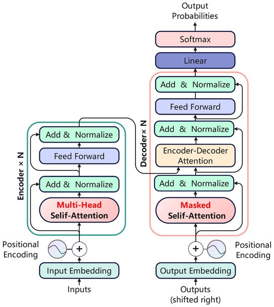
Figure 1. Transformer model architecture.

2.2. Multi-Head Attention

The model’s core architecture consists of a multi-head self-attention mechanism and a feed-forward neural network, as depicted in Figure 2. The multi-head attention mechanism operates by projecting input vectors into various subspaces, where multiple sets of scaled dot-product attention are computed in parallel to capture dependencies across different positions. Within each head, the Query (Q), Key (K), and Value (V) vectors are calculated independently.

$$q_i=W_q{x}_i\begin{array}{cc},& \end{array}i=1,2,\dots ,n$$

(1)

$$Q=\left[\begin{array}{cccc}{q}_1& q_2& \dots & q_n\end{array}\right]$$

(2)

$$k_i=W_k{x}_i\begin{array}{cc},& \end{array}i=1,2,\dots ,n$$

(3)

$$K=\left[\begin{array}{cccc}{k}_1& k_2& \dots & k_n\end{array}\right]$$

(4)

$$v_i=W_v{x}_i\begin{array}{cc},& \end{array}i=1,2,\dots ,n$$

(5)

$$V=\left[\begin{array}{cccc}{v}_1& v_2& \dots & v_n\end{array}\right]$$

(6)

where W_q, W_k and W_v are the weight matrices corresponding to the input, and Q, K, and V are the matrices formed by these weights. The similarity or matching degree between Q and each K is measured by calculating the dot product between the Q matrix and the K matrix. To prevent the Softmax function from entering a saturation region when calculating attention weights, a scaling factor, $\sqrt{d_k}$, is introduced. Dividing the dot product result by this scaling factor ensures that the input to the Softmax function remains within a reasonable range.

$$s(q_i,k_i)={\displaystyle \frac{q_i\bullet K}{\sqrt{d_k}}}$$

(7)

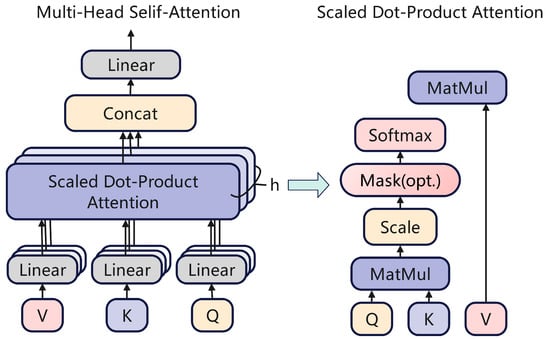
Figure 2. Multi-head attention mechanism.

The scaled dot-product is passed through a Softmax function to derive the attention weights for each Key with respect to the Query. Subsequently, the final output is computed as a weighted sum of the Value matrix, where the weights are the attention scores just calculated.

$$Attention(Q,K,V)=softmax({\displaystyle \frac{Q{K}^T}{\sqrt{d_k}}})V$$

(8)

The mechanism operates by projecting the input into multiple subspaces, yielding h distinct sets of Query (Q), Key (K), and Value (V) vectors. Each set independently computes an attention output. These h outputs are then concatenated and subsequently projected back to the original dimensionality via a final linear transformation.

$$Multihead(Q,K,V)=Concat(hea{d}_1,\dots ,hea{d}_h)W^0$$

(9)

$$hea{d}_i=Attention(Q{W}_i^Q,K{W}_i^V,V{W}_i^V)$$

(10)

The multi-head attention mechanism enables the model to dynamically attend to salient information across different sequence positions, thereby effectively capturing long-range dependencies. This provides a robust feature extraction capability for the subsequent time-series prediction task.

3. Experimental Setup and Model

3.1. Specimen Fabrication and Curing

The concrete specimens were designed for a C45 compressive strength and were cast using Ordinary Portland Cement (P·O 42.5, Qinghai New Type Construction Materials Industry and Trade Co., Ltd., Xining, China). The detailed mix proportions are presented in Table 1. Three specimens, each measuring 150 mm × 150 mm × 515 mm, were fabricated in this study. Prestressing force was applied via the post-tensioning method. Following 24 h of initial curing, the specimens were demolded and subsequently transferred to a standard curing room (20 °C, 95% RH) until the age of 28 days.

Table 1. Component preparation mix proportion.

Material	Water	Cement	Sand	Gravel
Dosage/(kg·m−3)	180	367	639	1213
Concrete mix proportion	0.49	1	1.74	3.3

To achieve axial loading in the concrete, a 20 mm diameter PVC duct was centrally embedded within each specimen. A 1860 MPa grade, 15.2 mm nominal diameter prestressing strand was installed in a straight profile. The strand was tensioned from a single end (single-end tensioning), with the arrangement detailed in Figure 3. The prestressing force was monitored indirectly via a pressure sensor positioned between the anchorage and the bearing plate. A tensioning force of 90 kN was applied using a miniature hydraulic jack. Slight variations in the initial prestress among the three specimens were observed, caused by an anchorage set-back of approximately 1 mm post-tensioning. The pressure sensor measured the effective anchorage force at the tensioning end, thereby implicitly accounting for the friction losses along the PVC duct during the initial tensioning phase. The values presented in Table 2 represent the effective initial prestress acting on the concrete specimens at the start of the freeze–thaw cycles.

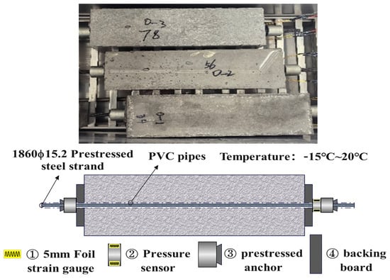
Figure 3. Testing arrangement.

Table 2. Initial prestressing of components.

Component Number	Number of Freeze–Thaw Cycles	Initial Prestress (MPa)
F-a	50	245.86
F-b	50	273.49
F-c	50	240.88

3.2. Freeze–Thaw Cycling Experiment

The freeze–thaw tests were conducted using a TDS-300 automatic freeze–thaw testing machine (Suzhou Donghua Test Instrument Co., Ltd., Suzhou, China), adopting the “air-freezing and water-thawing” method in strict accordance with the Chinese standard GB/T 50082-2024 [29]. Each cycle comprised 4 h of freezing and 4 h of thawing. To ensure uniform temperature distribution across the 150 mm cross-section, the testing machine utilized a forced air circulation system to maintain a homogeneous ambient temperature field. The 4-h duration for each phase was determined through pre-tests to ensure that the core temperature of the specimens reached the target range (−10 °C during freezing and +20 °C during thawing), effectively addressing the thermal gradient issue. Three specimens underwent 50 cycles, amounting to a total test time of 400 h (about 17 days). Throughout the experiment, variations in prestress were monitored at a sampling frequency of 0.1 Hz using a DH5922D data acquisition instrument (Donghua Testing Technology Co., Ltd., Jingjiang, China) integrated with the DHDAS dynamic signal acquisition and analysis system. The experimental arrangement is illustrated in Figure 4. The resulting time-series data, documenting the prestress evolution for each of the three specimens, formed the complete dataset used for subsequent model training and testing.

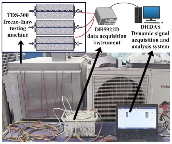
Figure 4. Test site layout.

3.3. Model Architecture and Training

The architecture of the prestress prediction model comprises an input layer, a positional encoding layer, a Transformer encoder, and an output layer. Initially, the input time-series data is projected into a high-dimensional feature space (model dimension: 128) via a linear layer. A positional encoding module then incorporates sequential order information into the sequence using sinusoidal functions, addressing the Transformer’s lack of inherent temporal awareness. The core of the model is a Transformer encoder, which is composed of 4 stacked blocks, each containing a multi-head self-attention mechanism (16 heads) and a feed-forward network. This architecture is designed to capture long-range dependencies within the time series. Ultimately, the output layer projects the encoder’s high-dimensional representation back to the target prediction dimension. The model employs a direct multi-step forecasting strategy. The final multi-step forecast is obtained by taking the last 50 time steps of the resulting output sequence. The selection of hyperparameters was based on a combination of empirical scaling rules derived from the foundational Transformer architecture [28] and preliminary trials on the validation set. Specifically, the model dimension (128) and number of heads (16) follow the standard architectural design principles of the Transformer, balancing computational efficiency with feature representation capability. The 4-layer encoder configuration was chosen to prevent overfitting, given the limited size of the training dataset. The stable convergence of the validation loss confirms that this configuration effectively captures the data patterns without overfitting, validating the rationality of the chosen parameters.

As illustrated in Figure 5, the prediction model utilizes the specimen’s prestress as both its input feature and target variable. All data was normalized with MinMaxScaler. It should be noted that MinMaxScaler is a linear transformation that preserves the relative amplitude of signal features; hence, anomalous spikes in the original data were retained in the normalized dataset. The dataset from specimen F-a was designated for training, while data from F-b and F-c were reserved exclusively for testing. The training set was further partitioned into an 80% training subset and a 20% validation subset.

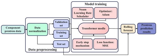
Figure 5. Model processing flow.

For model training, Mean Squared Error (MSE) was chosen as the loss function, with Adam as the optimizer. Given the Transformer model’s sensitivity to the learning rate, the Noam learning rate scheduler was implemented to facilitate stable and efficient convergence. This scheduler begins with a linear “warm-up” phase, enabling rapid exploration of the parameter space, followed by a decay phase proportional to the inverse square root of the step number to ensure stable convergence to an optimal solution in later training stages. This dynamic adjustment is a standard practice in training Transformer models. To further enhance training stability and generalization, gradient clipping and an early stopping strategy were also incorporated.

For a comprehensive performance evaluation of the proposed Transformer model, a Long Short-Term Memory (LSTM) network was employed as a baseline. As a classic recurrent neural network, LSTM is widely adopted for time-series forecasting tasks. To ensure a fair comparison, the LSTM model was configured with a comparable parameter scale: a hidden dimension of 128 and 4 layers. Both models were trained and evaluated using identical datasets, training strategies (including early stopping and gradient clipping), and performance metrics.

4. Results

4.1. Transformer Model Training

Figure 6 illustrates the training metrics of the model. The training loss experienced a rapid decline during the initial phase (epochs 0–5), dropping sharply from approximately 0.06 to 0.01, an 83.3% reduction. Subsequently, it entered a slow convergence phase, stabilizing at a minimal level below 0.005 after 75 epochs. This fast-then-slow convergence pattern suggests the model’s effectiveness in capturing the primary data patterns. The validation loss followed a similar trend, also decreasing rapidly to around 0.01. Throughout the later stages of training, the validation loss was slightly higher than the training loss, but the discrepancy remained small (stabilizing at approximately 0.007). The consistent convergence of both losses demonstrates the model’s strong generalization ability and indicates no significant overfitting.

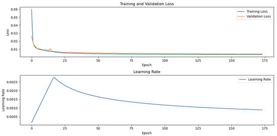
Figure 6. Model training metrics.

The learning rate curve exhibits the classic behavior of the Noam scheduler. During the initial warm-up phase (first ~16 epochs), the learning rate increased linearly to a peak of approximately 0.0028. It then transitioned into a gradual decay phase. This confirms that the Noam scheduler’s dynamic adjustment mechanism functioned as intended, with its pacing showing a strong synergy with the model’s convergence state. The learning rate strategy was well-matched to the loss function’s convergence characteristics, effectively balancing training speed with final precision.

Figure 7 illustrates the prediction results on the training data for specimen F-a. The plot shows the forecasting performance for the prestress time series beginning at data point 3932, with the blue solid line indicating the actual values and the red solid line representing the model’s predictions. A comparative analysis reveals that the model accurately captures the temporal trends of prestress, as the prediction curve aligns closely with the actual trajectory. Notably, the model maintains strong tracking performance even during periods of fluctuation in the prestress. Upon closer inspection of local details, a minor deviation between predicted and actual values is observable. The prediction error is markedly lower in stable intervals compared to intervals with abrupt changes, suggesting the model excels at predicting stationary time series. When abrupt changes occur, the model demonstrates rapid responsiveness and adjusts its prediction direction accordingly, showcasing good dynamic adaptability. While a slight lag is present in the prediction curve at these points of mutation, it still faithfully captures the overall trend of the data.

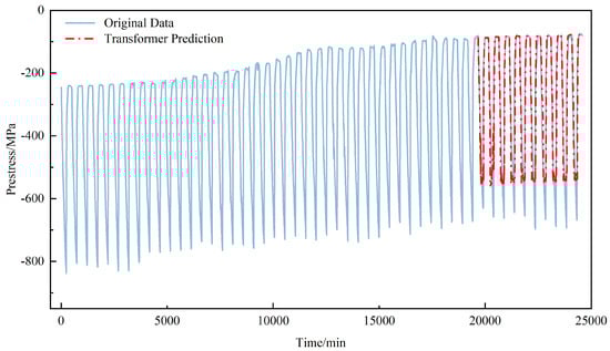
Figure 7. F-a component training prediction results.

4.2. Transformer Model Prediction

Figure 8 and Figure 9 illustrate the model’s prediction results on the F-b and F-c test sets. Both prestress datasets display distinct periodic fluctuations, which align with the freeze–thaw cycle process. The model’s predictions show a high degree of agreement with the actual data, accurately capturing these periodic patterns. However, dataset F-b contains a significant anomalous spike during the 38th cycle, where the prestress value abruptly increases by approximately 42 MPa above the expected periodic trend, forming a distinct outlier in the time series. While the model performs well on the regular periodic segments, it fails to accurately capture this abrupt anomaly. Instead, the prediction curve continued the established periodic pattern, missing the sudden jump in the actual data. This highlights the model’s limited capability in identifying atypical events. These findings demonstrate the model’s excellent performance on periodic data, achieving high-precision forecasts on the regular segments of both F-c and F-b. Under stable conditions, the predicted waveform closely matches the actual waveform, confirming the model’s predictive stability and reliability.

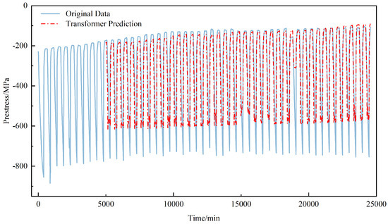
Figure 8. F-b Transformer model prediction results.

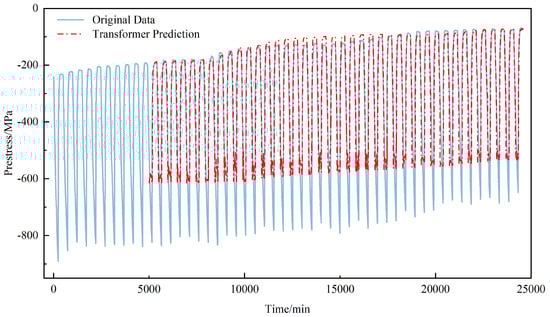
Figure 9. F-c Transformer model prediction results.

An analysis of the prediction results in Figure 7, Figure 8 and Figure 9 indicates a significant performance discrepancy between the thawing and freezing stages. While the model accurately predicts the phase and amplitude during thawing, its performance degrades considerably during freezing. To investigate this stage-dependent behavior, the freeze–thaw cycle was divided into distinct freezing and thawing phases, and prediction errors were computed for each on the F-c test set. As shown in Figure 10, the model’s accuracy in the thawing phase (R² = 0.8354, RMSE = 86.58 MPa) substantially surpasses that in the freezing phase (R² = 0.3315, RMSE = 110.84 MPa). This disparity is primarily attributed to the fixed sampling frequency of the data acquisition system. The relatively brief freezing plateau (~10 min), compared to the extensive thawing plateau (~175 min), provides a sparser dataset for the freezing phase. This data scarcity, combined with the rapid dynamics of the freezing process, impeded the model’s ability to learn the underlying patterns effectively. Conversely, the gradual thawing process yields a denser data profile at the same sampling frequency, enabling more precise modeling and prediction. Additionally, the fixed sampling frequency of 0.1 Hz, while capturing the gradual thawing process effectively, may have aliased or missed high-frequency stress waves generated during the rapid micro-crack formation and ice nucleation in the freezing phase, further contributing to the model’s limited performance in this stage.

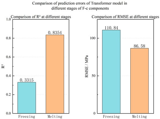
Figure 10. Comparison of prediction errors of Transformer model in different stages of F-c components.

4.3. Comparison Between Transformer and LSTM

To further substantiate the superiority of the proposed Transformer model, its performance was benchmarked against an LSTM. Figure 11 and Figure 12 illustrate the comparative prediction results on the F-b and F-c test sets, respectively. A visual inspection confirms that the Transformer model (blue solid line) exhibits a substantially higher fidelity to the true values (black solid line) compared to the LSTM model (red dotted line). The Transformer demonstrates precision in capturing the peaks of the prestress time series. The LSTM, by contrast, while roughly locating the peak positions, tends to overestimate their magnitudes. Although both models show deficiencies in predicting the troughs, the Transformer’s predictions are considerably closer to the true values. This discrepancy in the LSTM’s performance can be attributed to its limited capacity for modeling long-range dependencies, which results in excessive smoothing of the prediction curve and a consequent distortion of the waveform.

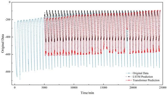
Figure 11. Comparison of F-b component Transformer model and LSTM prediction results.

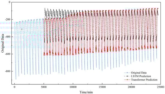
Figure 12. Comparison of F-c component Transformer model and LSTM prediction results.

To further quantify the performance of the proposed prestress prediction model against the LSTM, Table 3 presents a detailed comparison of key metrics—including Mean Squared Error (MSE), Root Mean Squared Error (RMSE), Mean Absolute Error (MAE), and the coefficient of determination (R²)—across three test sets. The results unequivocally demonstrate the superior performance of the Transformer model across all datasets. On the F-c test set, the Transformer achieved an R² of 0.8425, markedly higher than the LSTM’s 0.6754, signifying a superior capacity to explain data variance. Concurrently, its lower MSE, RMSE, and MAE values confirm higher prediction accuracy. On the F-b test set, despite the influence of anomalous data points on both models, the Transformer maintained a higher R² (0.7814 vs. 0.5702 for LSTM), highlighting its greater robustness in handling complex data patterns. In conclusion, the quantitative results in Table 3 are in strong agreement with the qualitative analysis from Figure 10 and Figure 11. The Transformer model, leveraging its powerful capability for capturing long-range dependencies, significantly outperforms the LSTM model in modeling the complex patterns of prestress time-series data, thereby validating its effectiveness and superiority for demanding engineering prediction applications. Although this study benchmarks the Transformer against LSTM, the advantages observed are structurally applicable to other conventional models like CNN-based approaches and support vector regression (SVR). CNN-based time series models have been shown to have limitations in capturing long-term dependencies and global context, particularly for long-interval forecasting scenarios, while SVR lacks an explicit mechanism for sequential dependency modeling. In contrast, LSTM represents a widely adopted sequential baseline designed to capture long-term temporal dependencies, making it a strong and sufficient reference for evaluating the Transformer’s ability to model complex temporal dynamics [30].

Table 3. Performance evaluation results.

Component Number	Model	Mean Square Error (MSE)	Root Mean Square Error (RMSE)	Mean Absolute Error (MAE)	Determination Coefficient (R2)
F-a	Transformer	6715.5667	81.9486	47.7438	0.8404
	LSTM	4562.7761	67.5483	50.2848	0.7769
F-b	Transformer	9167.6322	95.7478	61.7059	0.7814
	LSTM	21,934.6599	148.1035	106.4079	0.5702
F-c	Transformer	8039.8839	89.6654	57.4143	0.8425
	LSTM	13,611.0097	116.6662	78.5956	0.6754

5. Discussion

The evolution of prestress under freeze–thaw cycles represents a quintessential multi-scale process, where rapid stress fluctuations within a single cycle coexist with long-term cumulative degradation over numerous cycles. The Transformer’s self-attention mechanism is uniquely capable of concurrently attending to the inception and termination of a fluctuation cycle, thus comprehending the intra-cycle damage. Simultaneously, it can directly associate the state of the 1st cycle with that of the 50th, effectively capturing long-term degradation trends—a capability that is fundamentally challenging for LSTM due to the constraints of its recursive memory.

Despite the overall superior predictive performance of the proposed Transformer model, it failed to accurately capture the anomalous spike observed during the 38th cycle of specimen F-b (Figure 8), instead adhering to the established periodic pattern, with particularly poor predictions during the freezing phase of that cycle. This phenomenon exposes the intrinsic limitations of purely data-driven models. The Transformer model learns by internalizing statistical regularities from training data, predicated on the core assumption that future data will adhere to a distribution similar to historical data. When confronted with anomalous events absent from the training set that potentially contravene conventional physical evolutionary pathways, the model is inclined to treat them as statistical noise and smooth them over. This smoothing effect on anomalies suggests that the model optimizes for the dominant periodic pattern but lacks the physical constraints to identify irregular damage evolution. Physically, such an anomaly could signify the sudden coalescence of internal micro-cracks or the abrupt accumulation of localized damage within the concrete—an irreversible damage event. The model’s failure to identify this underscores its lack of explicit encoding for the fundamental constraints governing physical laws. Specifically, given the higher initial prestress in F-b (273.49 MPa), we hypothesize that it may have induced a higher stress concentration in the concrete matrix, potentially leading to sudden localized crushing or minor anchorage slip at a critical point, rather than solely gradual freeze–thaw degradation. Beyond this deficiency in discerning such anomalies, the model’s performance during normal freeze–thaw cycles is not impeccable, exhibiting significant stage dependency.

The performance disparity between the freezing and thawing stages (Figure 10) is especially stark, a discrepancy rooted in a mismatch between the data acquisition strategy and the dynamic characteristics of the physical process. While we have attributed this to the relative data sparsity during the freezing stage under a fixed sampling frequency, the implications of this finding are far more profound. It compellingly reveals the decisive influence of data quality on model performance and illuminates a clear path for optimization. A freeze–thaw cycle is a non-equilibrium thermodynamic process wherein the freezing stage involves the rapid nucleation and volumetric expansion of ice crystals, inducing drastic and transient stress changes (plateau ~10 min). This rapid volumetric expansion (approx. 9% volume increase) generates highly nonlinear internal bursting pressures within minutes. The model, trained primarily on data from the slower thawing phase, lacks sufficient examples of these rapid, high-magnitude stress fluctuations to learn the underlying pattern effectively. In contrast, the thawing stage is a relatively slow process of heat conduction and phase change (plateau ~175 min). Under a fixed sampling frequency, the gradual thawing process is captured with high density and detail, furnishing the model with ample learning samples, whereas the rapid freezing process is sparsely sampled, leading to a loss of critical dynamic information. This constitutes more than a mere technical deficiency in data acquisition; it reflects a fundamental misalignment between the current monitoring strategy and the critical phases of the physical process. Regarding the effect of noise or measurement uncertainty, the self-attention mechanism offers inherent robustness by focusing on high-saliency features and suppressing background noise. In this study, data normalization was applied during preprocessing to mitigate sensor bias. However, the distinct performance drop during the freezing phase suggests that the current sampling strategy is sensitive to rapid signal fluctuations, indicating a need for adaptive sampling or denoising strategies in future applications.

This performance disparity, a consequence of data quality, naturally prompts another pivotal question: how does the model generalize across different physical conditions when data quality is held constant? As presented in Table 3, the model’s R² value on the F-b test set (0.7814) is substantially lower than its performance on the F-c test set (0.8425). To investigate, we examined the initial prestress values for each specimen (Table 2). Notably, the initial prestress of F-b (273.49 MPa) was markedly higher than that of F-a (245.86 MPa) and F-c (240.88 MPa). We therefore posit that the initial prestress level governs the intrinsic modality of damage evolution. A higher initial stress implies that the concrete matrix was subjected to greater loads prior to the onset of freeze–thaw cycles, which could precipitate more accelerated and severe development of internal micro-cracks. This, in turn, renders the entire prestress loss process more nonlinear and stochastic. Such complex dynamics, induced by high-stress conditions, invariably elevate the prediction challenge for data-driven models. Furthermore, the heterogeneity of the concrete matrix—including variations in aggregate distribution and the presence of micro-voids—can alter local thermal conductivity and stress concentrations, rendering the prestress loss process more stochastic and challenging to predict with a purely data-driven model. We hypothesize that the higher initial stress level may induce more complex nonlinear damage patterns. While the model’s performance drop on F-b supports this view, strictly speaking, this remains a hypothesis requiring further mechanical validation. The dataset, although limited to three specimens, covers a range of initial prestress conditions (240.88 MPa to 273.49 MPa). The model’s successful prediction on F-c (with initial prestress similar to F-a) and reasonable performance on F-b (with higher initial prestress) suggest that the proposed framework possesses a certain degree of generalizability. However, the performance drop on F-b also highlights that specimen-specific characteristics significantly influence prediction accuracy. Future research aimed at developing more universal predictive models should therefore incorporate the initial prestress level as a crucial input feature, empowering the model to learn and adapt to damage evolution patterns across a spectrum of stress levels.

Regarding scalability, the Transformer model is computationally efficient during the inference phase, providing predictions in milliseconds, which is significantly faster than traditional Finite Element Method (FEM) simulations for long-term degradation prediction. The primary computational cost lies in offline training and periodic retraining. For real-world bridges with numerous sensors, adaptive sampling strategies could be employed to balance capturing rapid freezing dynamics and managing data storage costs. Furthermore, the current model is trained on data under static freeze–thaw conditions. Extending this framework to structures simultaneously subjected to dynamic traffic loads requires addressing complex multi-physics coupling effects, which represents a significant challenge for future research.

Finally, the benchmark comparison with LSTM offers a profound physical explanation for the Transformer’s structural superiority. As depicted in Figure 11 and Figure 12, the LSTM’s prediction curve is characterized by “phase lag and amplitude distortion.” Specifically, the LSTM’s predicted waveform consistently trails the measured data curve in time. More critically, its predicted extreme values during peaks and troughs often deviate from the true extremes, with its predictions at troughs being significantly higher than the actual values. This is a direct manifestation of its recursive computation and memory decay. Owing to the inherent latency and attenuation in information transfer across time steps, it cannot respond to rapid signal transitions with the requisite timeliness and precision. In stark contrast, the Transformer’s parallel self-attention mechanism empowers it to “simultaneously perceive” any two points across the entire sequence. It does not “remember” the past through sequential information passing but rather “understands” the global context by holistically computing correlation weights among all points in the sequence. When forecasting the next time step, the Transformer can concurrently “reference” all relevant patterns from the entire historical sequence, including the morphology of the preceding peak and the velocity of change in the current cycle. This global information integration faculty enables it to generate more timely and accurate predictions, thereby faithfully reproducing the dynamic characteristics of prestress evolution under freeze–thaw cycles. This serves as powerful evidence that for time-series prediction tasks characterized by clear physical periodicity and stringent phase accuracy requirements, the Transformer possesses a natural, structurally inherent advantage over LSTM that is simply incomparable.

6. Conclusions

This study proposes and validates a deep learning model based on the Transformer architecture to predict the dynamic evolution of prestress in concrete members under freeze–thaw cycles. This model provides a novel and more efficient technical approach for predicting prestress variations in prestressed concrete members within freeze–thaw environments. For bridge and infrastructure monitoring agencies, this model offers a promising tool for real-time condition assessment and proactive maintenance scheduling in cold regions, potentially reducing life-cycle costs and enhancing structural safety. Based on the experimental results and analysis, the main conclusions are drawn as follows:

(1)

The proposed Transformer model effectively captures the long-range dependencies and complex periodic patterns within the prestress time-series data, demonstrating high fidelity in tracking the dynamic evolution of prestress under freeze–thaw cycles.

(2)

The model’s performance is critically dependent on data quality and the physical conditions of the system. The model performs excellently during the gradual thawing phase but faces challenges during the rapid freezing phase due to data sparsity. Furthermore, the initial prestress level was identified as a key factor affecting the model’s generalization capability, as higher initial stress induces more complex nonlinear damage patterns.

(3)

Comparative experiments with the LSTM model further indicate that the Transformer model achieves comprehensive superiority across key performance metrics, including MSE, RMSE, MAE, and R². This advantage stems not only from algorithmic performance but is also rooted in its fundamental structural difference: the global attention mechanism of the Transformer is inherently more suitable for capturing the phase and amplitude of physically periodic signals, overcoming the inherent “phase lag and amplitude distortion” issues found in LSTM’s recursive memory.

Finally, while the proposed Transformer model demonstrates high prediction accuracy, it functions as a “black box” without explicit encoding of physical laws. A critical safety risk is the potential to smooth over anomalous but critical spikes in prestress, which could indicate impending failure. Consequently, in real-world structural health monitoring, this data-driven model should be deployed as a supplementary decision-support tool alongside physical sensor thresholds and expert judgment, rather than a standalone replacement. Its outputs must be interpreted within the bounds of established civil engineering safety codes and standards. To address these limitations and improve robustness, future work will focus on two aspects: first, conducting additional experimental campaigns with a wider variety of specimen characteristics to further validate the universality of the proposed approach. Second, exploring hybrid physics-informed or feature-augmented learning frameworks to integrate physical laws into the prediction process, thereby enhancing the model’s interpretability and its capability to identify critical damage states under complex environments.

References

- Li, X.Y.; Qin, L.H.; Guo, L.N.; Li, Y. Research on the Mechanical Properties of Concrete under Low Temperatures. Materials 2024, 17, 1882. [Google Scholar] [CrossRef]
- Lin, H.W.; Han, Y.F.; Liang, S.M.; Gong, F.Y.; Han, S.; Shi, C.W.; Feng, P. Effects of low temperatures and cryogenic freeze–thaw cycles on concrete mechanical properties: A literature review. Constr. Build. Mater. 2022, 345, 128287. [Google Scholar] [CrossRef]
- Xie, J.; Zhao, X.Q.; Yan, J.B. Experimental and numerical studies on bonded prestressed concrete beams at low temperatures. Constr. Build. Mater. 2018, 188, 101–118. [Google Scholar] [CrossRef]
- Omran, H.Y.; El-Hacha, R. Effects of Sustained Load and Freeze–Thaw Exposure on RC Beams Strengthened with Prestressed NSM-CFRP Strips. Adv. Struct. Eng. 2014, 17, 1801–1816. [Google Scholar] [CrossRef]
- Saiedi, R.; Green, M.F.; Fam, A. Behavior of CFRP-Prestressed Concrete Beams under Sustained Load at Low Temperature. J. Cold Reg. Eng. 2013, 27, 1–15. [Google Scholar] [CrossRef]
- Duo, Z.Y.; Gui, L.R.; Yu, C.; Kai, F. Experimental Study of Pre-Stressed Concrete Beams with Fatigue Subjoining Freezing-Thawing Circle. Adv. Mater. Res. 2011, 368–373, 2346–2350. [Google Scholar] [CrossRef]
- Davoodnabi, S.M.; Mirhosseini, S.M.; Shariati, M. Analyzing shear strength of steel-concrete composite beam with angle connectors at elevated temperature using finite element method. Steel Compos. Struct. 2021, 40, 853–868. [Google Scholar] [CrossRef]
- Shariati, M.; Raeispour, M.; Naghipour, M.; Kamyab, H.; Toghroli, A. Flexural behavior analysis of double honeycomb steel composite encased concrete beams: An integrated experimental and finite element study. Case Stud. Constr. Mater. 2024, 20, e03299. [Google Scholar] [CrossRef]
- Zhang, H.; Xia, J.F.; Zhou, J.T.; Liao, L.; Xiao, Y.J.; Tong, K.; Zhang, S.H. Prestress monitoring for prestress tendons based on the resonance-enhanced magnetoelastic method considering the construction process. Struct. Health Monit. 2024, 23, 958–970. [Google Scholar] [CrossRef]
- Zhi, C.S.; Gang, W.; Tuo, X.; Feng, D.C. Prestressing force monitoring method for a box girder through distributed long-gauge FBG sensors. Smart Mater. Struct. 2018, 27, 15015. [Google Scholar] [CrossRef]
- Wang, B.; Huo, L.S.; Chen, D.D.; Li, W.J.; Song, G.B. Impedance-Based Pre-Stress Monitoring of Rock Bolts Using a Piezoceramic-Based Smart Washer—A Feasibility Study. Sensors 2017, 17, 250. [Google Scholar] [CrossRef]
- Huynh, T.; Kim, J. FOS-Based Prestress Force Monitoring and Temperature Effect Estimation in Unbonded Tendons of PSC Girders. J. Aerosp. Eng. 2016, 30, B4016005. [Google Scholar] [CrossRef]
- Cao, D.F.; Qin, X.C.; Meng, S.P.; Tu, Y.M.; Elfgren, L.; Sabourova, N.; Grip, N.; Ohlsson, U.; Blanksvärd, T. Evaluation of prestress losses in prestressed concrete specimens subjected to freeze–thaw cycles. Struct. Infrastruct. Eng. 2016, 12, 159–170. [Google Scholar] [CrossRef]
- Wang, L.; Zhang, L.Y.; Di, M.; Wu, X.G. A PZT-Based Smart Anchor Washer for Monitoring Prestressing Force Based on the Wavelet Packet Analysis Method. Appl. Sci. 2024, 14, 641. [Google Scholar] [CrossRef]
- Wang, Z.W.; Lu, X.F.; Zhang, W.M.; Fragkoulis, V.C.; Zhang, Y.F.; Beer, M. Deep learning-based prediction of wind-induced lateral displacement response of suspension bridge decks for structural health monitoring. J. Wind Eng. Ind. Aerodyn. 2024, 247, 105679. [Google Scholar] [CrossRef]
- Xu, D.H.; Xu, X.; Michael, C.F.; Caballero, A. Concrete and steel bridge Structural Health Monitoring—Insight into choices for machine learning applications. Constr. Build. Mater. 2023, 402, 132596. [Google Scholar] [CrossRef]
- Calò, M.; Ruggieri, S.; Buitrago, M.; Nettis, A.; Adam, J.M.; Uva, G. An ML-based framework for predicting prestressing force reduction in reinforced concrete box-girder bridges with unbonded tendons. Eng. Struct. 2025, 325, 119400. [Google Scholar] [CrossRef]
- Nguyen, T.T.; Thi, T.V.P.; Ho, D.D.; Ananta, M.S.P.; Huynh, T.C. Deep learning-based autonomous damage-sensitive feature extraction for impedance-based prestress monitoring. Eng. Struct. 2022, 259, 114172. [Google Scholar] [CrossRef]
- Nguyen, T.T.; Hoang, N.; Nguyen, T.H.; Huynh, T.C. Analytical impedance model for piezoelectric-based smart Strand and its feasibility for prestress force prediction. Struct. Control Health Monit. 2022, 29, e3061. [Google Scholar] [CrossRef]
- Rizvi, S.H.M.; Abbas, M.; Zaidi, S.S.H.; Tayyab, M.; Malik, A. LSTM-Based Autoencoder with Maximal Overlap Discrete Wavelet Transforms Using Lamb Wave for Anomaly Detection in Composites. Appl. Sci. 2024, 14, 2925. [Google Scholar] [CrossRef]
- Min, S.; Lee, Y.; Byun, Y.H.; Jong, K.Y.; Kim, S. Merged LSTM-based pattern recognition of structural behavior of cable-supported bridges. Eng. Appl. Artif. Intell. 2023, 125, 106774. [Google Scholar] [CrossRef]
- Fathnejat, H.; Ahmadi-Nedushan, B.; Hosseininejad, S.; Noori, M.; Altabey, W.A. A data-driven structural damage identification approach using deep convolutional-attention-recurrent neural architecture under temperature variations. Eng. Struct. 2023, 276, 115311. [Google Scholar] [CrossRef]
- Jbene, M.; Chehri, A.; Saadane, R.; Tigani, S.; Jeon, G. From RNNs to Transformers and Beyond: A Deep Dive into Intent Detection in Goal-oriented Conversational Agents. Cogn. Comput. 2025, 17, 116. [Google Scholar] [CrossRef]
- Mousavi, V.; Rashidi, M.; Ghazimoghadam, S.; Mohammadi, M.; Samali, B.; Devitt, J. Transformer-based time-series GAN for data augmentation in bridge digital twins. Autom. Constr. 2025, 175, 106208. [Google Scholar] [CrossRef]
- Li, Z.Q.; Li, D.S.; Sun, T.S. A Transformer-Based Bridge Structural Response Prediction Framework. Sensors 2022, 22, 3100. [Google Scholar] [CrossRef]
- Rahmani, M.C.; Khatir, A.; Azad, M.M.; Kim, H.S.; Firouzi, N.; Kumar, R.; Khatir, S.; Cuong, L.T. Mechanics-based deep learning framework for predicting deflection of functionally graded composite plates using an enhanced whale optimization algorithm. Math. Mech. Solids 2026, 1, 10812865251398866. [Google Scholar] [CrossRef]
- He, Z.J.; Huang, T.L.; Chen, B. Physics-informed graph transformer network for predicting cable-stayed bridge structural deflection response. Adv. Eng. Inform. 2026, 69, 103897. [Google Scholar] [CrossRef]
- Vaswani, A.; Shazeer, N.; Parmar, N.; Uszkoreit, J.; Jones, L.; Gomez, A.N.; Kaiser, L.; Polosukhin, I. Attention is all you need. Adv. Neural Inf. Process. Syst. 2017, 30, 5998–6008. [Google Scholar] [CrossRef]
- GB/T 50082-2024; Standard for Test Methods of Long-Term Performance and Durability of Concrete. China Architecture & Building Press: Beijing, China, 2024.
- Liu, X.; Wang, W. Deep Time Series Forecasting Models: A Comprehensive Survey. Mathematics 2024, 12, 1504. [Google Scholar] [CrossRef]
Disclaimer/Publisher’s Note: The statements, opinions and data contained in all publications are solely those of the individual author(s) and contributor(s) and not of MDPI and/or the editor(s). MDPI and/or the editor(s) disclaim responsibility for any injury to people or property resulting from any ideas, methods, instructions or products referred to in the content. |
© 2026 by the authors. Licensee MDPI, Basel, Switzerland. This article is an open access article distributed under the terms and conditions of the Creative Commons Attribution (CC BY) license.